In this post we build a complete diffusion model from scratch — training a UNet on a custom dataset, implementing the full DDPM pipeline, and understanding the math that makes iterative denoising work. We cover noise schedules, the reparameterization trick, FID evaluation, and three diffusion objectives (ε, x₀, v). By the end you’ll have generated novel images from pure Gaussian noise, and understand why diffusion models overtook GANs as the dominant paradigm for image generation. So let’s begin!

Tutorial Overview:

1. The Wow Moment — Generating Images from Pure Noise
2. Under the Hood — Step-by-Step Sampling
3. Training Data — Loading the Dataset
4. The Forward Process — Adding Noise
5. The UNet — Architecture for Denoising
6. Training Loop — Teaching the Model to Denoise
7. Sampling — Generating New Images
8. Evaluation — FID Score
9. Noise Schedules In Depth
10. Effect of Resolution and Input Scaling
11. UNets In Depth
12. Diffusion Objectives — ε vs x₀ vs v
13. Alternative Architectures
14. Summary

1. The Wow Moment — Generating Images from Pure Noise

In our previous post we traced how the Transformer crossed over into computer vision through ViT  – patch embeddings, self-attention over spatial tokens, positional encodings adapted for image grids. That architectural flexibility is exactly what powers modern diffusion models. But before we get to the transformer variants at the frontier, we need to build the foundation: the DDPM pipeline, the UNet backbone, and the training and sampling mechanics. That is what this post covers.

GANs dominated image generation from 2014 onward. They produced stunning results — but were notoriously difficult to train. Mode collapse, unstable gradients, the constant adversarial game between generator and discriminator. We covered all of that in our GAN series and catalogued the tricks needed to stabilize them. By late 2020, a different paradigm had quietly surpassed GANs in image quality: diffusion models. By 2022, DALL·E 2 and Stable Diffusion made them mainstream.

The key insight is deceptively simple. Unlike VAEs or GANs — which must get everything right in a single forward pass — diffusion models iterate. They start from pure random noise and ask one small question at each step: what noise was added here? Subtract it. Ask again. After a thousand steps, you have an image.

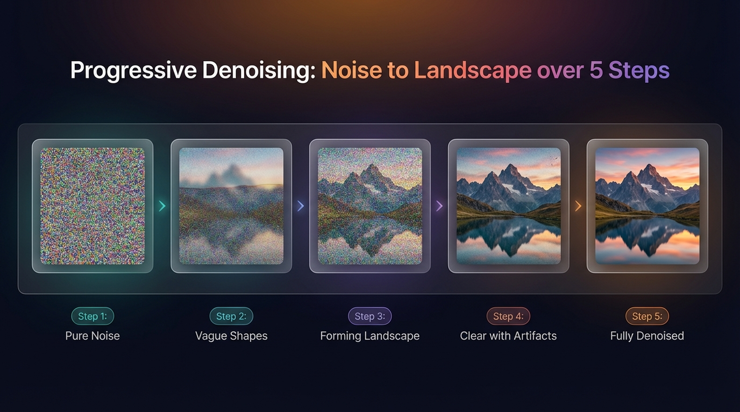
Before diving into how this works, let’s see it. Five lines of code, pure noise in, landscape out:

# !pip install diffusers torch accelerate
from diffusers import DDPMPipeline
import torch

device = torch.device("cuda" if torch.cuda.is_available() else "cpu")

image_pipe = DDPMPipeline.from_pretrained("google/ddpm-ema-church-256")
image_pipe.to(device)

image = image_pipe(num_inference_steps=1000).images[0]
image  # Display in Colab

Progressive denoising: Pure Noise → Vague Shapes → Forming Landscape → Clear with Artifacts → Fully Denoised. No single step produces a correct image — coherence emerges gradually across all 1000 steps.

Final output from the pretrained landscape model. This image did not exist in training data — synthesized entirely from pure Gaussian noise.

What you see above is the defining characteristic: each step corrects a small portion of the accumulated error, rather than betting everything on a single perfect generation. This iterative refinement is what GANs never had.

2. Under the Hood — Step-by-Step Sampling

The pipeline hides the mechanics. Let’s open it. This is the reverse process — going from noise back to image. At each step the model is shown the current noisy sample \(x_t\) and told the timestep. It predicts the noise component \(\varepsilon\) that was added. The scheduler then computes \(x_{t-1}\) — a slightly less noisy version. We do not jump straight to the predicted clean image \(\hat{x}_0\): we nudge \(x_t\) just a small step toward it, then re-predict from the new position. This conservative stepping is what makes diffusion stable — and slow.

sample = torch.randn(4, 3, 256, 256).to(device)
image_pipe.scheduler.set_timesteps(num_inference_steps=40)

steps_to_show = [0, 10, 20, 39]
fig, axes = plt.subplots(len(steps_to_show), 2, figsize=(8, 12))

for i, t in enumerate(image_pipe.scheduler.timesteps):
    with torch.inference_mode():
        noise_pred = image_pipe.unet(sample, t)["sample"]

    # Derive predicted clean image x0 from noise prediction (visualization only)
    # x0 = (x_t - sqrt(1 - alpha_bar) * eps) / sqrt(alpha_bar)
    alpha_t = image_pipe.scheduler.alphas_cumprod[t]
    predicted_x0 = (sample - (1 - alpha_t).sqrt() * noise_pred) / alpha_t.sqrt()

    # Scheduler computes x_{t-1}: small step toward predicted_x0, not a jump
    scheduler_output = image_pipe.scheduler.step(noise_pred, t, sample)
    sample = scheduler_output.prev_sample  # This is x_{t-1}

    if i in steps_to_show:
        row = steps_to_show.index(i)
        img_noisy = (sample[0].cpu().permute(1,2,0)*0.5+0.5).clip(0,1)
        axes[row, 0].imshow(img_noisy)
        axes[row, 0].set_title(f"Step {i}: Current x")
        axes[row, 0].axis("off")
        img_pred = (predicted_x0[0].cpu().permute(1,2,0)*0.5+0.5).clip(0,1)
        axes[row, 1].imshow(img_pred)
        axes[row, 1].set_title(f"Step {i}: Predicted x0")
        axes[row, 1].axis("off")

plt.tight_layout()
plt.show()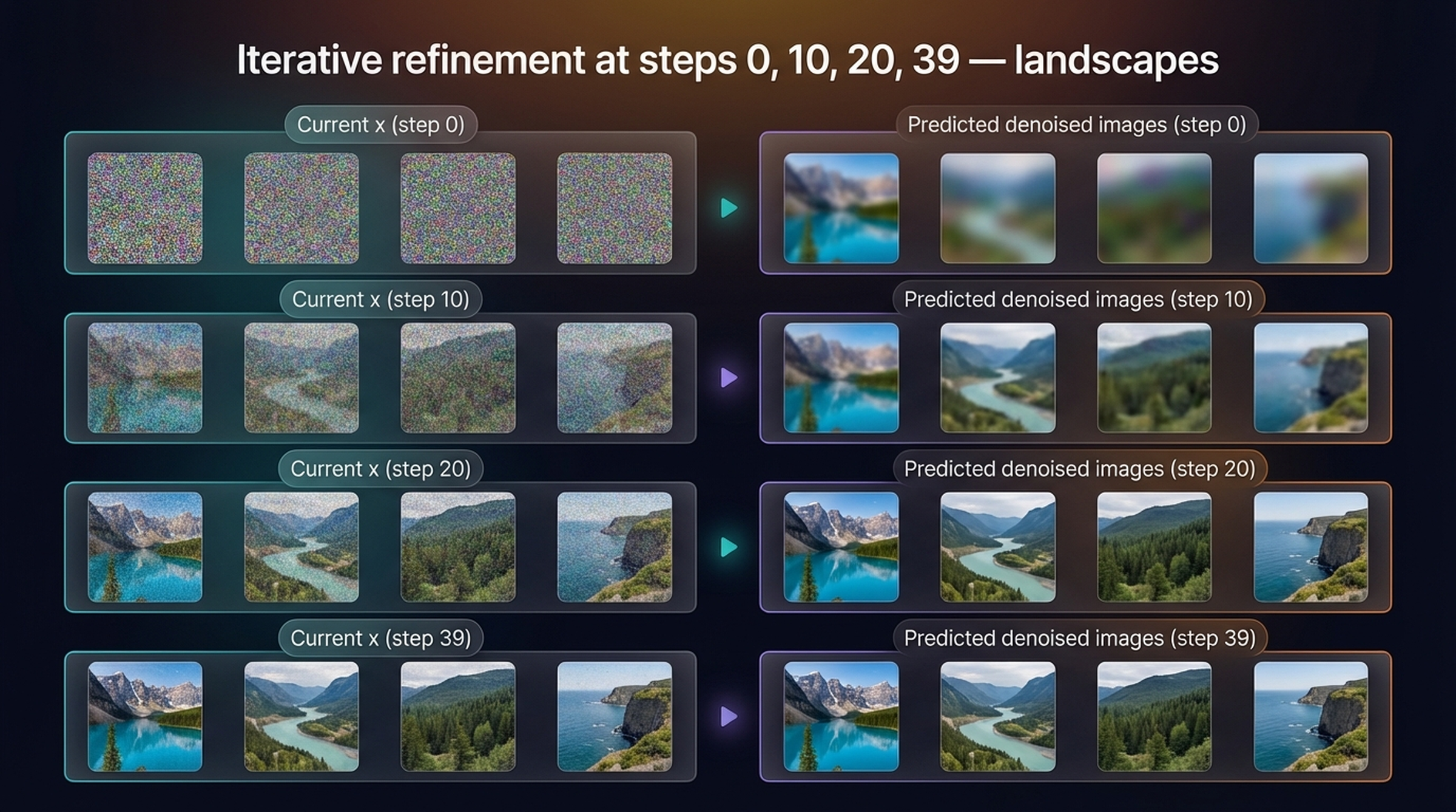

Left: \(x_t\) — the actual sample being denoised step by step. Right: \(\hat{x}_0\) — the model’s current best guess at the final clean image. At step 0 the guess is noisy and vague. By step 10 coarse structure appears. By step 39 both converge to a sharp, coherent image.

3. Training Data — Loading the Dataset

Now we train from scratch. We use the Smithsonian butterflies dataset [2] — 1000 images, small enough to train in Colab in under an hour on a free T4 GPU.

Training data diversity is critical. The model must learn the full distribution — texture, shape, color, background — to generate convincing novel samples.

from torchvision import transforms
from datasets import load_dataset
from torch.utils.data import DataLoader

dataset = load_dataset("huggan/smithsonian_butterflies_subset", split="train")

IMAGE_SIZE = 64

preprocess = transforms.Compose([
    transforms.Resize((IMAGE_SIZE, IMAGE_SIZE)),
    transforms.RandomHorizontalFlip(),
    transforms.ToTensor(),
    transforms.Normalize([0.5], [0.5]),    # Map [0,1] to [-1,1]
])

def transform(examples):
    examples = [preprocess(image) for image in examples["image"]]
    return {"images": examples}

dataset.set_transform(transform)
train_dataloader = DataLoader(dataset, batch_size=16, shuffle=True)

batch = next(iter(train_dataloader))
print(f"Batch shape: {batch['images'].shape}")  # (16, 3, 64, 64)

Normalization to \([-1, 1]\) is important: it centers pixel values around zero, matching the zero-mean Gaussian noise we will be adding. Mixing images in \([0, 1]\) with noise sampled from \(\mathcal{N}(0, I)\) would skew the signal-to-noise ratio throughout training.

4. The Forward Process — Adding Noise

Diffusion models are trained by learning to undo a destruction process. The forward process systematically corrupts clean images by adding Gaussian noise across 1000 timesteps until the image is indistinguishable from pure noise.

The key formula — the reparameterization trick — lets us jump to any noise level in a single step without iterating through all previous ones:

$$x_t = \bar{\alpha}_t^{1/2} \cdot x_0 + (1 – \bar{\alpha}_t)^{1/2} \cdot \varepsilon, \quad \varepsilon \sim N(0, I)$$

Where does this come from? It is not an assumption — it is the closed-form solution of a recurrence. Starting from \(x_t = \sqrt{\alpha_t} \cdot x_{t-1} + \sqrt{1-\alpha_t} \cdot z_t\) and expanding recursively, the signal component becomes a product of \(\sqrt{\alpha}\) terms while the noise becomes a weighted sum of independent Gaussians. A weighted sum of Gaussians is still Gaussian, so the entire chain collapses to a single noise term. This is why we can sample any timestep directly.

Here \(\bar{\alpha}_t = \prod_{s=1}^{t}(1 – \beta_s)\) is the cumulative product of noise coefficients. At \(t=0\): \(\bar{\alpha}_0 \approx 1\), so \(x_t \approx x_0\) (clean image). At \(t=1000\): \(\bar{\alpha}_{1000} \approx 0\), so \(x_t \approx \varepsilon\) (pure noise).

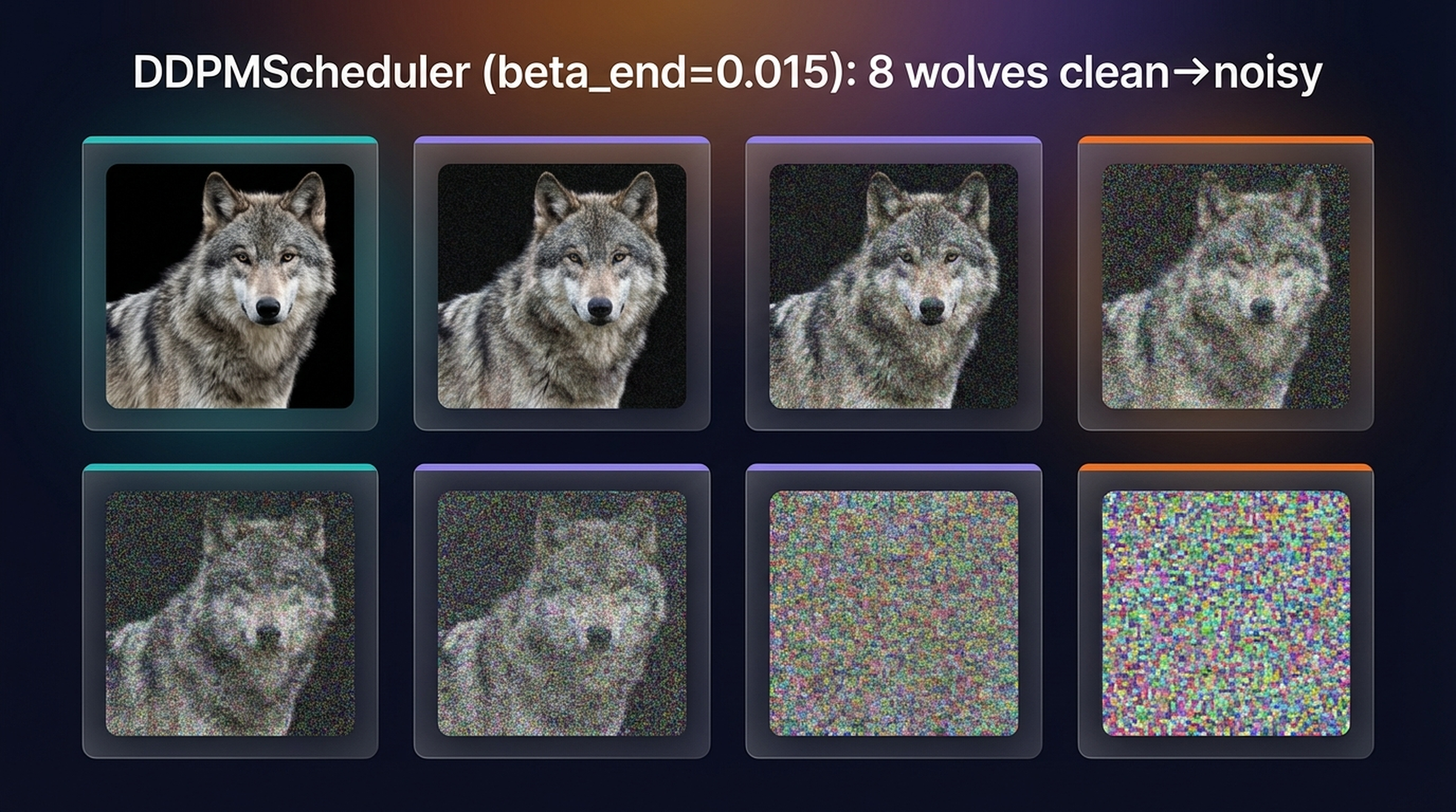
from diffusers import DDPMScheduler

noise_scheduler = DDPMScheduler(
    num_train_timesteps=1000,
    beta_start=0.001,
    beta_end=0.02
)

x = batch["images"][:1].to(device)
noise = torch.randn_like(x)
timesteps = torch.linspace(0, 999, 8).long()

fig, axes = plt.subplots(1, 8, figsize=(16, 2.5))
labels = ["Clean", "Mild", "Moderate", "Significant", "Heavy", "Extreme", "Near Pure", "Pure Noise"]

for i, t in enumerate(timesteps):
    noised_x = noise_scheduler.add_noise(x, noise, t.unsqueeze(0))
    img = (noised_x[0].cpu().permute(1, 2, 0) * 0.5 + 0.5).clip(0, 1)
    axes[i].imshow(img)
    axes[i].set_title(f"t={t.item():.0f}\n{labels[i]}", fontsize=8)
    axes[i].axis("off")

plt.tight_layout()
plt.show()

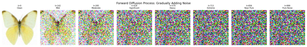
Forward diffusion on a butterfly from the training set. By \(t=570\) the image is unrecognizable. At \(t=999\) it is pure noise — identical in distribution to the random tensor we start from during sampling.

5. The UNet — Architecture for Denoising

We need a model that takes a noisy image plus a timestep and outputs the predicted noise — with the same spatial dimensions as the input. This is exactly the job of a UNet, originally invented for medical image segmentation in 2015.

The UNet has three structural properties that make it ideal here. The encoder-decoder structure compresses spatial information to a low-resolution bottleneck then expands it back. Skip connections between encoder and decoder layers pass fine-grained spatial detail directly across — critical for preserving sharp image features. And it naturally handles the same-size input/output constraint. Modern diffusion UNets add attention blocks at lower-resolution layers and residual connections throughout.

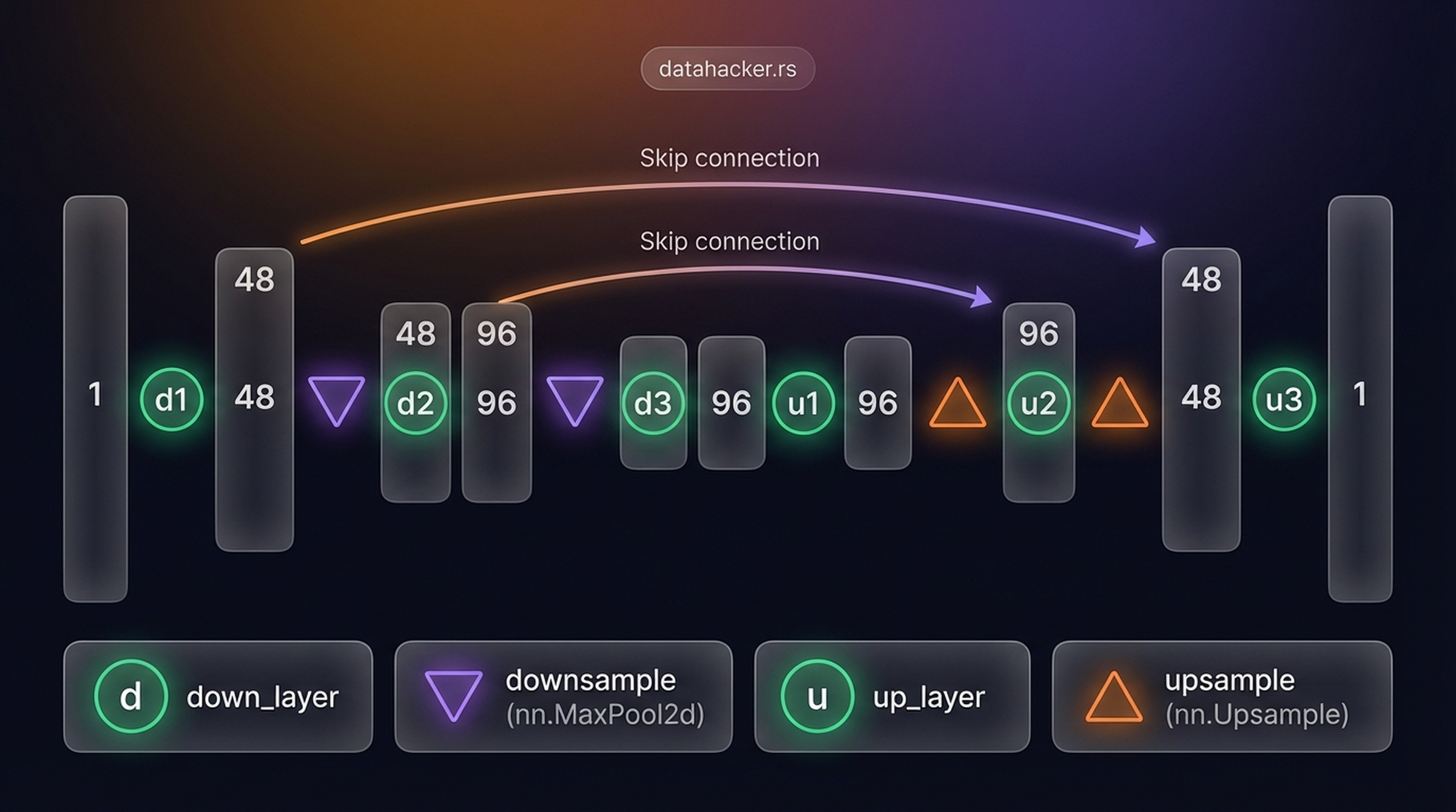
UNet architecture. The encoder halves spatial resolution while doubling channels. The decoder restores resolution. Skip connections pass encoder features directly to the corresponding decoder layer.

from diffusers import UNet2DModel

model = UNet2DModel(
    in_channels=3,
    out_channels=3,
    sample_size=IMAGE_SIZE,
    block_out_channels=(64, 128, 256, 512),
    down_block_types=(
        "DownBlock2D",
        "DownBlock2D",
        "AttnDownBlock2D",
        "AttnDownBlock2D",
    ),
    up_block_types=(
        "AttnUpBlock2D",
        "AttnUpBlock2D",
        "UpBlock2D",
        "UpBlock2D",
    ),
)
model = model.to(device)

with torch.inference_mode():
    noisy_batch = torch.randn(4, 3, IMAGE_SIZE, IMAGE_SIZE).to(device)
    t = torch.zeros(4, dtype=torch.long, device=device)
    output = model(noisy_batch, t)
    print(f"Input shape:  {noisy_batch.shape}")       # (4, 3, 64, 64)
    print(f"Output shape: {output['sample'].shape}")  # (4, 3, 64, 64)
    print(f"Parameters: {sum(p.numel() for p in model.parameters()):,}")

6. Training Loop — Teaching the Model to Denoise

The training procedure follows five steps per iteration: load a batch of clean images → add a random amount of noise (different timestep per image) → feed noisy images and timesteps into the UNet → predict the noise → minimize MSE between prediction and actual noise. This is the epsilon objective.

import torch.nn.functional as F

num_epochs = 50
lr = 1e-4
optimizer = torch.optim.AdamW(model.parameters(), lr=lr)
losses = []

for epoch in range(num_epochs):
    epoch_losses = []
    for batch in train_dataloader:
        clean_images = batch["images"].to(device)

        noise = torch.randn(clean_images.shape).to(device)

        timesteps = torch.randint(
            0, noise_scheduler.config.num_train_timesteps,
            (clean_images.shape[0],), device=device
        ).long()

        noisy_images = noise_scheduler.add_noise(clean_images, noise, timesteps)

        noise_pred = model(noisy_images, timesteps, return_dict=False)[0]

        loss = F.mse_loss(noise_pred, noise)
        losses.append(loss.item())
        epoch_losses.append(loss.item())

        loss.backward()
        optimizer.step()
        optimizer.zero_grad()

    avg = sum(epoch_losses) / len(epoch_losses)
    if (epoch + 1) % 10 == 0 or epoch == 0:
        print(f"Epoch {epoch+1}/{num_epochs}, Loss: {avg:.4f}")

Why predict noise rather than the clean image directly? Because at every timestep the amount of noise present varies enormously. Predicting the noise is a well-conditioned problem across all timesteps — at every noise level there is exactly one correct noise vector to find. We revisit this question in Section 12 when we compare epsilon, x₀, and v-prediction objectives.

An important subtlety: training samples timesteps randomly — the model never sees the sequence t=999, 998, 997, … during training. It learns to denoise at each noise level independently. Only during inference are the steps chained together sequentially.

fig, (ax1, ax2) = plt.subplots(1, 2, figsize=(12, 4))

ax1.plot(losses)
ax1.set_title("Training Loss (all steps)")
ax1.set_xlabel("Step"); ax1.set_ylabel("MSE Loss")

ax2.plot(range(500, len(losses)), losses[500:])
ax2.set_title("Training Loss (from step 500)")
ax2.set_xlabel("Step")

plt.tight_layout()
plt.show()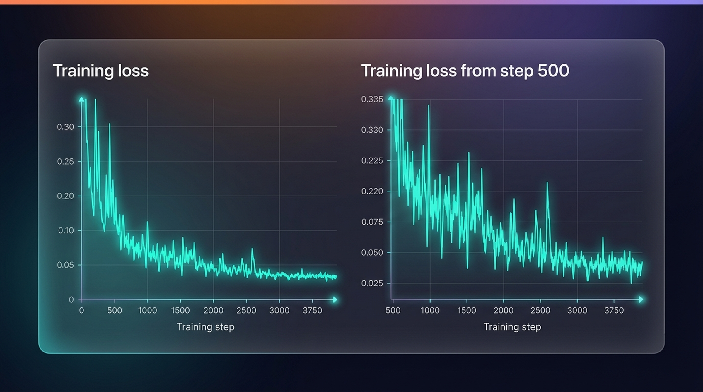

Training loss over 50 epochs. Sharp drop in the first 10 epochs, then slow convergence. The per-step variance is structural: each batch draws random timesteps, mixing easy near-clean denoising tasks with hard near-noise ones.

7. Sampling — Generating New Images

After training, generating new images is simply the reverse of the forward process. Start from pure Gaussian noise and iteratively apply the denoising model.

from diffusers import DDPMPipeline

# Method 1: DDPMPipeline (concise)
pipeline = DDPMPipeline(unet=model, scheduler=noise_scheduler)
pipeline.to(device)
images = pipeline(batch_size=4, num_inference_steps=1000).images
show_images(images, nrows=1, figsize=(12, 3))

# Method 2: Manual loop (see exactly what happens at each step)
noise_scheduler.set_timesteps(num_inference_steps=1000)
sample = torch.randn(4, 3, IMAGE_SIZE, IMAGE_SIZE).to(device)

for t in noise_scheduler.timesteps:
    with torch.inference_mode():
        noise_pred = model(sample, t)["sample"]
    sample = noise_scheduler.step(noise_pred, t, sample).prev_sample

generated = (sample.cpu() * 0.5 + 0.5).clip(0, 1)
show_images(generated, nrows=1, figsize=(12, 3))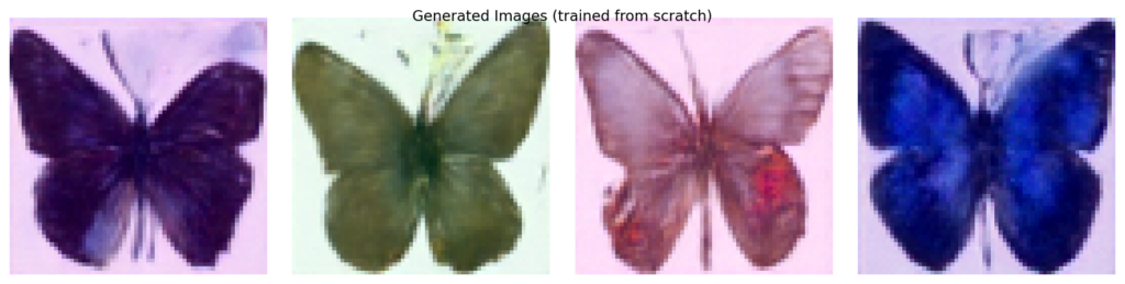

Four images generated from pure noise. The model has learned the statistical structure of the dataset — shape, color distribution, wing symmetry — well enough to synthesize coherent novel samples. None of these exist in the training set.

At 64×64 resolution, upscaled results show pixelation artifacts. This is a resolution limitation, not a model failure. At 256×256 (as in the pretrained landscape model) outputs are visually clean.

8. Evaluation — FID Score

How do we measure whether generated images look like real ones? Visual inspection is subjective and doesn’t scale. The standard metric is Fréchet Inception Distance (FID).

FID works by passing both real and generated images through a pretrained CNN (typically Inception v3) and extracting feature vectors from an intermediate layer. It fits a multivariate Gaussian to each feature set and computes the Fréchet distance between the two distributions. Lower FID = closer distributions = better quality.

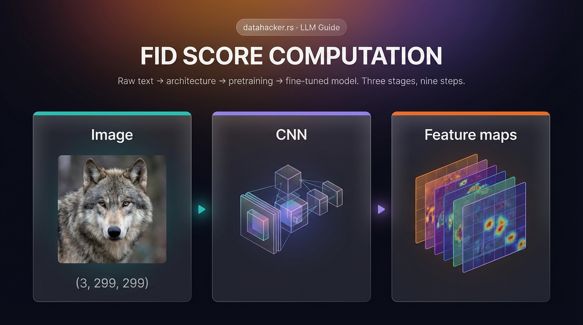
FID computation pipeline. Both real and generated images are passed through a pretrained CNN. Standard practice requires approximately 50,000 images for a reliable measurement.

Caveats: FID requires large sample sizes (50K minimum for stable measurements), is sensitive to image resolution and preprocessing format, and ImageNet-pretrained features may not generalize to unusual domains. Human preference studies remain the gold standard for judging generation quality in practice.

9. Noise Schedules In Depth

The noise schedule — how much noise gets added at each timestep — is a critical design choice.

9.1 Simple Scheduler

The simplest approach is linear interpolation between the clean image and pure noise:

def corrupt(x, noise, amount):
    """Linear interpolation: amount=0 means clean, amount=1 means pure noise."""
    amount = amount.view(-1, 1, 1, 1)
    return x * (1 - amount) + noise * amount


class SimpleScheduler:
    def __init__(self):
        self.num_train_timesteps = 1000

    def add_noise(self, x, noise, timesteps):
        amount = timesteps / self.num_train_timesteps
        return corrupt(x, noise, amount)

9.2 DDPM Scheduler

The DDPM paper uses a principled schedule based on the \(\beta_t\) parameters. Define \(\alpha_t = 1 – \beta_t\) and \(\bar{\alpha}_t = \prod_{s=1}^{t} \alpha_s\). The reparameterization formula \(x_t = \sqrt{\bar{\alpha}_t} \cdot x_0 + \sqrt{1-\bar{\alpha}_t} \cdot \varepsilon\) enables jumping to any timestep directly — critical for efficient training where we randomly sample timesteps per batch.

simple_sched = SimpleScheduler()
ddpm_sched = DDPMScheduler(beta_end=0.01)

x_demo = batch["images"][:1].to(device)
noise_demo = torch.randn_like(x_demo)
timesteps_demo = torch.linspace(0, 999, 8).long()

fig, axes = plt.subplots(2, 8, figsize=(16, 5))

for i in range(8):
    noised = simple_sched.add_noise(x_demo, noise_demo, timesteps_demo[i:i+1].to(device))
    img = (noised[0].cpu().permute(1,2,0)*0.5+0.5).clip(0,1)
    axes[0, i].imshow(img)
    axes[0, i].set_title(f"t={timesteps_demo[i].item():.0f}", fontsize=8)
    axes[0, i].axis("off")

    noised = ddpm_sched.add_noise(x_demo, noise_demo, timesteps_demo[i:i+1])
    img = (noised[0].cpu().permute(1,2,0)*0.5+0.5).clip(0,1)
    axes[1, i].imshow(img)
    axes[1, i].set_title(f"t={timesteps_demo[i].item():.0f}", fontsize=8)
    axes[1, i].axis("off")

axes[0, 0].set_ylabel("Simple", rotation=0, labelpad=45, fontsize=10)
axes[1, 0].set_ylabel("DDPM", rotation=0, labelpad=45, fontsize=10)
plt.suptitle("SimpleScheduler vs DDPMScheduler")
plt.tight_layout()
plt.show()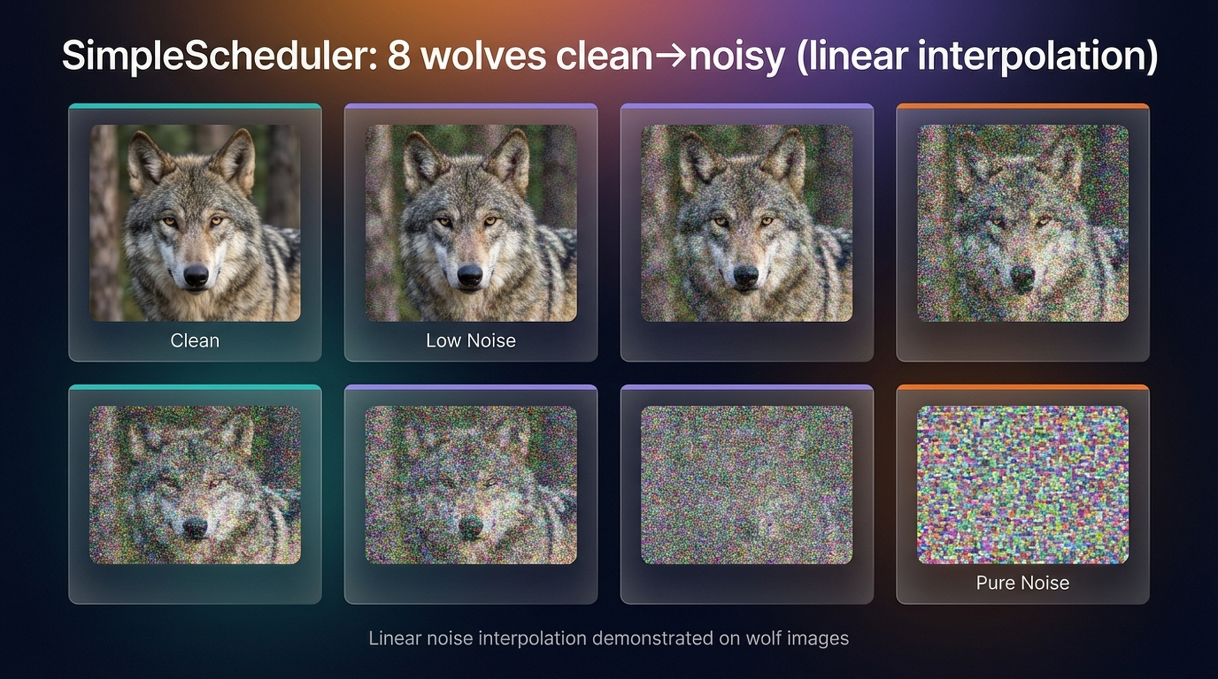

Top row: SimpleScheduler — linear interpolation. Bottom row: DDPMScheduler. Visually similar, but the DDPM schedule enables the reparameterization trick: any timestep is directly accessible in a single operation.

9.3 Schedule Shape — Linear vs Cosine

The shape of the \(\beta_t\) progression matters. A linear schedule adds noise at a constant rate. A cosine schedule adds noise slowly at first then accelerates — giving the model more training signal in the early regime where image structure is still visible.

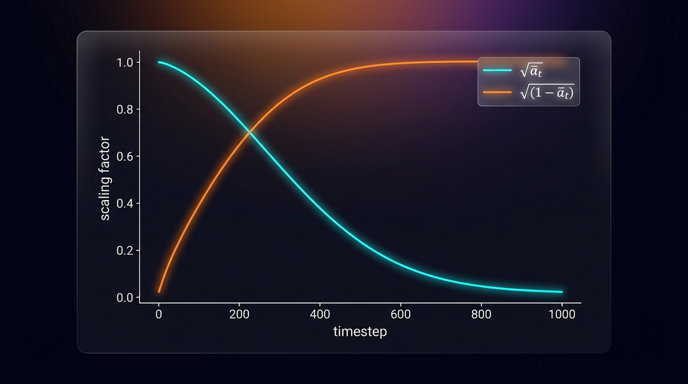
\(\sqrt{\bar{\alpha}_t}\) (signal, solid) starts near 1 and falls to 0. \(\sqrt{1-\bar{\alpha}_t}\) (noise, dashed) rises from 0 to 1. They cross at \(t \approx 250\) for a linear schedule — the point of equal signal and noise.

fig, ax = plt.subplots(1, 1, figsize=(10, 6))

plot_scheduler(DDPMScheduler(beta_schedule="linear"), label="default (linear)", ax=ax)
plot_scheduler(DDPMScheduler(beta_schedule="squaredcos_cap_v2"), label="cosine", ax=ax)
plot_scheduler(DDPMScheduler(beta_start=0.001, beta_end=0.003), label="low beta_end (0.003)", ax=ax)
plot_scheduler(DDPMScheduler(beta_start=0.001, beta_end=0.1), label="high beta_end (0.1)", ax=ax)

ax.set_title("Comparison of Noise Schedules")
ax.legend(fontsize=8, ncol=2)
plt.tight_layout()
plt.show()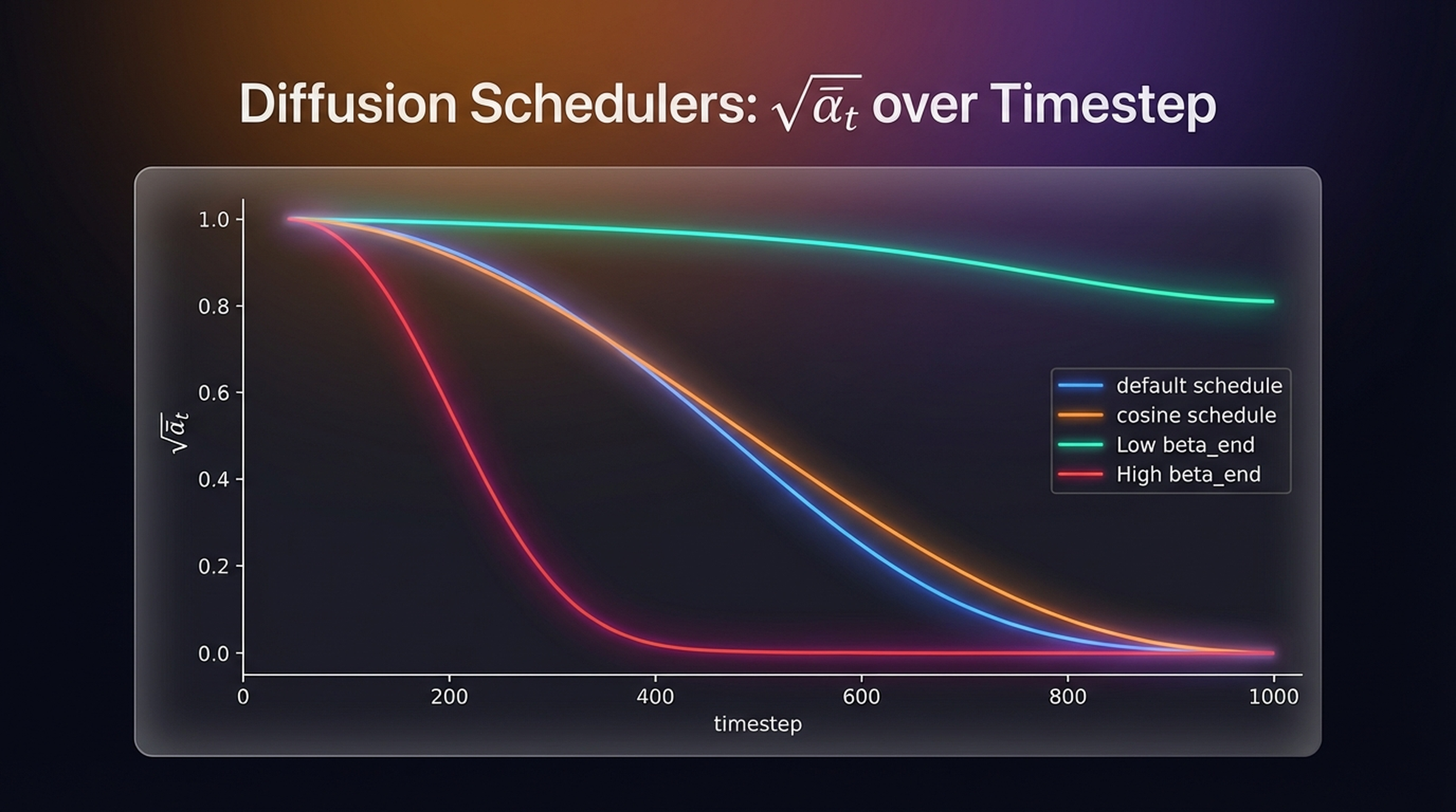

Four schedule configurations. Low beta_end: signal never fully collapses — inference breaks. High beta_end: signal collapses too fast — most timesteps carry no useful gradient. Cosine schedule is the recommended default.

9.4 Cold Diffusion — Beyond Gaussian Noise

Gaussian noise is the standard corruption, but the Cold Diffusion paper (2022) showed that the framework generalizes to any reversible corruption process.

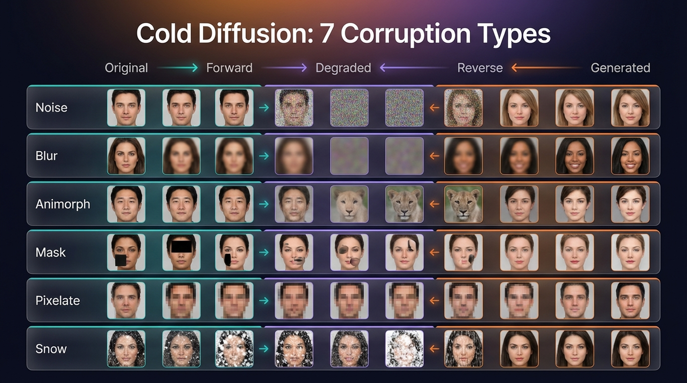
Cold Diffusion demonstrates that diffusion training works with blur, masking, pixelation, and other corruptions — not just Gaussian noise. The model learns to reverse whatever destruction process it was trained on.

10. Effect of Resolution and Input Scaling

The same noise level looks dramatically different at different resolutions. A high-resolution image has redundant information — neighboring pixels can reconstruct corrupted ones. A 64×64 image has no such redundancy. Noise at \(t=500\) destroys far more information at low resolution than at high resolution.

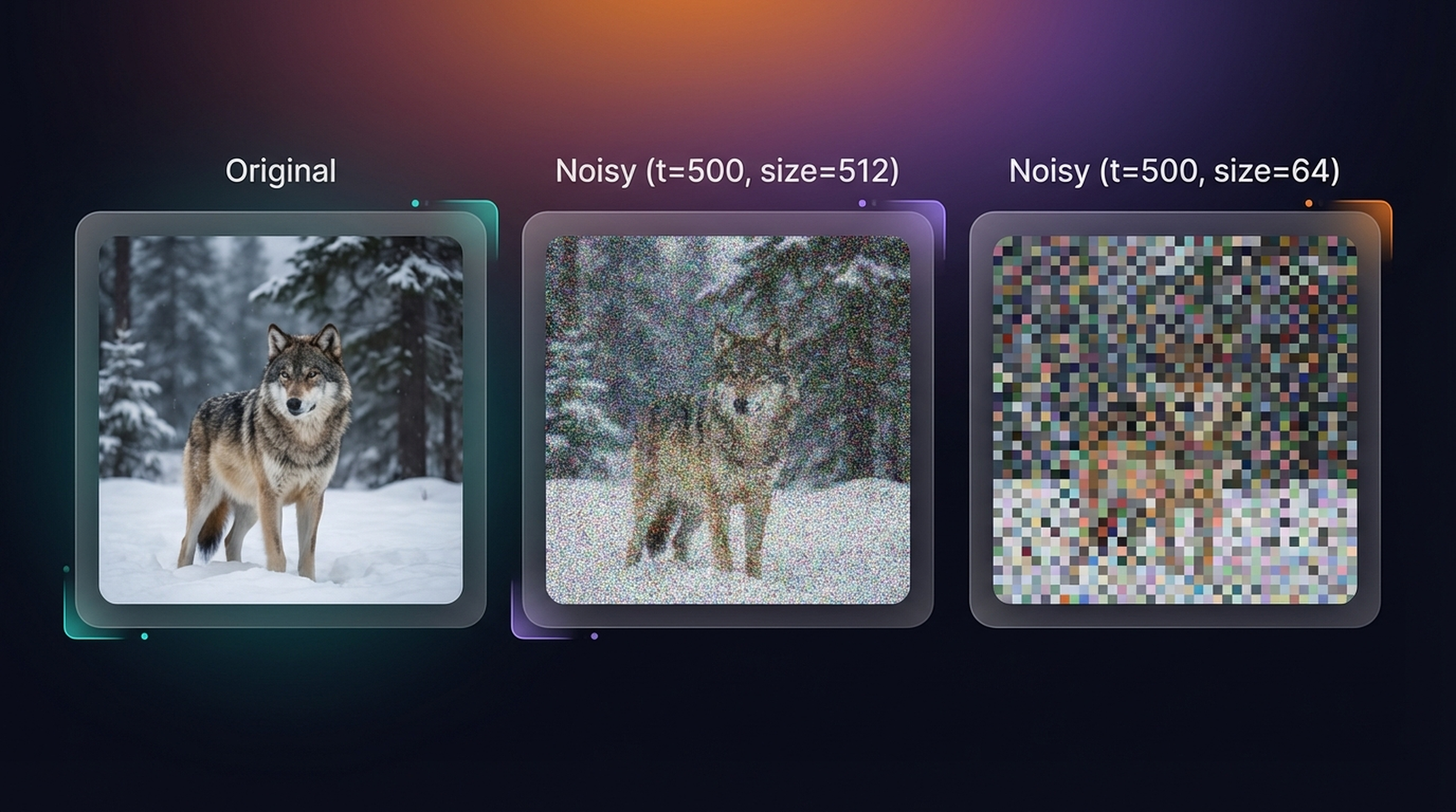
The same \(t=500\) noise level at 512×512 vs 64×64. The low-res version is nearly destroyed; the high-res version still shows clear structure. Schedules optimized for 64×64 training will perform poorly if applied directly to 512×512 inference.

Input scaling creates a related problem. If pixel values are in \([-1, 1]\) but we scale them to \([-0.1, 0.1]\), the noise immediately dominates. The Simple Diffusion paper (2023) proposed adjusting the noise schedule as a function of image resolution to compensate.

scales = [1.0, 0.7, 0.4, 0.1]
scaling_scheduler = DDPMScheduler(beta_end=0.05, beta_schedule="scaled_linear")
t = torch.tensor([500])
image_tensor = transforms.ToTensor()(pil_image.resize((64, 64)))
noise = torch.randn_like(image_tensor)

fig, axes = plt.subplots(1, len(scales) + 1, figsize=(14, 3))
axes[0].imshow(image_tensor.permute(1,2,0)); axes[0].set_title("Original"); axes[0].axis("off")

for i, s in enumerate(scales):
    scaled_input = s * (image_tensor * 2 - 1)
    noised = scaling_scheduler.add_noise(
        scaled_input.unsqueeze(0), noise.unsqueeze(0), t
    ).clip(-1,1) * 0.5 + 0.5
    axes[i+1].imshow(noised[0].permute(1,2,0).clip(0,1))
    axes[i+1].set_title(f"Scale={s}"); axes[i+1].axis("off")

plt.tight_layout(); plt.show()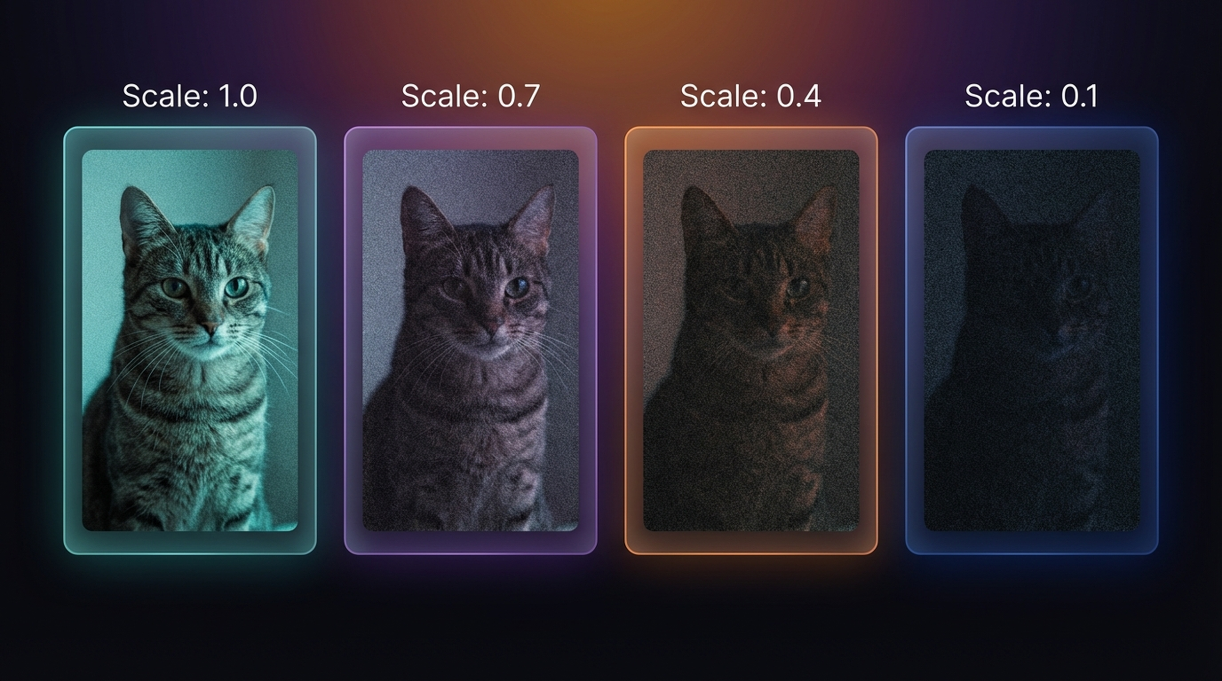

Same noise level \(t=500\), different input scales. At scale=0.1 the image signal is completely overwhelmed — noise dominates from the very first timestep.

11. UNets In Depth

To understand what makes the diffusers UNet powerful, we first build a minimal one from scratch and train it on Fashion-MNIST.

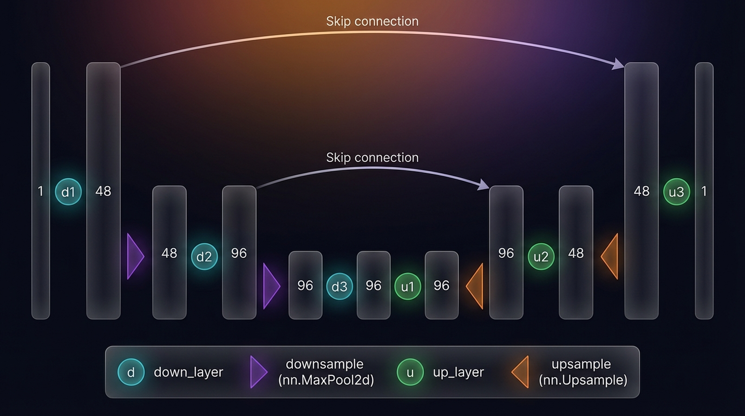
The BasicUNet. Three down-convolutions with MaxPool2d, three up-convolutions with nn.Upsample, skip connections via element-wise addition, SiLU activations throughout.

from torch import nn

class BasicUNet(nn.Module):
    def __init__(self, in_channels=1, out_channels=1):
        super().__init__()
        self.down_layers = nn.ModuleList([
            nn.Conv2d(in_channels, 32, kernel_size=5, padding=2),
            nn.Conv2d(32, 64, kernel_size=5, padding=2),
            nn.Conv2d(64, 64, kernel_size=5, padding=2),
        ])
        self.up_layers = nn.ModuleList([
            nn.Conv2d(64, 64, kernel_size=5, padding=2),
            nn.Conv2d(64, 32, kernel_size=5, padding=2),
            nn.Conv2d(32, out_channels, kernel_size=5, padding=2),
        ])
        self.act = nn.SiLU()
        self.downscale = nn.MaxPool2d(2)
        self.upscale = nn.Upsample(scale_factor=2)

    def forward(self, x):
        h = []
        for i, l in enumerate(self.down_layers):
            x = self.act(l(x))
            if i < 2:
                h.append(x)
                x = self.downscale(x)
        for i, l in enumerate(self.up_layers):
            if i > 0:
                x = self.upscale(x)
                x += h.pop()
            x = self.act(l(x))
        return x


basic_net = BasicUNet()
print(f"Parameters: {sum(p.numel() for p in basic_net.parameters()):,}")
print(f"Output: {basic_net(torch.randn(1,1,28,28)).shape}")  # (1, 1, 28, 28)

Note that for BasicUNet we use the x₀ objective — it predicts the clean image directly rather than the noise. Simpler to implement but, as we will see in Section 12, has weaknesses at high noise levels.

from torchvision.datasets import FashionMNIST

fashion_dataset = FashionMNIST(
    root="./data", train=True, download=True,
    transform=transforms.Compose([
        transforms.ToTensor(),
        transforms.Normalize([0.5],[0.5])
    ])
)
fashion_loader = DataLoader(fashion_dataset, batch_size=128, shuffle=True)

basic_model = BasicUNet().to(device)
basic_optimizer = torch.optim.Adam(basic_model.parameters(), lr=1e-3)
basic_losses = []

for epoch in range(5):
    for batch_imgs, _ in fashion_loader:
        x = batch_imgs.to(device)
        noise = torch.randn_like(x)
        amount = torch.rand(x.shape[0], device=device)
        noised = corrupt(x, noise, amount)
        pred = basic_model(noised)
        loss = F.mse_loss(pred, x)   # x0 objective
        basic_losses.append(loss.item())
        loss.backward(); basic_optimizer.step(); basic_optimizer.zero_grad()
    print(f"Epoch {epoch+1}/5, Loss: {basic_losses[-1]:.4f}")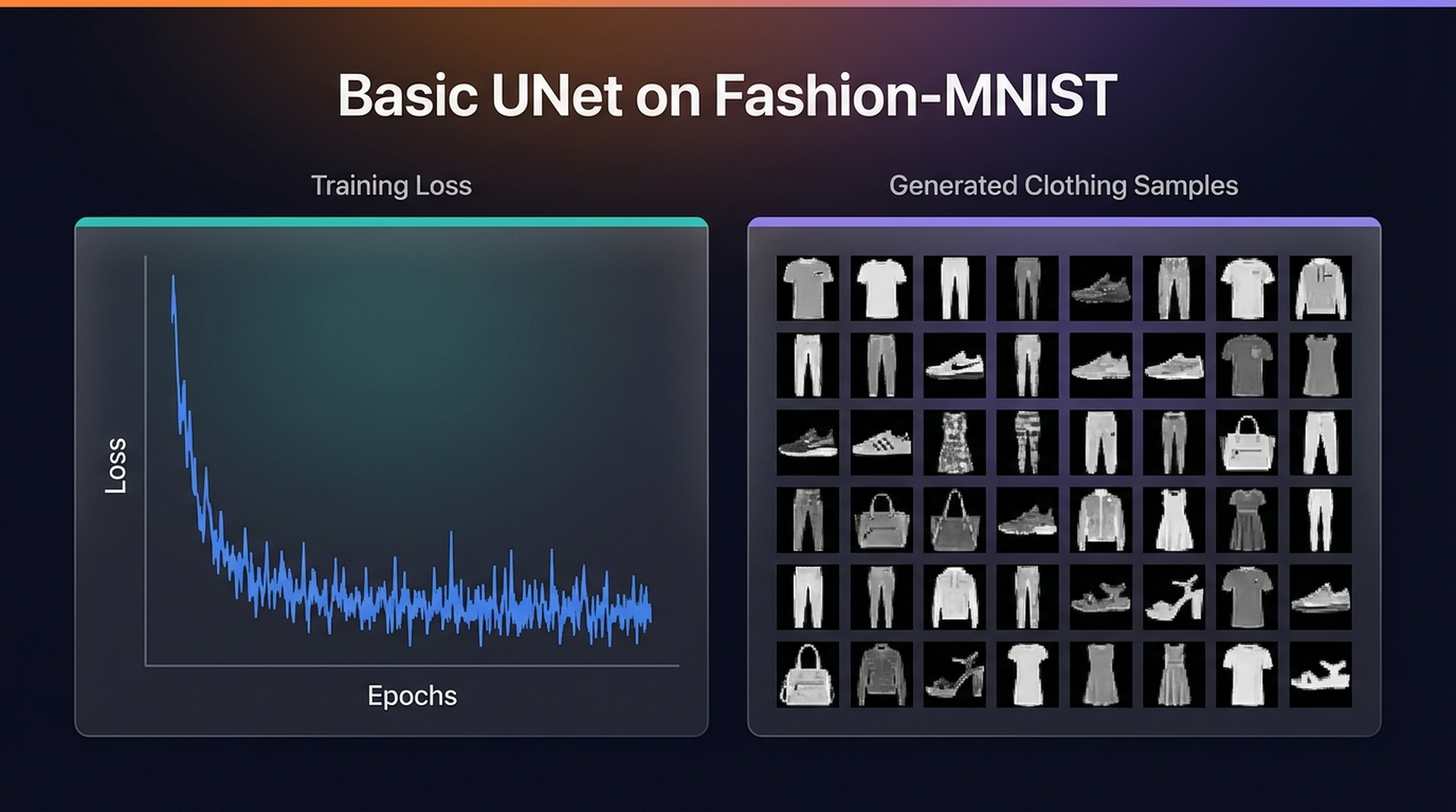

BasicUNet trained 5 epochs on Fashion-MNIST. Generations are recognizable as clothing items but blurry — no attention blocks, no timestep conditioning, no batch normalization.

The diffusers UNet2DModel upgrades the BasicUNet with attention blocks at lower resolutions, residual connections, sinusoidal timestep embedding, GroupNorm, and significantly more parameters.

advanced_model = UNet2DModel(
    in_channels=1, out_channels=1, sample_size=28,
    block_out_channels=(32, 64, 64),
    down_block_types=("DownBlock2D", "AttnDownBlock2D", "AttnDownBlock2D"),
    up_block_types=("AttnUpBlock2D", "AttnUpBlock2D", "UpBlock2D"),
).to(device)

fashion_scheduler = DDPMScheduler(num_train_timesteps=1000, beta_start=0.0001, beta_end=0.02)
adv_optimizer = torch.optim.AdamW(advanced_model.parameters(), lr=1e-4)
adv_losses = []

for epoch in range(10):
    for batch_imgs, _ in fashion_loader:
        x = batch_imgs.to(device)
        noise = torch.randn_like(x)
        t = torch.randint(0, 1000, (x.shape[0],), device=device).long()
        noisy = fashion_scheduler.add_noise(x, noise, t)
        pred = advanced_model(noisy, t, return_dict=False)[0]
        loss = F.mse_loss(pred, noise)   # epsilon objective
        adv_losses.append(loss.item())
        loss.backward(); adv_optimizer.step(); adv_optimizer.zero_grad()
    print(f"Epoch {epoch+1}/10, Loss: {adv_losses[-1]:.4f}")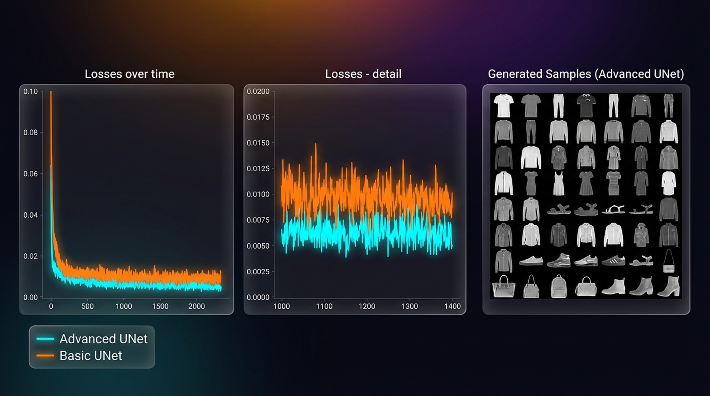

The advanced UNet produces sharper, more coherent clothing items. The loss gap is stark — the advanced model reaches ~0.05 MSE vs ~0.35 for BasicUNet. Timestep conditioning is the single most impactful addition: without knowing \(t\), the model cannot calibrate how aggressively to denoise.

12. Diffusion Objectives — ε vs x₀ vs v

What should the model predict? There are three common choices, each with different properties across noise levels.

The epsilon objective (predict the noise ε) is the DDPM default. It works well at high noise levels where noise is the dominant component. At very low noise levels (\(t \approx 0\)), the noise is so small it becomes trivially easy to predict — but also nearly irrelevant since we are already close to the clean image.

The x₀ objective (predict the clean image) is the opposite: easy at low noise levels where the image is visible, impossible at high noise levels (\(t \approx 1000\)) where a single noisy pixel carries no information about the specific original x₀.

The v-prediction objective predicts a velocity \(v = \sqrt{\bar{\alpha}_t} \cdot \varepsilon – \sqrt{1-\bar{\alpha}_t} \cdot x_0\) that balances both extremes. It avoids the pathological cases of pure epsilon and pure x₀ prediction, and is gaining adoption in modern architectures.

x0_demo = batch["images"][:1].to(device)
eps_demo = torch.randn_like(x0_demo)
demo_timesteps = [0, 199, 399, 599, 799, 999]

fig, axes = plt.subplots(4, len(demo_timesteps), figsize=(16, 9))
row_labels = ["Noised xt", "Target: eps (noise)", "Target: x0 (clean)", "Target: v (velocity)"]

for col, t_val in enumerate(demo_timesteps):
    alpha_bar = noise_scheduler.alphas_cumprod[t_val]
    sqrt_alpha = alpha_bar.sqrt()
    sqrt_one_minus = (1 - alpha_bar).sqrt()
    x_t = sqrt_alpha * x0_demo + sqrt_one_minus * eps_demo
    target_v = sqrt_alpha * eps_demo - sqrt_one_minus * x0_demo

    for row, target in enumerate([x_t, eps_demo, x0_demo, target_v]):
        img = (target[0].cpu().permute(1,2,0)*0.5+0.5).clip(0,1)
        axes[row, col].imshow(img); axes[row, col].axis("off")
        if row == 0: axes[row, col].set_title(f"t={t_val}", fontsize=10)
    if col == 0:
        for row in range(4):
            axes[row, 0].set_ylabel(row_labels[row], fontsize=9, rotation=0, labelpad=80)

Row 1: noised \(x_t\). Row 2: epsilon target (the noise). Row 3: \(x_0\) target (the clean image). Row 4: v-target. At \(t=0\) the noise target is nearly zero — trivially easy. At \(t=999\) the \(x_0\) target is pure noise — impossible to predict. The v-target remains a meaningful signal throughout.

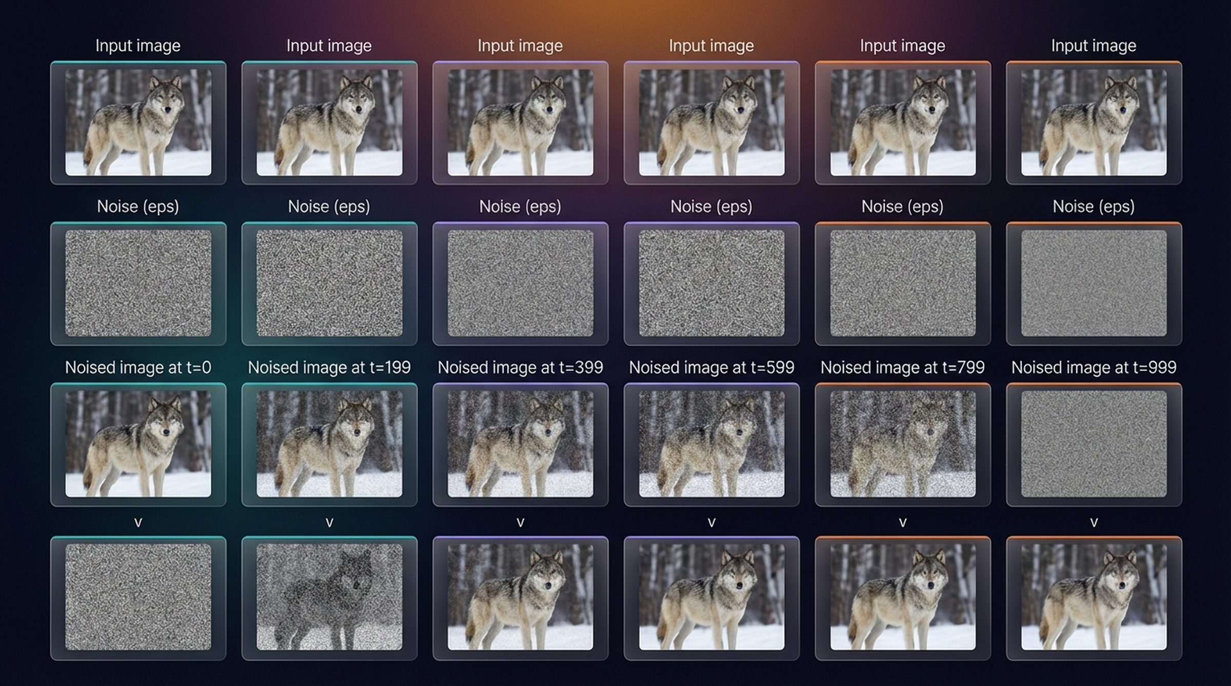
Complete breakdown: the clean input, the sampled noise, the noised image at each timestep, and the v-target. The v-target at \(t=0\) is nearly the noise; at \(t=999\) it is nearly the negative clean image.

13. Alternative Architectures

The UNet has been the default backbone for diffusion models since DDPM (2020), but the field is moving. Diffusion Transformers (DiT) replace the UNet entirely with a transformer operating on image patches — used in Flux, Stable Diffusion 3, PixArt-Σ, and Sora. They scale better with model size and training compute, following the same scaling laws as language models.

UViT is a hybrid: UNet-style outer blocks with transformer middle blocks, as proposed in the Simple Diffusion paper. RIN (Recurrent Interface Networks) maps the image to a lower-dimensional latent space, processes it with a transformer, then decodes back — reducing the quadratic attention cost of operating at full resolution.

The UNet remains dominant in production (Stable Diffusion 1.x, 2.x) due to its maturity and efficiency at 64×64 resolution. For higher-resolution and text-conditional generation, transformer-based architectures are increasingly preferred. If you read our previous post, you already have everything you need to understand DiT: it is simply a Vision Transformer applied to noisy latent patches at each denoising timestep, conditioned on the timestep and class label via adaptive layer norm.

14. Summary

Diffusion models solve the single-shot problem of GANs and VAEs by replacing one difficult generation step with 1000 easy denoising steps. Each step asks only: what noise was added here? Learned across all noise levels simultaneously, this produces a model that can generate novel, high-quality images from pure Gaussian noise.

The complete pipeline we built:

Forward process: \(x_t = \sqrt{\bar{\alpha}_t} \cdot x_0 + \sqrt{1-\bar{\alpha}_t} \cdot \varepsilon\) — jump to any noise level without iteration.

Reverse process: Start from \(x_T \sim \mathcal{N}(0, I)\), apply UNet at each timestep to predict ε, use scheduler to update \(x_{t-1}\). Repeat 1000 times.

UNet: Same-shape input/output, encoder-decoder with skip connections. Modern versions add attention at low resolutions, residual blocks, sinusoidal timestep embedding, GroupNorm.

Training: MSE between predicted and actual noise (epsilon objective). Random timesteps per batch — the model must handle all noise levels.

Noise schedule: Linear or cosine \(\beta_t\) progression. Cosine is generally preferred. Getting beta_end wrong (too low or too high) hurts both training and inference.

Main tradeoff vs GANs: Inference is slow — 1000 model forward passes per image. This spawned an entire line of research into accelerated samplers (DDIM, DPM-Solver, LCM) that reduce this to 20–50 steps without significant quality loss.

The next post builds on everything here to add conditioning — guiding the denoising process with text, class labels, or other signals. That is the path to Stable Diffusion, DALL·E 2, and modern text-to-image generation.

That covers our deep dive into diffusion models — from pure noise to generated images, with the math fully unpacked. Take care! 🙂

References

[1] dH #010 — Understanding Diffusion Models Through 1D Experiments, datahacker.rs

[2] Foster, D. — Generative Deep Learning: Teaching Machines To Paint, Write, Compose, and Play, 2nd Ed., Chapter 4. O’Reilly Media, June 2023. ISBN 978-1-098-13418-1.