Highlights: Hello and welcome back. In this post, we will see how we can use Neural Networks for the segmentation task. To be more precise, it will be about Semantic Segmentation. The goal of Semantic Segmentation is to label each pixel of an image with a corresponding class. We will cover some of the most popular Deep Learning models for segmentation:

• Fully Convolutional Neural Network
• SegNet
• U-Net

Tutorial Overview:

• What is Semantic Segementation?
• Types of segmentations
• Fully Convolutional Neural Network for Semantic Segmentation
• SegNet – Autoencoder-Decoder segmentation network
• U-Net

1. What is Segmentation?

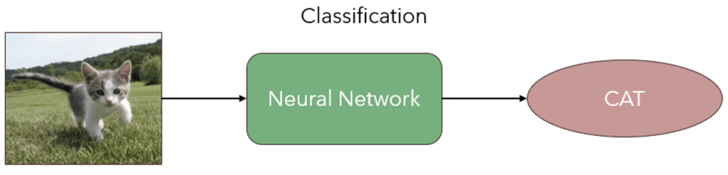
When we start to learn Deep Learning our first experiments are tasks that are usually related to solving classification problems. We need to determine the class label of the object in the image. For instance, we have a cat or non-cat images.

Then as we progress, we encounter problems such as object detection. The difference is that apart from the need to determine the class label we also need to determine the position of the bounding box that implies where the object is. For instance, we can place a bounding box around a cat, and in this way, we have localized the cat in the image.

And then, there are tasks when we need to be even more precise when processing images. Imagine that you have an image of yourself and you want to change the background on your photo. In this case, you need a very precise edge/contour detection that will segment and label all pixels that belong to your body.  The output image of the segmentation process should label all the pixels that belong to your body as a unique label class.

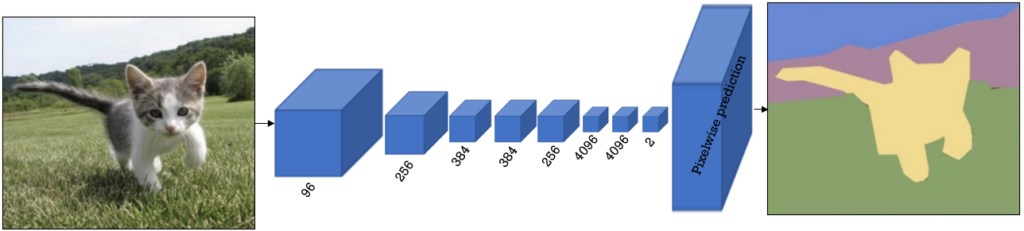
To illustrate this a little bit better, have a look at the image below. The goal of the segmentation is to create an image of the same size as the input image. The pixels of the new image should belong to one out of four groups:

1. Cat
2. Grass
3. Mountain
4. Sky

2. Types of segmentations

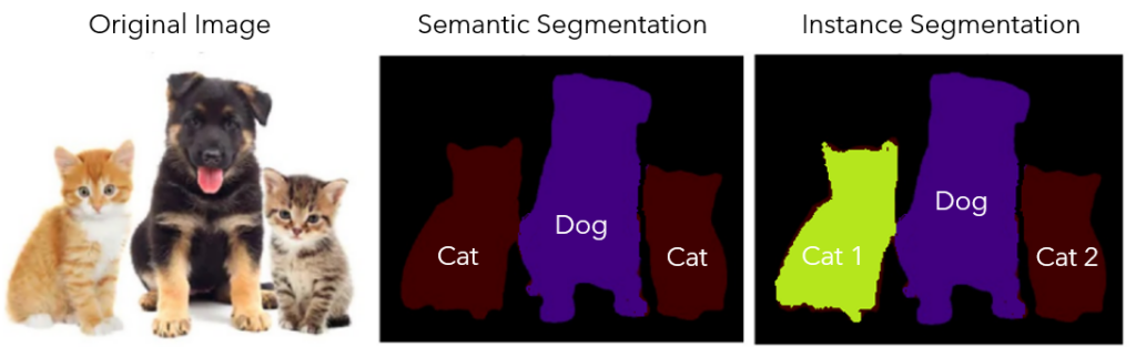
When we perform a segmentation there are two types:

1. Instance Segmentation
2. Semantic Segmentation

For example, a cat can be seen as an instance. If there are two cats in an image, if we perform semantic segmentation, both cats should be represented with the pixels from the same class label. But, if we are interested in separating every single object instance we are performing instance segmentation.

When to perform semantic segmentation?

In case that we are also interested in segmenting objects that are not instances. Such objects are the sky or grass.

How do we train a neural network to achieve this?

Our goal for this would be to train a neural network for segmentation steps. This training should enable us to produce an output image of the same size as the input image. And yet, the pixels of the output image should represent class labels of objects that are detected in the input image. 

Note that in the image above we have illustrated a semantic segmentation. In case that we have used instance segmentation, and we had two cats in the image, they would be represented as two different label classes.

Now, let’s see some methods and algorithms for semantic segmentation. Note that we are just going to explain the basics of how these algorithms work and not the full theoretical concept. We will explain them in future posts in more detail, so stay tuned for that.

3. Fully Convolutional Neural Network for Semantic Segmentation

Fully Convolutional Neural Networks that we have commonly used for classification can be used for Semantic Segmentation as well. Obviously, later we will discuss more advanced models for segmentation, but historically we will start with the first paper that employed deep learning architectures [Long et al., 2015].

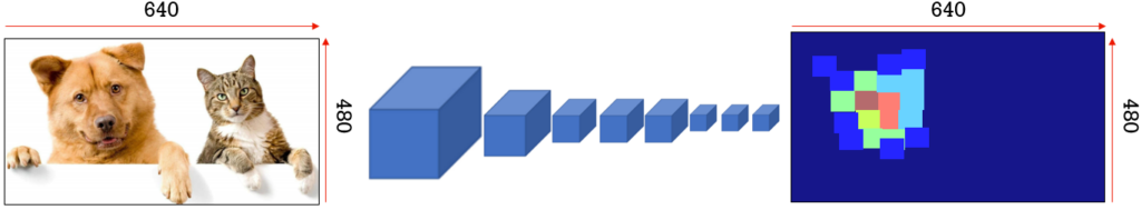
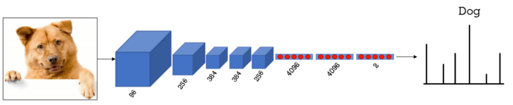
Usually, a network starts with a series of convolutional layers, and then, we have several fully connected layers at the end. However, to solve the problem of semantic segmentation, we need to modify the final layers. This means that instead of a classification output (e.g. softmax layer), we will have an image of the same size as the input. 

In a CNN the image size, that is, the number of pixels will decrease as we propagate through the network. Therefore, we need to adjust our network in order to perform segmentation. The most important steps would be:

• Replacing the fully connected layers with the convolutional layers

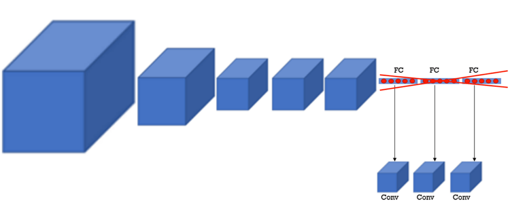
• The last layer would be modified in such a way that the output matches the size and resolution of the input image.

• The loss will be calculated in a pixel wise manner between the predicted output of the network and the ground truth labelled image. 

One way to convert fully connected layers into convolutional layers is to use a 1×1 convolution. This process is known as a ‘convolutionization’. If you need to refresh your knowledge on 1×1 convolution, we have already explained that in the following post.

So, what did we achieve by making these modifications?

Well, we went from a standard classification model to a segmentation model. We don’t get probabilities of what is in an image, but rather, we get an image that represents what and where it is on the input image. What would happen if we trained our model to only detect dogs, but in the image, a cat appears. The model would then segment that image and return the segmentation map with only the dog segmented.

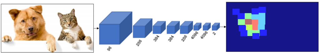
In addition, this research work proposed to use different levels for the segmentation. In the image above, high-level features are used to obtain a heatmap. However, to better predict the edges and contours of the objects, the low and intermediate-level features are also used. Recall that the first layers in the convolutional networks learn to recognize and detect edges. 

Hence, a combination of high, coarse, layers with low and fine layers obtains an improved segmentation accuracy.

4. SegNet – Autoencoder-Decoder segmentation network

The next interesting semantic segmentation network is the so-called SegNet. This approach represents a further improvement in the segmentation-related networks and it uses the well-known autoencoder-decoder architectures to develop a neural network.

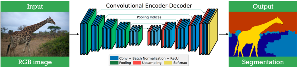
The first part of the network is the classical CNN that consists of convolutional layers and max-pooling layers. In addition, it uses batch normalization layers as well as ReLU activation functions. These layers are often used in Deep Learning.

The second part, the right part of the network, is the so-called decoder part. The main goal of the decoder is to upsample the output from the encoder part to obtain a new image. This part is created using upsampling layers and convolutions. These parts are also trained using backpropagation. The process of upsampling can be done using transposed convolution.

What exactly is a transposed convolution?

Transposed Convolution

The main goal of transposed convolutions is to increase the size of a feature map, from a smaller size to a bigger one.

Looking at the example above, we want to change the shape from a 3×3 up to a 5×5 output feature map. The image that we want to upsample are the blue squares at the bottom. The process of a transposed convolution consists of the following steps:

• We will zero pad the original image, 3×3, and place the paddings on all sides of the pixels. These are represented as the white squares. This way we went from the original 3×3 image to a 7×7 image that is zero padded image.
• Then, we will have a 3×3 convolution filter (kernel) that we will use to produce our output. Note that this filter is shown as a gray square (3×3) that is moving accross the image.
• By moving the kernel, we can see that at that particular position, it will generate one output element (pixel) of the output feature map on the top (5×5).

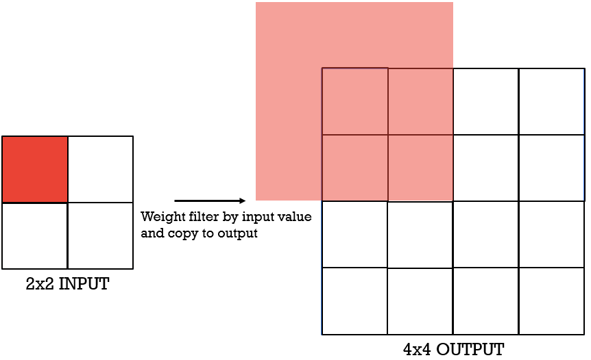
To better illustrate this concept, let’s look at a simpler example. Now, assume that we have a 2×2 feature map that we want to upsample to a 4×4 feature map using transposed convolution. 

In simple words, the transposed convolution in this case will just scale the filter, that is of size 3×3, elements and place them in the output. This is illustrated using a 3×3 red square. That is, the filter coefficients are multiplied with the single element depicted in red in the input 2×2 feature map, and these values are stored in the output, where the red square is.

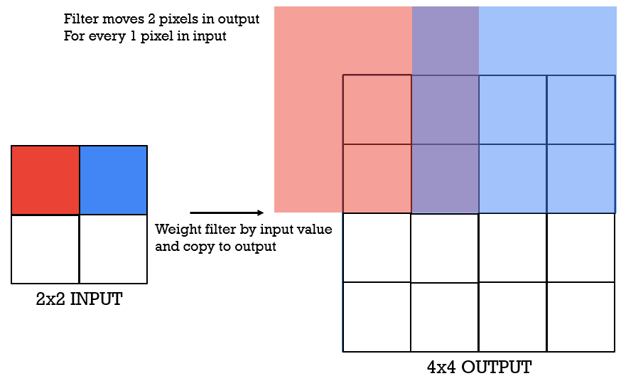
We will be using a stride of 2, which means that our kernel will move 2 pixels on the right.

Next, as we move our filter to process the element colored in blue, we will again multiply the filter coefficients with this value. Then, we will store the result in the output feature map as shown with a blue 3×3 square.

You might notice that there is an overlapping column between the red and blue squares in the output image. How can we solve this problem?

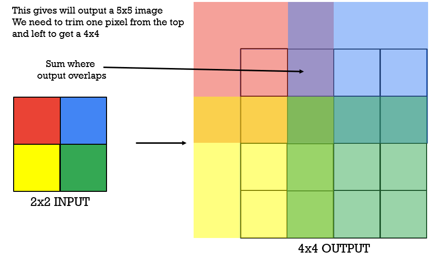
Simple enough, we will sum these values and store them accordingly.

Finally, we will repeat this process until we have covered all the pixels in the 2×2 input image and obtain the following output image (5×5).

Now, as you can see the final output image has a pixel that is the intersection of all four squares. This value will be obtained by four summations of the scaled filter coefficients. And at the end, we have actually obtained a 5×5 output image, but we will trim it to obtain the final 4×4 output image. We will trim the pixels on the left and on the top to obtain the 4×4 output image.

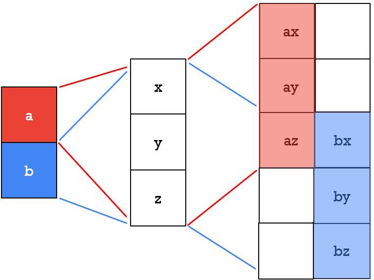
Maybe you ask yourself. This is for a 2D transposed convolution, but what about 1D?

Well, it is pretty similar. To illustrate this, we will assume that our input signal has 2 elements (a, b) and that we have a filter of length 3 (x, y, z). Again, the stride in the output signal will be 2 and this is represented in the image below.

We multiply each pixel with the kernel, filter, and obtain the image on the right. Note, once again, we have an element that is intersecting. This value will represent a summation (az + bx).

SegNet has one additional detail that is very interesting to mention here. It is called “max unpooling”. It actually starts with the pooling process. During the max-pooling process, we usually perform max() operation. These maximum positions are saved and can be used in the process of max unpooling. The concept is fairly simple and is illustrated in the image below. 

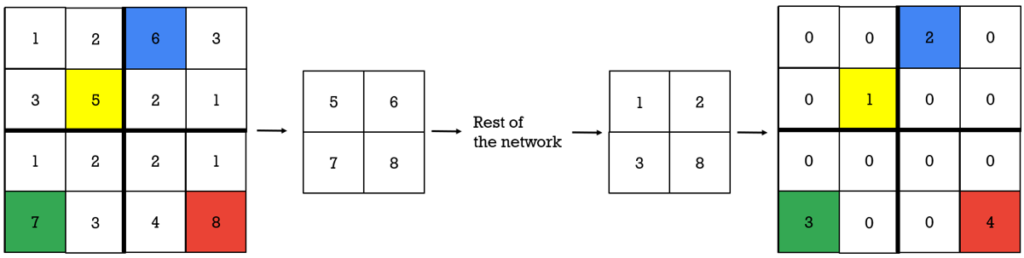
The indexes of the maximum position are shown on the left and highlighted in color. Then, if we have a different matrix (elements 1,2,3,4) we perform max unpooling in a way that we place those elements at the previously remembered maximum locations, and then, we zero pad the remaining fields. This is illustrated as the matrix on the right part of the image above.

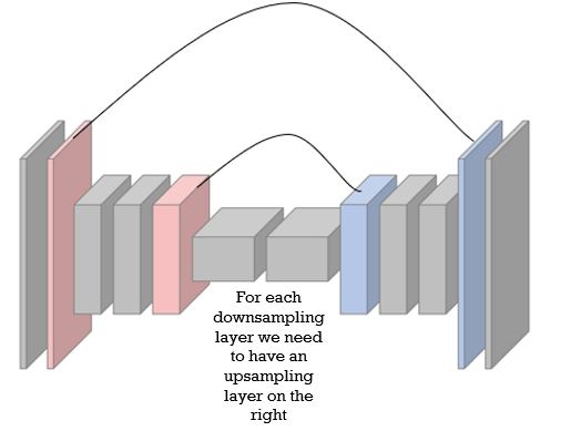
One thing that we also need to cover, is that each downsampling layer on the left (red) needs to have an upsampling layer (blue) on the right.

U-Net

Now, let’s see another segmentation model. We will talk about U-Net, skip connections, and autoencoders. Looking at the model architecture below, on the left part of the network we can see an encoder architecture, and on the right, we have a decoder architecture.

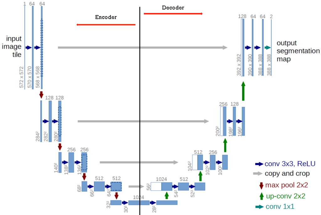
Looking at the shape of this model, we can see where it got its name from, U-Net. When this model was first proposed, It was created for image segmentation for biomedical images.

One interesting thing here is the gray horizontal connections between the encoder and decoder part in the network. These represent skip connections, and we will examine what they are.

The main idea behind the U-Net is that the decoder part, the right part of the network, is processing a lot of image data and basically compressing it into a bottleneck layer. These can be viewed as high-level pieces of information. Essentially, in the decoder, we are trying to add and recreate more and more detail.

As we progress through the encoder part, the left part of the network, more and more spatial information is lost. On the other hand, the low-level features are essential to determine the exact boundaries of the objects. So, the main goal of the skip connections is that they pass these low-level pieces of information and combine them with high-level pieces of information. In practice, for instance, in PyTorch, this combination of features is a simple concatenation of features.

Summary

Well, that’s it for today’s tutorial! We hope that you found this overview useful and that you now understand the basic ideas and architectures behind these algorithms. Once again, this was just an overview, more details about these algorithms will be covered in the upcoming posts. So, we‘ll see you soon with some more interesting algorithms.

References

1. Long, Jonathan, Evan Shelhamer, and Trevor Darrell. “Fully convolutional networks for semantic segmentation.” Proceedings of the IEEE conference on computer vision and pattern recognition. 2015.
2. Badrinarayanan, Vijay, Alex Kendall, and Roberto Cipolla. “Segnet: A deep convolutional encoder-decoder architecture for image segmentation.” IEEE transactions on pattern analysis and machine intelligence 39.12 (2017): 2481-2495.
3. Ronneberger, Olaf, Philipp Fischer, and Thomas Brox. “U-net: Convolutional networks for biomedical image segmentation.” International Conference on Medical image computing and computer-assisted intervention. Springer, Cham, 2015.
4. Vincent Dumoulin, Francesco Visin – A guide to convolution arithmetic for deep learning