#027 R-CNN, Fast R-CNN, and Faster R-CNN explained with a demonstration in PyTorch

Highlights: Object detection is one of the most important tasks in Computer Vision. In this post, we will give an overview of one of the most influential families of object detection algorithms: R-CNN, Fast R-CNN, and Faster R-CNN. We will highlight the main novelties and improvements for each of them.
Finally, we will focus on the Faster R-CNN and explore the code and how it can be used in PyTorch.
Tutorial Overview:
1. Introduction to object detection
The goal of object detection can be seen as an extension of the classification problem. In classification, we have one dominant instance or object in the image that occupies the central image area. Then, our goal is to detect what it is in the image.
Object detection is similar but more complex. First of all, we not only need to guess what it is in the image but also to detect its location. This is commonly done by positioning a rectangle box around the object-bounding box. This positioning is done with the respect to ground truth labeling. That is, the algorithm should learn the labeling process of the annotators and how exactly to place this rectangle box. In essence, this can be cast as a regression problem. On the other hand, the answer to what exactly in the image represents a classification problem.
For each object we are predicting:
- What is in the image? This is the classification task where we predict the category label
- Where is the object in the image? This is the Localization task where we predict the bounding box around the object (4 numbers: x, y, width, height)

To better illustrate this, we will review the classification using neural networks. For instance, we can have an AlexNet.
Detecting single objects

This network will tell us “What” is in the image. For that, we will get an output score probability vector. For instance, there is a 0.9 chance that there is a cat in the image.
This prediction is obtained from the “last” fully connected layer of size 4096 and fed into a softmax activation function. Subsequently, this vector can also be used for the generation of the answer “Where” a cat is in the image and this will be cast as the regression problem. Here, the regression output will be four values: x, y, width, and height.
As for the loss function for classification, it is well-known that we will use a cross-entropy loss. On the other hand, for the regression problem, we will use an L2 loss function.
Now, the problem is that we have two different losses. However, we need a single loss function to apply gradient descent and optimize parameters. Well, the solution proves to be fairly simple. We will sum the two losses. That is, to be more precise, we will use a weighted sum and adjust the weight parameters. The weight of the parameters will imply what out of the two terms is more valuable to us. On the other hand, this can simply be used to adjust the scale for both losses.
Hence, we have one network and we want to output multiple results. This is standard architecture in Computer Vision and it is called a Multitask Loss.
However, there is one huge problem. We can have more than one object in the image, and now things are getting more complex 🙁 So, we cannot exploit this idea of multitask loss.
Detecting multiple objects
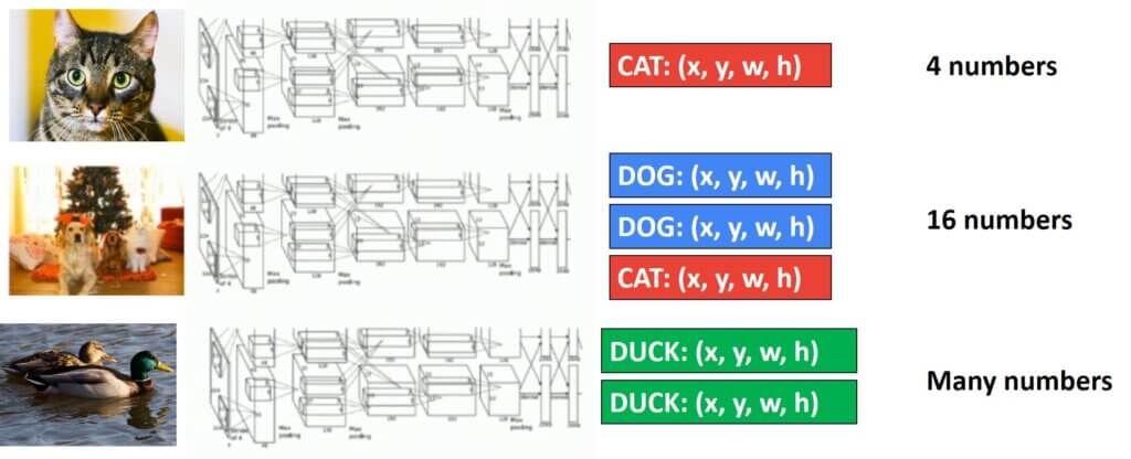
In the Figure above, we can see an example of detecting a large number of “ducks” (or some other bird that is in the image).
2. R-CNN
A solution is to use sliding windows of different sizes and aspect ratios.
Have a look at the image below:
Sliding window
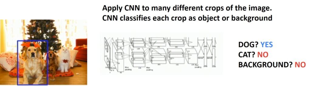
Then, once we select a sliding window, we treat this as a simple classification task. In other words, since we can have multiple numbers of different classes in the same image, we have removed a multitask learning loss function and removed the regression part. Now, we have cast our problem into:
- Finding a sliding window
- Performing a classification
The main problem that now exists is how we cover the whole image with sliding windows of different sizes and run a CNN detector for each of them. Well, it can be quite a lot of windows and we need to strategize in order to find an optimal solution.
Luckily, this “sliding window approach” is not a new problem in Computer Vision. We have already seen it in the face detection algorithm developed by Viola and Jones, 2001.
Region proposals:
- Find a small set of boxes that are likely to cover all objects.
- Often based on heuristics: e.g. look for “blob-like” image regions
- Relatively slow to run; e.g. Selective Search gives 2000 region proposals in a few seconds on CPU
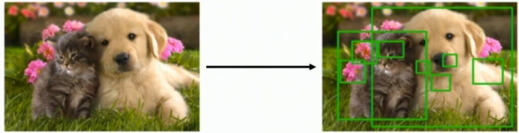
Other researchers have also explored this problem extensively and the main idea is to focus on finding “promising potential windows” for our image. For instance, we can search for blob-like patterns in the image, and find a small set of windows that will cover the whole image, just to name a few. In addition, the algorithm “Region proposal” is finally developed with an approach to detect 2,000 sub-regions for one image, with a high probability that they will overlap with the objects that we are searching to detect.

At last, we arrive at the definition of the R-CNN algorithm. Here, R stands for a region.
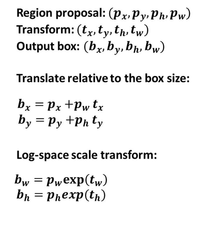
The algorithm finds 2,000 regions of interest (RoI). Next, the input image for each RoI is warped to size: \(224\times224 \). As the last step, a trained CNN is used to examine whether there is an object of interest present in the warped image region.
In addition, there is also a part of the network that refines the RoI. Here, the RoI is slightly adjusted so it gives us a sequence of 4 numbers: \(t_{x} \), \(t_{y} \), \(t_{w} \), \(t_{h} \). The following formula shows how we obtain the final output bounding box.
In case this is your first algorithm related to object detection, you may wonder how we measure accuracy. For classification it was rather easy, but what do we do for object detection?
For this, we use a concept called Intersection over Union – IoU.
Intersection over Union
How do we tell if our object detection algorithm is working well?
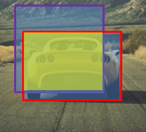
An intersection is a yellow region and a union is the whole blue region (including the intersection)
Imagine that the red bounding box is a ground truth label. Next, our detector outputs that there is a car present in the image as marked with the purple bounding box. IoU is then easily defined in the following image as a ratio between the intersection and the union between two bounding boxes.
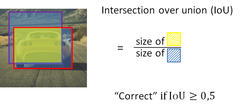
Commonly, values larger than 0.5 are considered good detections. In the ideal case, we would have a complete overlap and in that case, our IoU would reach a maximal value of 1.
Next, there is one more challenge when working with object detectors. In essence, there will be a large number of bounding box candidates for the same object in the image. Therefore, we do need an algorithm to tackle this problem. One popular algorithm for this is a non-maximum suppression – NMS.
Non-maximum suppression
The idea of this algorithm is fairly simple. Imagine that our detector gives us the following detections for two cars in the image below. In addition to each bounding box, we also have a probability score for the car class for that detection.

Well, the goal of the NMS is to keep first the object with the highest class probability. For instance, those would be two rectangles with probabilities: 0.8 for the left car and 0.9 for the right car. When we keep those with the largest probabilities, we will then search for the bounding boxes having the same class and high IoU as these bounding boxes. In our case, we will first select the right car (\(p=0.9 \)) and remove two overlapping red rectangles (over the car on the right). Similarly, we will repeat the same procedure for the car on the left, thereby leaving the white rectangle (\(p = 0.8 \)).
Mean Average Precision – mAP.
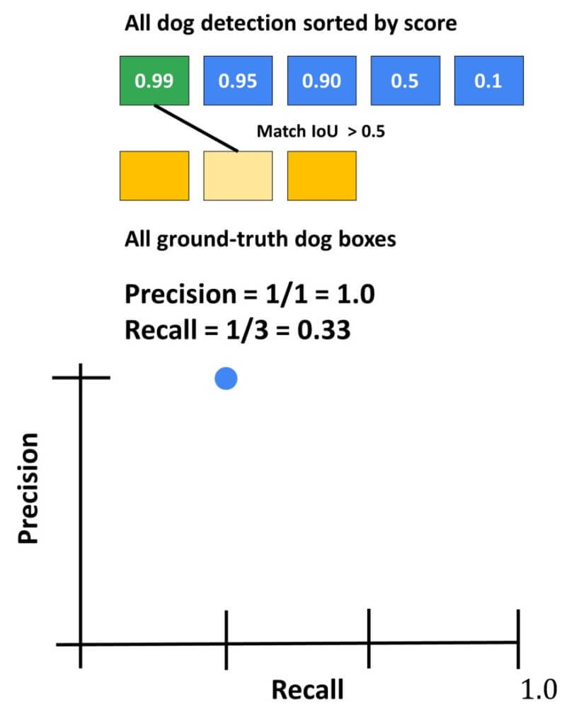
Finally, after processing our detections with IoU and NMS we need to calculate the accuracy of the object detectors. This is done with a metric called: Mean Average Precision – mAP.
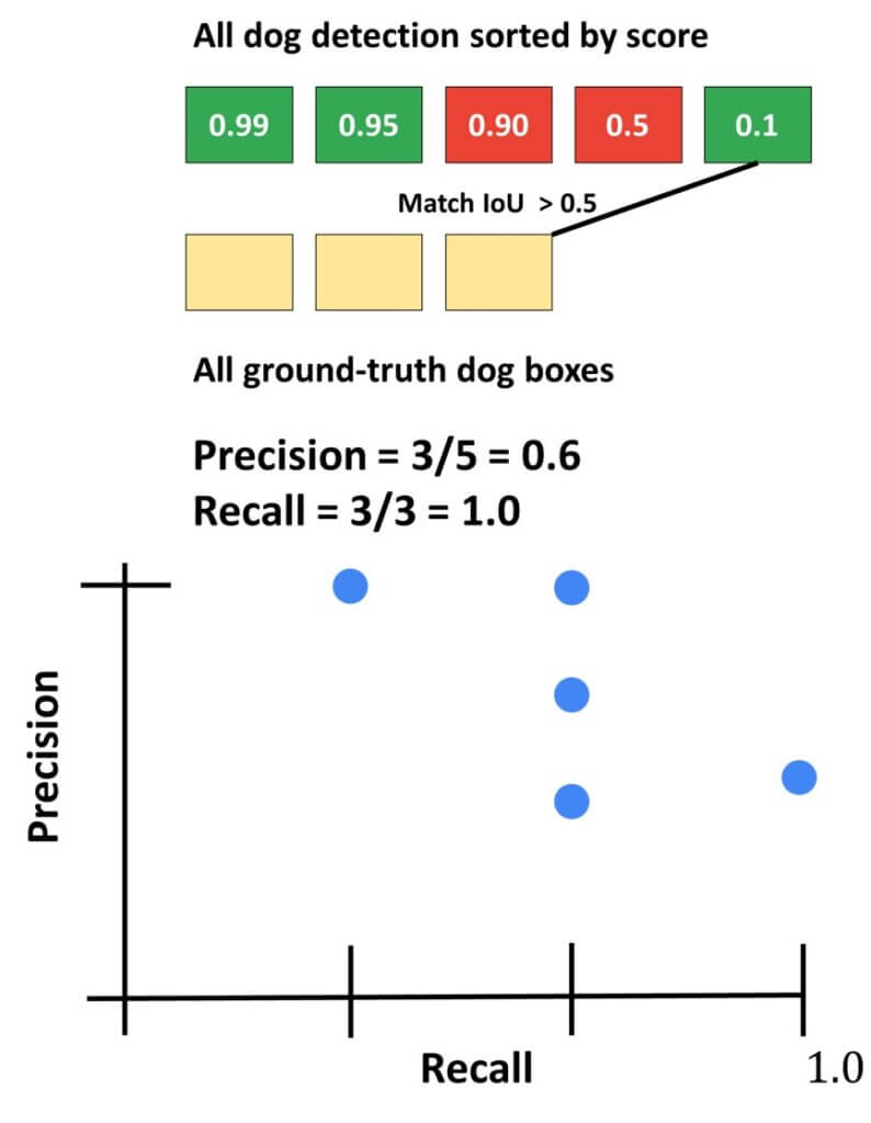
The steps to calculate mAP can be summarized as follows: we have detections for a “dog object”. Let’s say that in total we got 5 dog detections. However, we have only 3 ground truth detections. We will start with the highest class probability (p=0.99) and calculate IoU with ground truth detections. If we have a value higher, let’s say than 0.5, we will count it as a true detection. In this case, we calculate precision and recall iteratively. This can be easily visualized in the following Recall/ Precision graph.
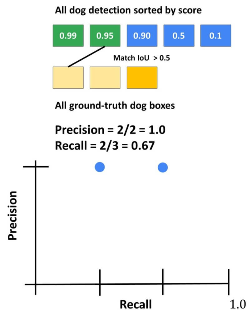
Then, we calculate the same for the second detection. For instance, it would be a match with the third ground truth detection. Now, we will again update the recall and precision and plot them accordingly.
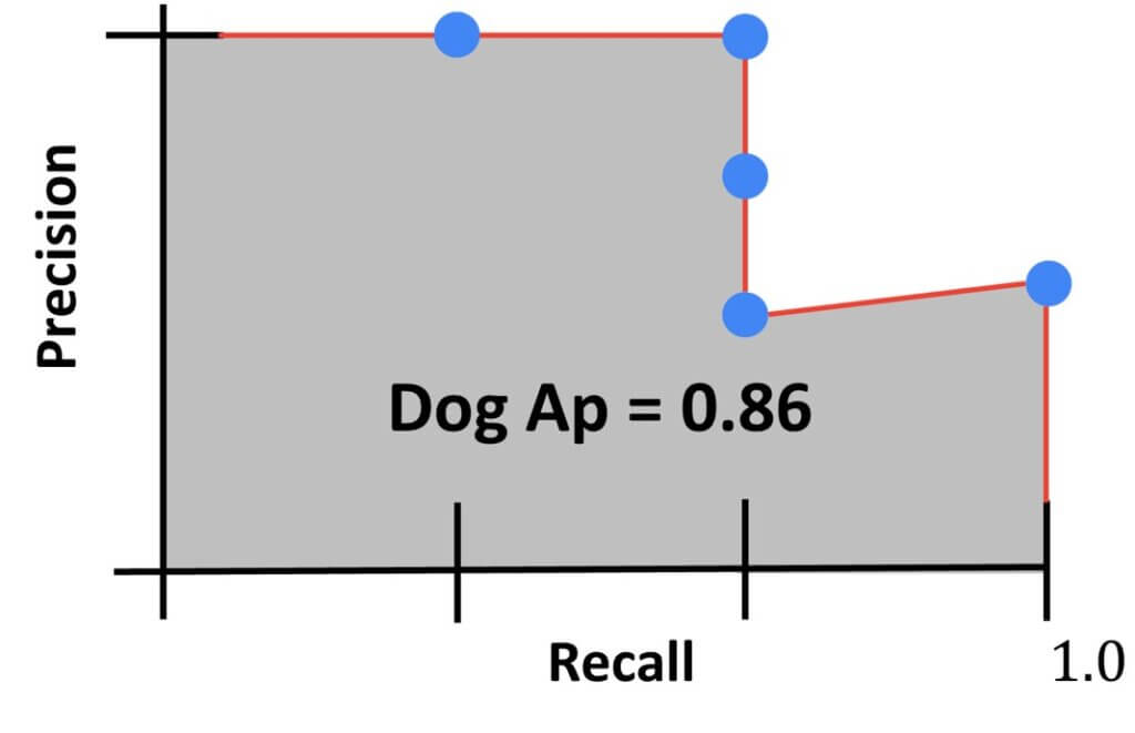
Next, we can imagine that the next two detections were actually false positives and that the final, fifth detection was true-positive. Then, the evolution of recall and precision would be as follows:
Finally, we output the final value for our dog detector. It will represent the area under the curve.
Then, for one object detector, imagine that we have three classes that we are detecting. We will calculate AP for all three classes and take an average over all three classes. Finally, we will obtain the meanAP or mAP.
3. Fast R-CNN
The R-CNN algorithm was an amazing object detector when it was invented. However, researchers quickly realized the major drawback of this algorithm. It was very very slow. So, today, sometimes people even refer to it as a slow R-CNN.
The improvement came from a rather simple idea. The processes of 1) warping and 2) running CNN on the warped image were swapped. Then, the running of backbone CNN is done only once and this will speed up things drastically.
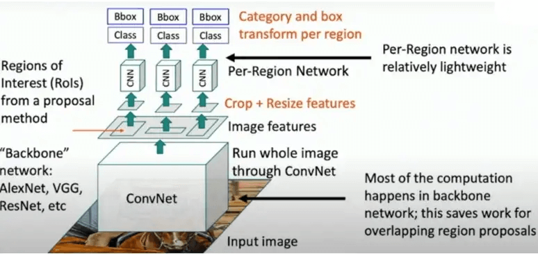
We will explain the term “backbone”. This is commonly a pre-trained AlexNet or VGG-like network. It will represent a basis for processing our object detector and this saves a lot of work. Next, the processed output will represent a feature map. Note that the backbone consists of convolutional layers including max pooling and batch normalization, but not of fully connected layers. Then, these feature maps will be adjusted to fit the ROIs and for that purpose, feature maps will be cropped/resized and warped. Next, we will process each of these sub-sets of warped features using a lighter “Per-Region Network”. This lighter network would be computationally much less demanding. For instance, this network may consist of only 2 last fully connected layers from the AlexNet.
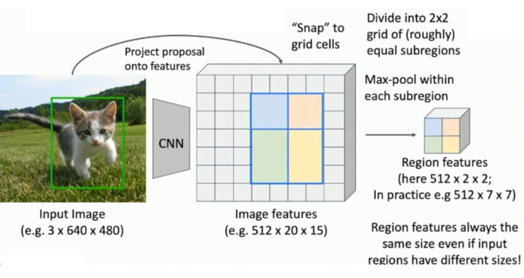
One question may still puzzle us. How do we actually crop features?
Imagine that we have the following processing pipeline:
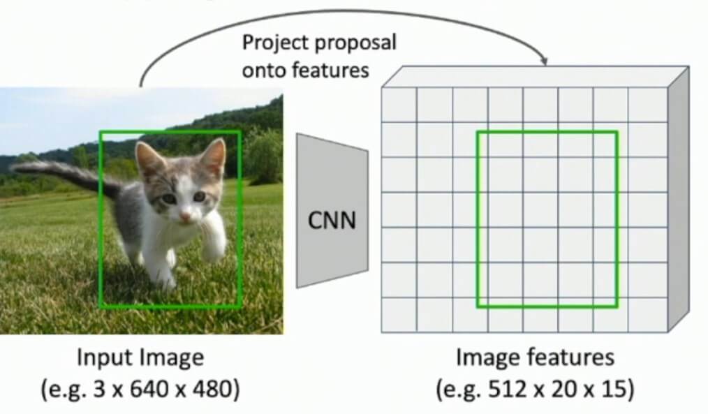
With the specified RoI (green rectangle over the cat) we will “snap” to the image feature maps and continue calculations as usual. Here, without going too much into detail, we will just demonstrate this process in the following image. In simple words, the algorithm will find the best match between the original RoI and the feature map elements. Where necessary the dimensions will be adjusted so that for instance in some cases we may have even \(3\times2 \) pooling region as shown in the image below.
This outlines the main ideas of the Fast R-CNN. And what is the gain?
Have a look at the following image:
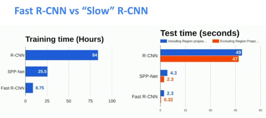
We can see the results that we will need to spend on training and also on the test time. This was a significant improvement in speed!
4. Faster R-CNN
We have arrived at the third algorithm in the series, Faster R-CNN. Again, the goal to create an even faster R-CNN algorithm can be seen in the following:
- Remove the selective RoI proposal algorithm
- Create a layer/network that will select RoI for us depending on the image that we are processing
This network is called Region Proposal Network (RPN). The goal is to generate feature map activations. Then, these features we will feed these to RPN and it will output the regions. Next, we perform everything within the Fast R-CNN.
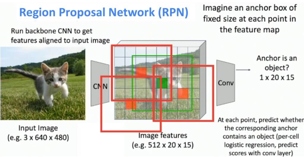
Region Proposal Network (RPN)
We will use an original input image and we will pass it through the backbone CNN. This will result in the desired feature map. We will introduce the so-called anchor boxes. This anchor box will be covering every element of the feature map. Some examples of anchor boxes are illustrated in the image below. Next, we will have a network that will tell us, using a simple binary classification, whether the anchor contains an object or not. In the image, green anchors are classified as regions with an object, whereas the red anchor boxes will be discarded from further analysis.
Furthermore, these anchor boxes may not fit perfectly to our object of interest. Therefore, another step to refine this anchor box is introduced. This refining process may be added to the PRN network that outputs four coordinates of the refined anchor box. Finally, this new bounding box will be called a proposal box.
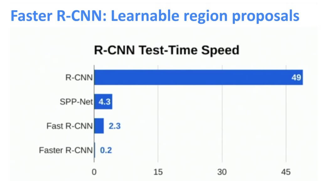
Hence, the overall algorithm is presented in the following diagram:

Finally, we have designed a network that is really really fast as compared with the original R-CNN. So, the effort to develop all the steps paid off indeed 🙂 The graph below represents the time needed to process a single image frame.
5. Faster R-CNN in PyTorch
In this part, we will just demonstrate how to use and apply the R-CNN network in PyTorch. Implementation from scratch would be too technical and full of details, so we will just take PyTorch’s built-in methods and models.
import torch
import numpy as np
import matplotlib.pyplot as plt

import torchvision.transforms.functional as F
In this step, we only use Torchvision’s tools for viewing images and creating bounding boxes.
plt.rcParams["savefig.bbox"] = 'tight'


def show(imgs):
    if not isinstance(imgs, list):
        imgs = [imgs]
    fig, axs = plt.subplots(ncols=len(imgs), squeeze=False)
    for i, img in enumerate(imgs):
        img = img.detach()
        img = F.to_pil_image(img)
        axs[0, i].imshow(np.asarray(img))
        axs[0, i].set(xticklabels=[], yticklabels=[], xticks=[], yticks=[])
We will download two images from the internet using the !wget command and we will create a grid of photos by using the make_grid() method. Images of dtype uint8 must be provided for this function.
!wget https://i.pinimg.com/736x/99/a6/fd/99a6fdcf4d023196d77eb36aa6082737--styles-php.jpg -O /content/car1.jpg
!wget https://i.pinimg.com/736x/dd/68/20/dd68208d216bb677bdab86579a856197--offroad-all-white.jpg -O /content/car2.jpg
from torchvision.utils import make_grid
from torchvision.io import read_image
from pathlib import Path
car1_int = read_image('car1.jpg')
car2_int = read_image('car2.jpg')
car_list = [car1_int, car2_int]
grid = make_grid(car_list)
show(grid)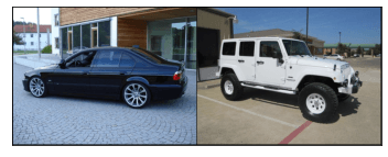
draw_bounding_boxes() can be used to draw boxes on an image. Colors, labels, width, font, and font size can all be customized. The boxes are formatted as (xmin, ymin, xmax, and ymax).
from torchvision.utils import draw_bounding_boxes

boxes = torch.tensor([[50, 50, 100, 200], [35, 120, 620, 390]], dtype=torch.float)
colors = ["blue", "yellow"]
result = draw_bounding_boxes(car1_int, boxes, colors=colors, width=5)
show(result)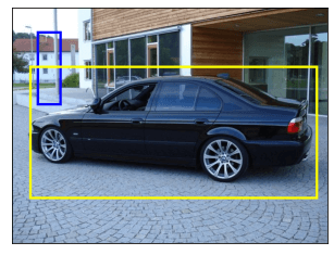
Of course, we can also depict the bounding boxes generated by models for torchvision detection. Here is a demonstration using the fasterrcnn_resnet50_fpn() model loaded with a Faster R-CNN model.
from torchvision.models.detection import fasterrcnn_resnet50_fpn, FasterRCNN_ResNet50_FPN_Weights

weights = FasterRCNN_ResNet50_FPN_Weights.DEFAULT
transforms = weights.transforms()

images = [transforms(d) for d in car_list]

model = fasterrcnn_resnet50_fpn(weights=weights, progress=False)
model = model.eval()

outputs = model(images)
print(outputs)
[{'boxes': tensor([[ 28.9595, 134.5368, 601.7979, 349.9137],
[193.5566, 140.5615, 265.0889, 167.9842],
[ 39.9696, 147.1586, 385.6311, 320.0778],
[ 56.1535, 57.3264, 70.2791, 74.9138],
[ 18.2229, 145.6895, 372.0598, 223.5003],
[306.9967, 138.4377, 609.1713, 338.3705],
[401.1234, 142.1768, 597.3285, 218.0435],
[194.6392, 136.0293, 311.0567, 178.4407],
[177.8387, 137.6242, 564.1535, 217.5274]], grad_fn=<StackBackward0>), 'labels': tensor([ 3, 3, 3, 10, 3, 3, 3, 3, 3]), 'scores': tensor([0.9975, 0.9756, 0.1578, 0.1235, 0.1173, 0.1015, 0.1010, 0.0596, 0.0592],
grad_fn=<IndexBackward0>)}, {'boxes': tensor([[ 50.2957, 92.2544, 559.3746, 394.2029],
[440.5210, 165.9631, 514.2350, 189.4745],
[ 1.0823, 66.7191, 80.6373, 216.8004],
[545.3552, 166.6906, 565.3425, 177.7227],
[623.8428, 166.1020, 639.8632, 175.8192],
[621.2831, 168.1364, 634.0815, 176.0556],
[630.9683, 166.2280, 640.0000, 174.9458],
[221.3280, 133.8347, 248.0095, 177.0258],
[544.7429, 167.2232, 556.0880, 176.6033],
[ 64.7255, 98.3926, 351.7974, 324.6750],
[ 0.0000, 62.4695, 107.9940, 258.9799],
[495.5164, 167.1042, 517.1301, 180.6814],
[441.0862, 167.3649, 456.5072, 175.7454],
[620.4214, 168.7013, 628.3602, 175.9150],
[ 5.8789, 11.4534, 196.9230, 289.0226],
[330.2793, 134.5042, 364.6375, 166.5594],
[544.6981, 166.3828, 566.0054, 178.1335],
[ 0.0000, 70.6256, 84.6627, 257.4922],
[554.5934, 167.3156, 566.4719, 177.3227]], grad_fn=<StackBackward0>), 'labels': tensor([ 8, 3, 72, 3, 3, 3, 3, 1, 3, 8, 8, 3, 3, 3, 8, 1, 8, 6,
3]), 'scores': tensor([0.9941, 0.9835, 0.9119, 0.9073, 0.8916, 0.5875, 0.5719, 0.2739, 0.1993,
0.1637, 0.1330, 0.1272, 0.1253, 0.0706, 0.0670, 0.0657, 0.0586, 0.0559,
0.0506], grad_fn=<IndexBackward0>)}]
Let’s visualize the boxes that our model found. Only boxes with scores higher than a specified threshold will be plotted.
score_threshold = 0.8
cars_with_boxes = [
    draw_bounding_boxes(dog_int, boxes=output['boxes'][output['scores'] > score_threshold], width=4)
    for dog_int, output in zip(car_list, outputs)
]
show(cars_with_boxes)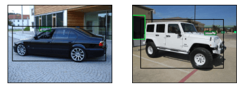
Summary
That would be all for this post. We have seen the theory behind the object detection algorithm R-CNN. We have seen the evolution of this algorithm and the next detection algorithms which are faster, Fast R-CNN and Faster R-CNN. In the end, we have written the code needed for running our own Faster R-CNN detector and detected cars on the images.
References
Michigan Online. (2020, August 10). Lecture 15: Object Detection [Video]. YouTube. https://www.youtube.com/watch?v=TB-fdISzpHQ