#004 Advanced Computer Vision - YOLO Object Detection

#004 Advanced Computer Vision – YOLO Object Detection

Highlights. Hello and welcome. In this post, we are going to talk about one of the most popular algorithms for object detection called the Yolo object detection algorithm.

We will cover the basic theory behind YOLO object detection [1], its benefits, and how this algorithm has evolved over the last couple of years. Finally, we will examine some real-life applications of YOLO object detection, more specifically, we will explain how to use YOLO for detecting basketball players on the court. So, let’s begin with our post.

Introduction to Object Detection

Object detection is a computer vision technique used for the identification and localization of objects within an image or a video. It is the process of identifying the correct location of one or multiple objects using bounding boxes, which correspond to rectangular shapes around the objects.

How does object detection work?

We can divide the process of object detection into 3 basic steps:

Image classification – answers the question “What is in this picture?”. It is a process of assigning an image to one of a number of different categories (e.g. car, dog, cat, human, etc.).
Object localization – answers the question “Where the object is in this picture?” This process allows us to find the exact location of our object in the image.
Object detection – provides the tools for object localization. This is done by drawing the so-called bounding boxes around objects.

Moreover, object detection algorithms can be divided into two groups.

Algorithms based on classification – select regions of interest in an image, and classify these regions using CNNs.
Algorithms based on regression – predict classes and bounding boxes for the whole image in one run of the algorithm. The best example that belongs to this group is the YOLO (You Only Look Once). This algorithm is commonly used for real-time object detection because it trades a bit of accuracy for large improvements in speed.

Now, let’s dive deeper into the theory behind the YOLO object detection algorithm.

What is YOLO?

You Only Look Once (YOLO) is a state-of-the-art, real-time object detection algorithm introduced in 2015 by Joseph Redmon, Santosh Divvala, Ross Girshick, and Ali Farhadi in their famous research paper “You Only Look Once: Unified, Real-Time Object Detection”. It is one of the most popular object detection algorithms because it uses one of the best neural network architectures to produce high accuracy and overall processing speed.

YOLO Architecture

Now, let’s examine the YOLO architecture in a little bit more detail. Let’s have a look at the following image.

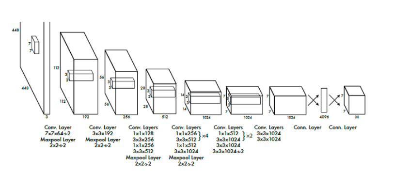
As you can see in the illustration above, this model has overall 24 convolutional layers, 4 max-pooling layers, and 2 fully connected layers. The input image is resized to the size of $448\times448 $ before going through the convolutional network. After that, $1\times1 $ convolution is applied to reduce the number of channels. This step is followed by a $3\times3 $ convolution. The activation function used in this model is ReLU, except for the final layer, which uses a linear activation function. Also note that some additional techniques, such as batch normalization and dropout, respectively regularize the model and prevent it from overfitting.

How Does YOLO Object Detection Work?

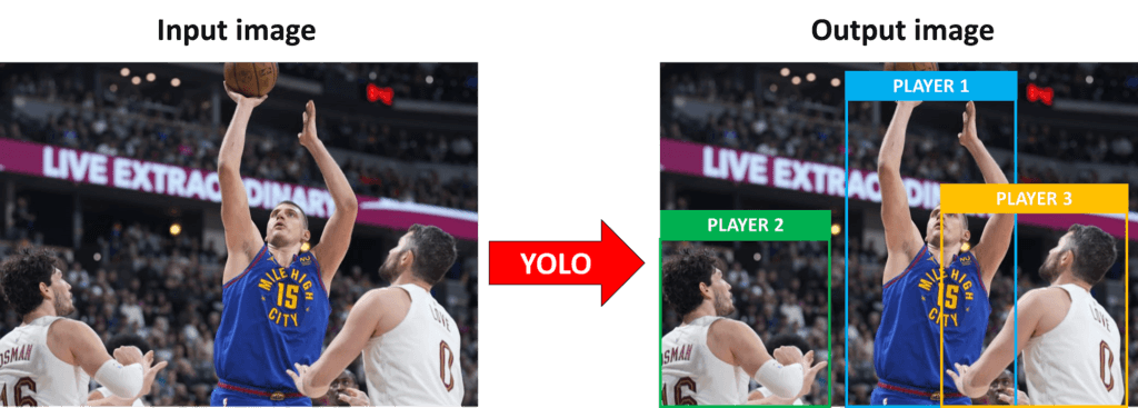
Now, let’s have a high-level overview of how object detection is performed with the YOLO algorithm. For that, we are going to use an example of basketball player detection. More specifically, we will explain how we can detect each basketball player on the court from a given input video.

To understand the whole process of object detection with the YOLO algorithm, our goal is to explain how we can get from an input image to an output image which is illustrated in the following example.

The algorithm works based on the following four steps:

Residual blocks
Bounding box regression
Intersection Over Unions or IOU
Non-Maximum Suppression.

Let’s have a closer look at each one of them.

1. Residual blocks

This first step is to divide the input image into $n \times n $ grid cells of equal shape. As you can see in the example below, in our case $n=4 $.

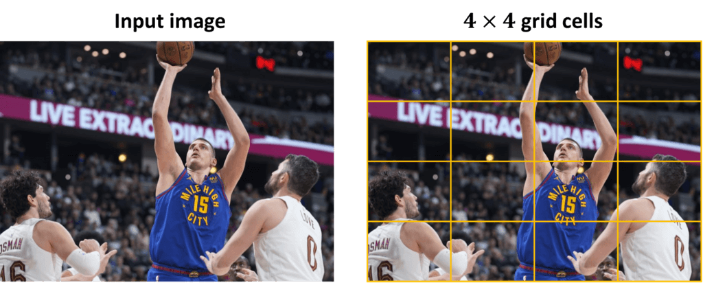
It is important to note that here, each cell in the grid is responsible for localizing and predicting the class of the object that it covers.

Bounding box regression

The next step is to determine the bounding boxes which correspond to rectangles highlighting all the objects in the image. We can have as many bounding boxes as there are objects within a given image.

YOLO determines the attributes of these bounding boxes using a single regression module where the vector the $Y $ is the final representation for each bounding box. Each vector is described with several parameters (numbers). The number of parameters depends on the number of objects in the image that we want to detect. The equation for the vector $Y $ can be written in the following way:

$$ Y=[p_{c}, b_{x}, b_{y}, b_{h}, b_{w}, c_{1}, c_{2}] $$

Let’s see what these parameters are :

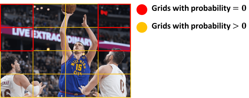
$p_{c} $ – corresponds to the probability score of the grid containing an object. For instance, in the image below we can see that all the grids in yellow will have a probability score higher than zero while the probability of each red cell will be equal to zero (insignificant).
$b_{x} $ and $b_{y} $, correspond to the $x $ and $y $ coordinates of the center of the bounding box.
$b_{w} $ and $b_{h} $, correspond to the height and the width of the bounding box.
$c_{1} $ and $c_{2} $, correspond to the two classes, which are in our case players and a ball. We can have as many classes as your use case requires.

To better understand these parameters, let’s take a look at the following image. We will isolate a player from the bottom left corner.

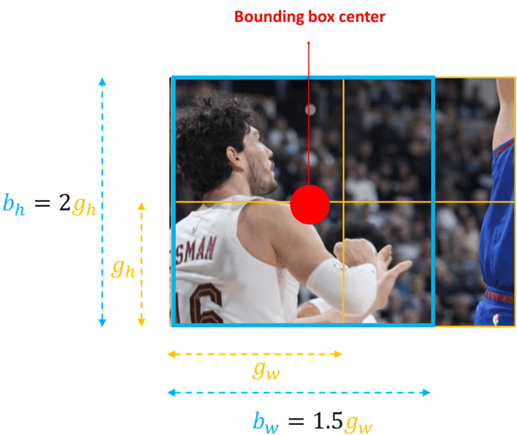
By looking at the image above we can see that parameter $b_{h} $ (bounding box height) is equal to $2g_{h} $(grid height) and $b_{w} $ (bounding box width) is equal to $1.5g_{w} $(grid width).

Intersection Over Unions (IOU)

Intersection over Union (IoU) is used to evaluate the performance of object detection by comparing the ground truth bounding box to the predicted bounding box. To better understand this topic check out this post.

Most of the time, a single object in an image will have multiple grid box candidates for prediction. However, usually, not all candidates are relevant. The goal of the IOU is to discard such grid boxes to only keep those that are relevant. This can be done in the following way:

The user defines its IOU selection threshold, for instance, 0.5.
The YOLO computes the IOU of each grid cell by calculating the intersection area divided by the union area.
The algorithm ignores the prediction of the grid cells having calculated IOU value below the threshold and considers those with an IOU above the threshold.

In the following image, we can see an illustration of applying the grid selection process to the bottom left object.

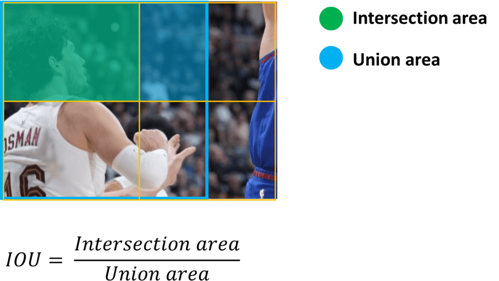
We can see that the object originally had two grid candidates. However, after applying the IOU method, only the second grid was selected.

Non-Max Suppression (NMS)

Setting a threshold for the IOU is not always enough because an object can have multiple boxes with IOU beyond the threshold, and leaving all those boxes might include noise. Here is where we can use NMS to keep only the boxes with the highest probability score of detection. To better understand this, let’s have a look at the following image.

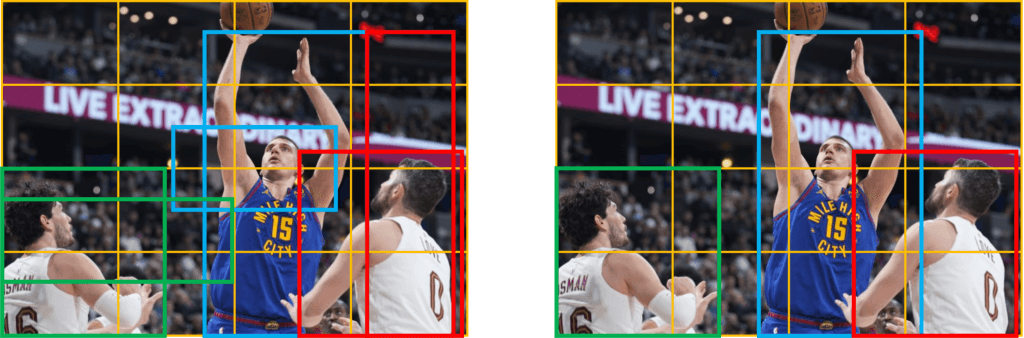
Notice that some of the bounding boxes can go outside the grid cell. Here we have two bounding boxes for each object. Our goal is to get rid of the bounding boxes with low probability $p_{c} $ and preserve only one bounding box with the highest probability.

Since the first release of YOLO in 2015, the algorithm has significantly evolved with different versions. Now, let’s understand the differences between each of these versions.

The evolution of the YOLO neural networks from v1 to v7

YOLOv1

The first version of YOLO, although it was a state-of-the-art algorithm for object detection at that time had several limitations:

Struggling to detect smaller images within a group of images, such as a group of persons in a stadium.
Unable to successfully detect new or unusual shapes.
The loss function used to approximate the detection performance treats errors the same for both small and large bounding boxes, which in fact creates incorrect localizations.

YOLOv2

YOLOv2 was created in 2016 with the idea of making the original YOLO model better and faster. The improvement includes the use of Darknet-19. It is a convolutional neural network that is used as the backbone of this version. Moreover, a new architecture, batch normalization, higher resolution of inputs, convolution layers with anchors, and dimensionality clustering was introduced in this version of YOLO.

YOLOv3

An incremental improvement has been performed on the YOLOv2 to create YOLOv3.

The changes for this version mainly include a new network architecture called Darknet-53. This is a faster, and much more accurate network compared to Darknet-19. This new architecture has been beneficial in many areas which are:

Better bounding box prediction
More accurate class predictions
More accurate prediction at different scales

YOLOv4

In the following image, we can see the comparison of the proposed YOLOv4 and other state-of-the-art object detectors.

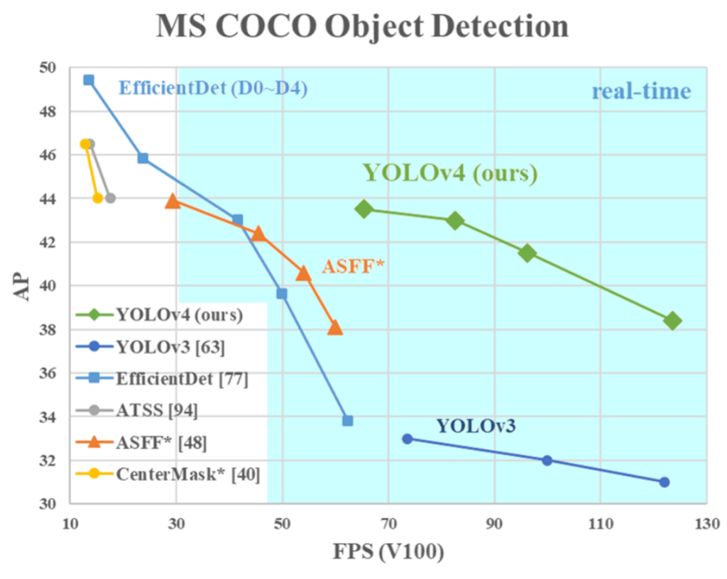
As you can see, YOLOv4 runs twice faster than EfficientDet with comparable performance. Furthermore, it improves YOLOv3’s average precision (AP) and FPS by 10% and 12%, respectively.

YOLOv5

YOLOv5, compared to other versions, does not have a published research paper, and it is the first version of YOLO that does not use the Darknet.

One of the major improvements of YOLOv5 architecture is the integration of the Focus layer. This is a single layer that is created by replacing the first three layers of YOLOv3. This integration reduced the number of layers, and a number of parameters and also increased both forward and backward speed without any major impact on the average precision.

YOLOv6

The YOLOv6 framework was released by a Chinese e-commerce company Meituan.

This new version was not part of the official YOLO but still got the name YOLOv6 because its backbone was inspired by the original one-stage YOLO architecture.

YOLOv6 introduced three significant improvements to the previous YOLOv5: a hardware-friendly backbone and neck design, an efficient decoupled head, and a more effective training strategy.

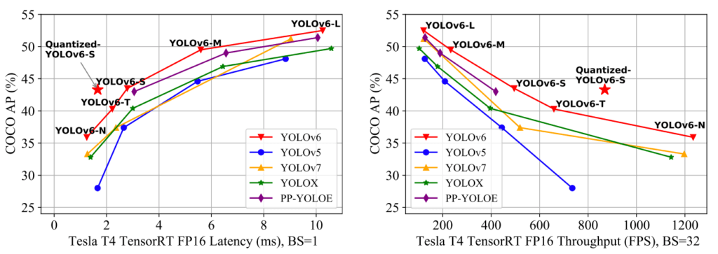
YOLOv6 is written in Pytorch and provides outstanding results compared to the previous YOLO versions in terms of accuracy and speed on the COCO dataset as illustrated in the image below.

YOLOv7

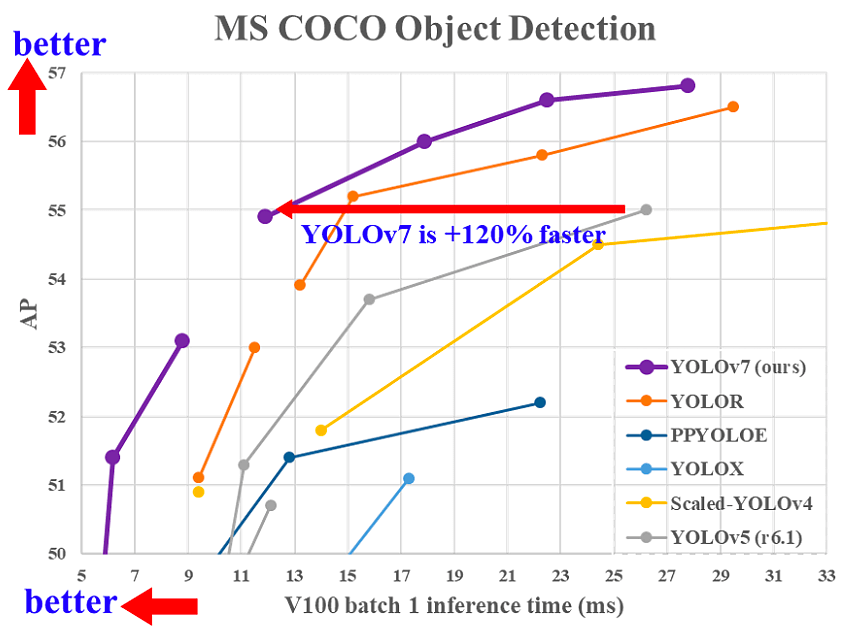
YOLOv7 was released in July 2022 in the paper “Trained bag-of-freebies sets new state-of-the-art for real-time object detectors”. This version is making a significant move in the field of object detection, and it surpassed all the previous models in terms of accuracy and speed as you can see in the following image.

YOLOv7 significantly reformed its architecture by integrating the Extended Efficient Layer Aggregation Network (E-ELAN). This network allows the model to learn more diverse features for better learning.

YOLOv8

YOLOv8 is developed by Ultralytics, and it is a cutting-edge, state-of-the-art model that builds upon the success of previous YOLO versions and introduces new features and improvements to further boost performance and flexibility. YOLOv8 is designed to be fast, accurate, and easy to use, making it an excellent choice for a wide range of object detection, image segmentation, and image classification tasks.

Now that we have learned the theory behind the YOLO algorithm and explored all versions that have been released, we can move on to the one practical task. Let’s see how we can run the YOLOv7 algorithm in Python [2].

YOLOv7 in Python

In order to speed up object detection with YOLOv7, we need to change runtime settings in Google Colab and enable the GPU option.

The next step is to connect our google drive with Google Colab. To do that we will import drive and use the following command.

from google.colab import drive
drive.mount('/content/gdrive')Code language: JavaScript (javascript)

Now, we need to move to Google drive and we can do that with the following command.

%cd /content/gdrive/MyDrive/

Then we will create a folder called TheCodingBug where we will clone the YOLOv7 repository.

import os

if not os.path.isdir("TheCodingBug"):
  os.makedirs("TheCodingBug")Code language: JavaScript (javascript)

Now, we can move to this newly created directory and clone the YOLOv7. To do that you just go to the official YOLOv7 git page and copy the code link.

%cd TheCodingBug

! git clone https://github.com/WongKinYiu/yolov7.gitCode language: PHP (php)

After cloning the repository, we want to download the pre-trained model that we want to run for object detection. To do that we just need to copy the link from the official YOLOv7 GitHub page.

!wget https://github.com/WongKinYiu/yolov7/releases/download/v0.1/yolov7.ptCode language: JavaScript (javascript)

Next, we need to upload the video that we want to use to the folder TheCodingBug . Finally, we can use the following command to run object detection with YOLOv7. Let’s see our results.

!python detect.py --weights yolov7.pt --conf 0.5 --img-size 640 --source leBron.mp4Code language: CSS (css)

As you can see, each player on the court is successfully detected. Above the bounding box around the players, we can also see the confidence score. The algorithm also detects the people in the crowd. In some future posts, we will cover the topic of how to avoid detection of the undesirable objects.

Summary

In this post, we learned how to perform object detection using one of the most popular and accurate object detection algorithms called YOLO. We explained the basic idea of YOLO object detection. We also took a deeper look into the evolution and current applications of the YOLO algorithm. Moreover, we have seen how we can run the YOLOv7 algorithm with Python in Google Colab.

References:

[1] YOLO Object Detection Explained

[2] Official YOLO v7 Object Detection COMPLETE Tutorial for Google Colab

#004 Advanced Computer Vision – YOLO Object Detection