Highlights: Yu Su’s guest lecture in the UC Berkeley CS294-280 course argues language agents are not “LLM + tools” but a new evolutionary stage of machine intelligence. We walk through the agent-first framing and three concrete research pillars — long-term memory (HippoRAG), implicit reasoning (Grokked Transformers), and model-based planning (WebDreamer) — that map directly to classical AI problems re-examined through the lens of LLMs.

• Agent-first framing: token generation is itself an action; the inner monologue is a literal reasoning loop, not a metaphor
• HippoRAG: hippocampal indexing theory → schema-free knowledge graph + personalized PageRank → +7.3 Recall@5 over dense retrieval, +8.2 over IRCoT on multi-hop QA
• Grokked Transformers: implicit reasoning emerges only through grokking; data distribution (ratio \(\phi\)) drives generalization, not data size
• Circuit analysis: composition forms a staged circuit, comparison forms a parallel circuit — circuit shape determines OOD systematicity
• WebDreamer: use the LLM itself as a transition model \(\hat{T}: S \times A \to S\) to simulate before committing — solves the irreversibility problem of tree search on real websites
• Deep reasoning result: on a hard multi-hop task with no surface clues, a grokked transformer hits near-perfect accuracy while o1-preview + RAG fails badly — parametric memory wins when the search space is vast

Tutorial Overview:

1. Redefining agents for the LLM era
2. Long-term memory — HippoRAG
3. Implicit reasoning — Grokked Transformers
4. Model-based planning — WebDreamer
5. The road ahead and open challenges
6. Appendix — parametric vs. non-parametric memory for deep reasoning

---

1. Redefining Agents for the LLM Era

1.1 Two views of what an agent is

The discourse around agents is split. Bill Gates calls them the biggest shift since the GUI. Andrew Ng predicts agentic workflows will drive the next wave of AI progress. Sam Altman declared 2025 the year agents will actually work. On the other side, critics dismiss current systems as glorified LLM wrappers and point to AutoGPT — once one of the fastest-growing GitHub repos ever — as a cautionary tale of hype outrunning capability.

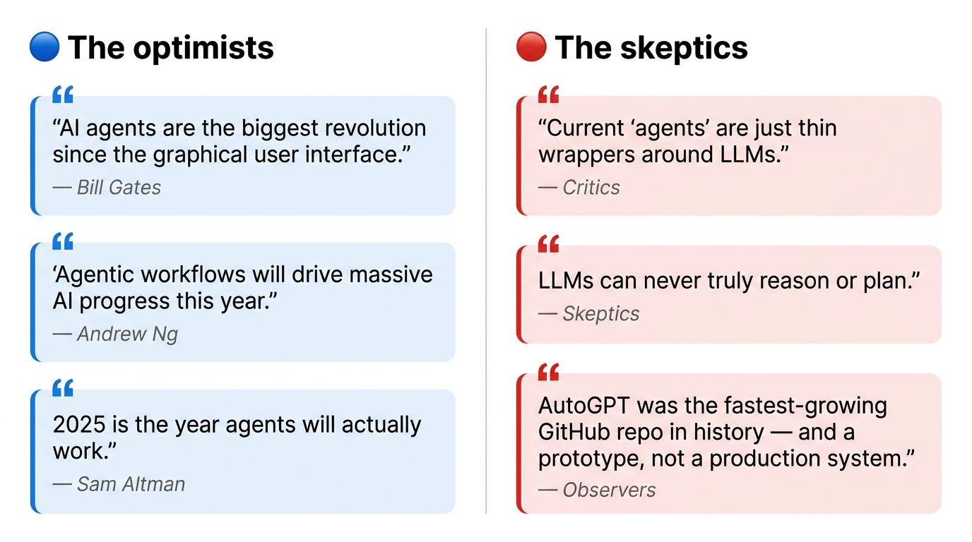
Fig 1. The divide: optimistic predictions about AI agents on one side, critical concerns about hype and capability on the other.

But agents are not new. The Russell & Norvig definition from any AI 101 textbook — “an agent is anything that can be viewed as perceiving its environment through sensors and acting upon that environment through actuators” — has been around for decades. The perception-action loop is the foundational pursuit of AI. The interesting question is not “are agents new” but “what changed.”

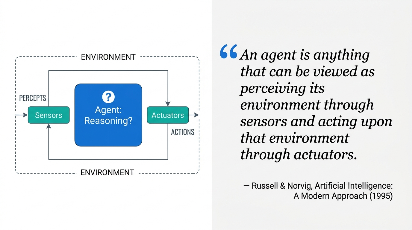
Fig 2. The classic agent architecture — perception-action cycle. Sensors feed an internal decision module; actuators act on the environment.

The standard answer: we now hook an LLM up to an external environment. The model perceives information from the world and acts upon it, instead of doing text-in, text-out.

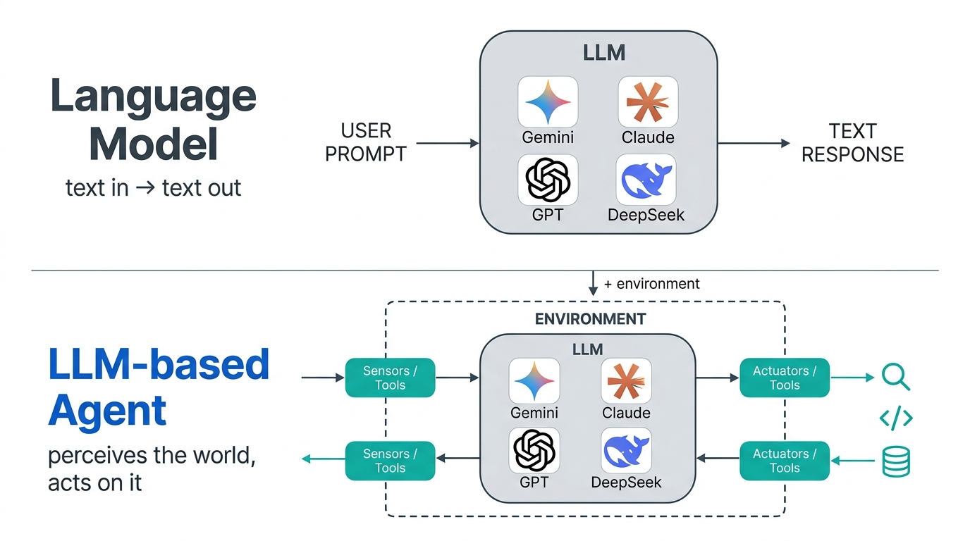
Fig 3. From language models to LLM-based agents. The model gains an interface to the world.

This framing is incomplete. Self-reflection — the LLM examining its own reasoning trace and changing course — has no clean place in a sensor/actuator diagram. Neither do multi-agent simulations, where multiple LLMs interact mostly with each other, not with anything we’d call an environment. Something deeper is going on than “LLM with API calls.”

1.2 LLM-first vs. agent-first

The community is split between two perspectives, and the distinction matters more than it sounds.

The LLM-first view starts from the model. We have powerful LLMs that know vast amounts of information — let’s scaffold them into agents. The natural mode of work is prompt engineering, tool wrappers, framework design. This is exactly the perspective that produces the “agents are just glorified wrappers” critique — because in this framing, that critique is essentially correct.

The agent-first view inverts this. AI agents have been the central pursuit of the field since its inception. They did not appear with ChatGPT. What changed is that we can now plug LLMs into traditional agent architectures, giving them a new capability: using language as the medium for reasoning and communication.

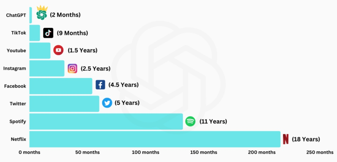
Fig 4. ChatGPT reached 100 million users in just 2 months — faster than any previous platform.

This distinction changes which problems you focus on. The LLM-first view points at prompts and APIs. The agent-first view points back at the classical hard problems of AI — perception, reasoning, world models, planning — and asks how language models reshape each one. It also opens up new opportunities: synthetic data generation at scale, self-reflection loops, internalized search of the kind that powers o1-style reasoning models.

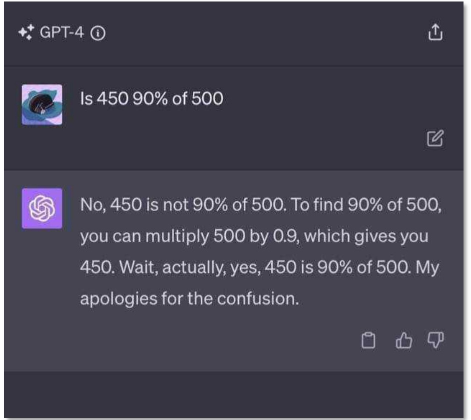
Fig 5. GPT-4 demonstrating self-correction on a mathematical reasoning task — a capability that does not fit the classical sensor/actuator model.

Key idea: The agent-first framing recontextualizes the LLM as one transformative component within a broader agent architecture, rather than treating the agent as an accessory to the language model. The classical challenges — perception, reasoning, world models, planning — remain. They just look different through the lens of LLMs.

1.3 Token generation as action

The conceptual move that does the most work: token generation itself is a form of action. Not just a way to produce output, but a mechanism for taking actions inside an internal environment.

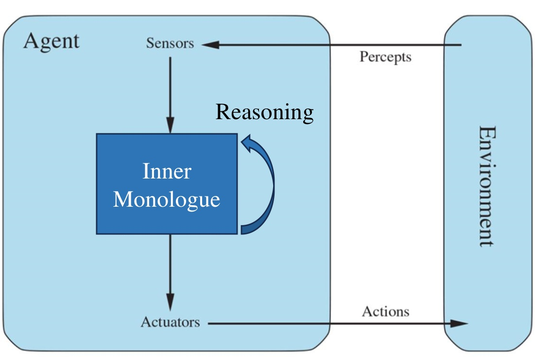
Fig 6. Language agent architecture. Sensors feed an inner-monologue reasoning loop, which drives both internal state updates and external actuators.

Once you accept this, things fall into place. Self-reflection becomes a meta-reasoning action — the agent acting on its own reasoning trace, much like metacognition in humans. The inner monologue is not a metaphor. It is a literal loop where token generation operates on previously generated tokens. And crucially, reasoning is for better acting: the inner monologue exists to infer environmental states, replan, and make external behaviour more effective.

Unlike traditional ML systems that commit a fixed amount of compute per decision, LLMs adaptively allocate compute by generating more tokens. This is what gives them the “second chance to think” that makes chain-of-thought work at all.

1.4 Why call it “reasoning”?

The term reasoning is overloaded. There is a principled justification for it. In Daniel Kahneman’s dual-process framework, human cognition breaks down into perception (what is there), intuitive inference (fast, effortless pattern matching), and symbolic reasoning (slow, effortful deliberation) — with separate cognitive subsystems for each.

Fig 7. A scene that demands perception, intuitive inference, and contextual reasoning all at once.

LLMs have one mechanism — token generation — for all of this. GPT-4o’s response to the kitchen scene blends perception (“a young boy sitting on the floor”), intuitive inference (“appears to be sad or remorseful”), and complex reasoning about social dynamics (“her body language suggests she is asking him what happened”). All three happen in the same forward pass.

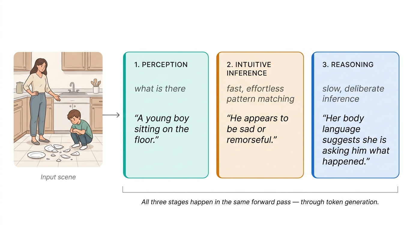
Fig 8. GPT-4o’s response factored into Perception → Intuitive Inference → Reasoning. All three stages happen through the same token generation mechanism.

Unlike humans, where perception is effortless and reasoning is effortful, everything is effortful for LLMs — every stage requires explicit token generation. That unified mechanism is exactly why “reasoning” works as a generalized term for the whole process.

1.5 Language agents as a new evolutionary stage

Human cognition takes raw multimodal sensory input and fuses it into a unified neural representation that both reconstructs the world and supports symbolic reasoning. Earlier AI systems could only approximate this in narrow, fragmented ways.

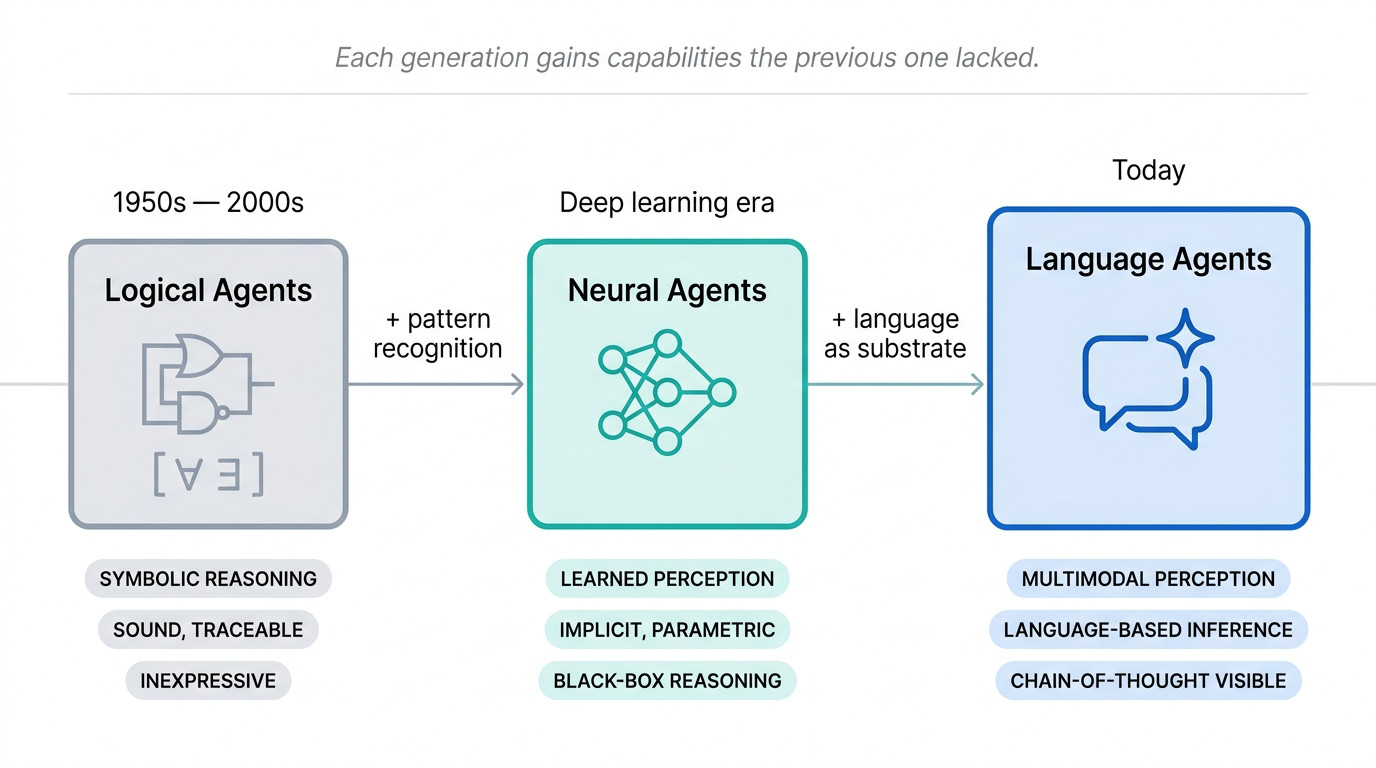
Fig 9. The progression from logical agents to neural agents to language agents — increasing expressiveness, reasoning ability, and adaptivity.

Logical agents captured symbolic reasoning. Neural agents captured perceptual pattern recognition. Neither captured both. Multimodal LLMs and the language agents built on them are the first systems where multi-sensory inputs land in a unified neural representation that is also conducive to symbolic reasoning and communication. Three dimensions improve dramatically compared to prior agent paradigms: expressiveness, reasoning visibility, and adaptivity.

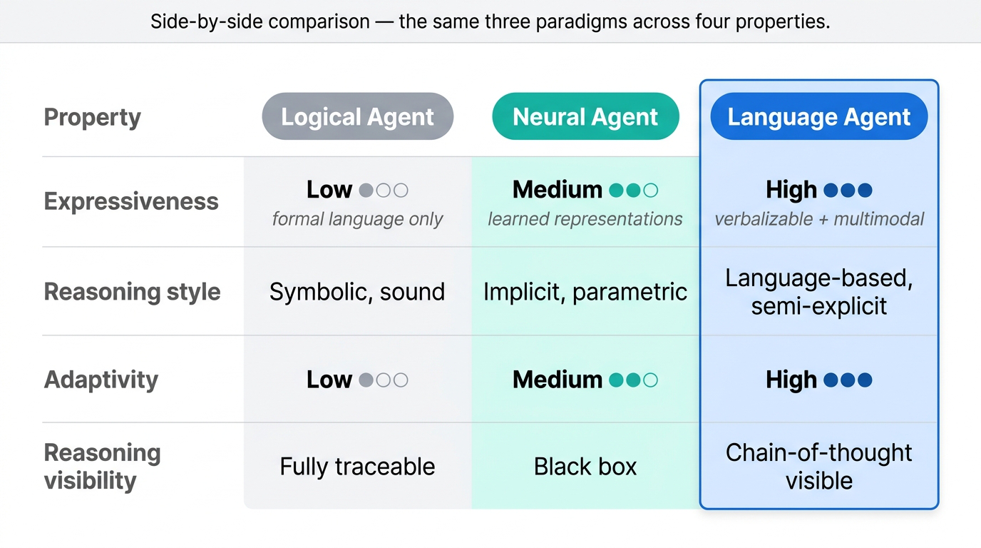
Fig 10. Side-by-side comparison of logical, neural, and language agents.

Property	Logical Agent	Neural Agent	Language Agent
Expressiveness	Low (formal language)	Medium (learned)	High (verbalizable + multimodal)
Reasoning style	Symbolic, sound	Implicit, parametric	Language-based, semi-explicit
Adaptivity	Low	Medium	High
Reasoning visibility	Fully traceable	Black box	Chain-of-thought visible

Logical agents had high precision but their formal languages put a hard ceiling on expressiveness. Neural agents got medium expressiveness through learned representations, but their reasoning was purely parametric and opaque. Language agents hit high expressiveness because they can encode anything verbalizable, plus the non-verbalizable through multimodal perception.

The reasoning style is the most interesting axis. Language agents perform language-based inference — fuzzy, flexible, semi-explicit. You can read the chain of thought as it unfolds, which you cannot do with the parametric reasoning of a pure neural net. The fuzziness is not a bug. The world is fuzzy. Rigid logical systems pay for soundness with a massive sacrifice in expressiveness.

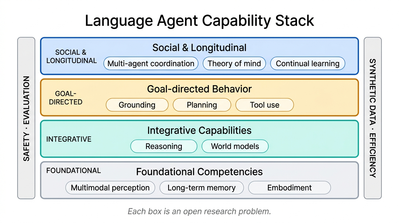
Fig 11. The conceptual framework for language agents. Foundational competencies at the base, integrative capabilities in the middle, social and longitudinal capabilities at the top. Cross-cutting concerns span the entire stack.

This framework is a research roadmap, not just a taxonomy. At the base sit multimodal perception, memory, and embodiment. The middle layer adds reasoning and world models. Above that come grounding, planning, and tool use. At the top: multi-agent coordination, theory of mind, continual learning. Cross-cutting: safety, evaluation, synthetic data, efficiency.

The rest of this post drills into three boxes: memory (HippoRAG), reasoning (Grokked Transformers), and planning (WebDreamer).

---

2. Long-Term Memory — HippoRAG

2.1 Why current RAG falls short on multi-hop queries

Standard RAG has become the default way to give LLMs access to external knowledge. When ChatGPT does not know who won the 2024 Super Bowl, it retrieves and grounds. This sidesteps catastrophic forgetting elegantly: instead of constantly retraining parameters, store new experiences outside the model and pull them in on demand.

RAG only works if the LLM is actually receptive to retrieved evidence. A paper from Yu Su’s group at Ohio State University, “Adaptive Chameleon or Stubborn Sloth”, studies what happens when retrieved context conflicts with the model’s parametric memory. Finding: LLMs are highly receptive to external evidence, even when it contradicts their internal knowledge, as long as that evidence is coherent and convincing. Good news for RAG. Concerning news for safety, since susceptibility to convincing external evidence cuts both ways.

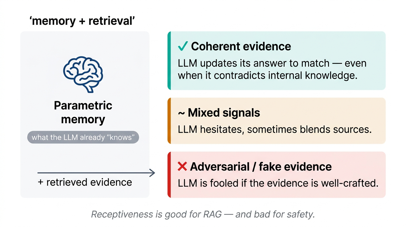
Fig 12. LLM behavior under knowledge conflicts. Coherent external evidence overrides parametric memory.

The foundation is solid. The problem is that today’s RAG is far less sophisticated than human memory. The standard pipeline embeds passages into vectors and retrieves on cosine similarity to the query embedding. That flat token-level matching breaks badly on queries that require multi-hop reasoning across documents.

Concrete example: “Which Stanford professor works on Alzheimer’s?” Suppose the knowledge base has separate passages — one saying “Thomas works at Stanford” and another saying “Thomas studies Alzheimer’s neuroscience” — but no single passage that connects both facts.

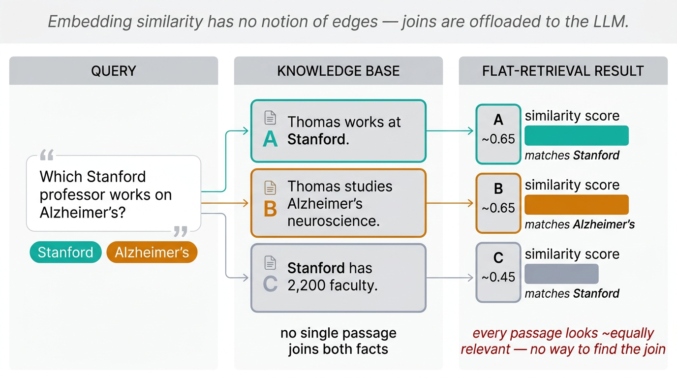
Fig 13. The multi-hop failure mode. Each passage covers only half the query, so all candidates score equally relevant.

When you embed each passage and compare to the query, every passage looks equally relevant — each captures roughly half the query’s semantic content. You retrieve a pile of “Stanford professors” passages and a pile of “Alzheimer’s researchers” passages, with no efficient way to find the one person at the intersection. The LLM is stuck sifting through thousands of passages looking for a name that satisfies both constraints.

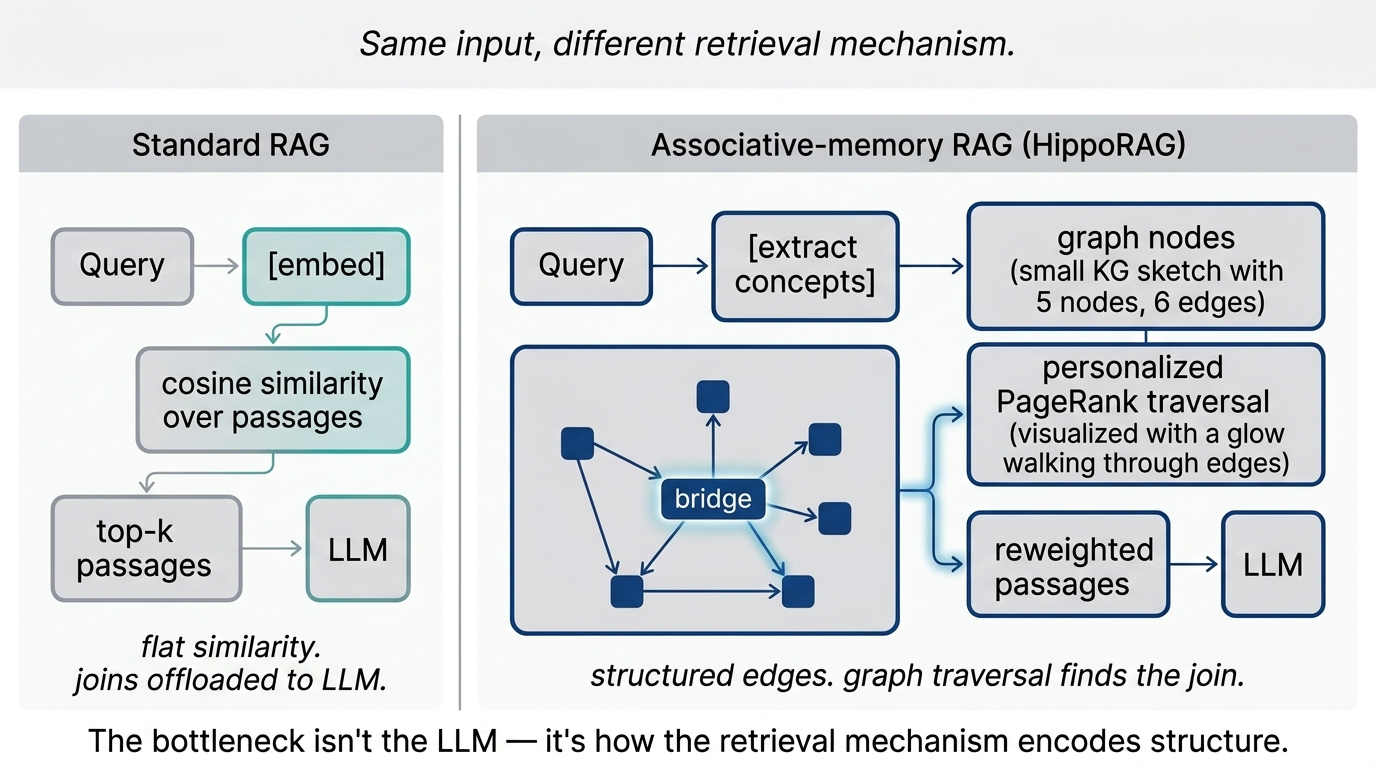
Fig 14. Standard RAG vs. an associative memory approach. The retrieval mechanism — flat similarity vs. graph traversal — is the bottleneck.

Key idea: Human memory builds associations between facts. When you encounter “Thomas works at Stanford” and “Thomas works on Alzheimer’s” separately, your brain builds a link. Embedding-based RAG has no equivalent — it stores points in a vector space, not edges between concepts.

2.2 Hippocampal indexing — the biological blueprint

The hippocampus does not store memories. It stores indices that point to memories distributed across the neocortex. This is the core insight of hippocampal indexing theory (Teyler et al., 1986), one of the most well-established models of human long-term memory.

Fig 15. The hippocampus (blue) sits in the medial temporal lobe and serves as the index for memories distributed across the neocortex.

When you experience something — a conversation at a coffee shop — different aspects are stored where they were first processed. Visual details in the visual cortex, sounds in the auditory cortex. The hippocampus maintains a structured index that binds those distributed fragments together through associations. That is why recalling a memory feels like reliving it: you are reactivating the same neural patterns that fired during the original experience.

This indexing architecture enables two capabilities that flat embedding RAG fundamentally cannot:

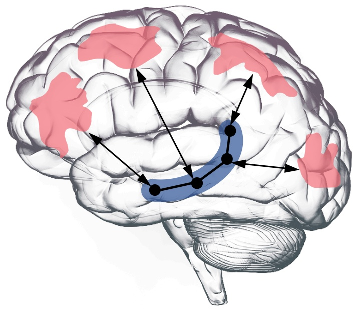
Fig 16. Neocortex (pink/red) and hippocampus (blue) jointly enable pattern separation and pattern completion.

• Pattern separation — differentiating extremely similar memories at fine granularity. Two consecutive seconds of your day are nearly identical, yet you can distinguish them. Operates at the conceptual level through the interplay between neocortex and parahippocampal regions, far beyond what raw vector similarity captures.
• Pattern completion — recovering a complete memory from partial cues. When you hear “Stanford” and “Ishmael,” the CA3 region of your hippocampus reconstructs the full associative network connecting that person to both institutions.

2.3 HippoRAG architecture

HippoRAG maps three brain regions involved in long-term memory directly to computational components.

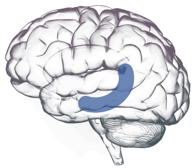
Fig 17. The hippocampus (blue) within the medial temporal lobe — provides indexing and auto-associative recall.

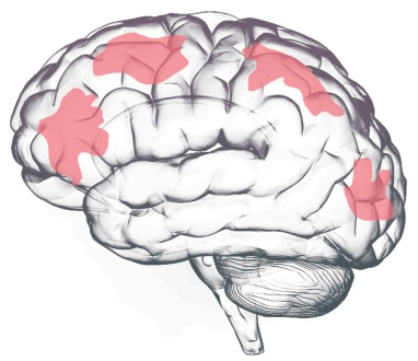
Fig 18. Neocortex regions (pink/red) across the cerebral cortex — handles perception, language, and reasoning.

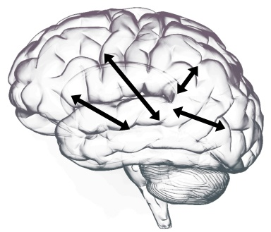
Fig 19. Parahippocampal region with connectivity pathways — bridge between neocortex and the hippocampal index.

Brain region	Function	HippoRAG component
Neocortex	Perception, language, reasoning	LLM (open information extraction)
Parahippocampal regions	Bridge, working memory	Dense retrieval encoder
Hippocampus	Indexing, auto-associative recall	Schema-free KG + personalized PageRank

The system runs in two phases.

Offline indexing. An LLM acts as the neocortical component, performing open information extraction on input passages to pull out triplets — concepts (noun phrases) and their relationships (verb phrases). These become nodes and edges in a knowledge graph that serves as the hippocampal index. Importantly, this is a schema-free knowledge graph with no predefined ontology. Everything emerges from the LLM’s processing of raw text.

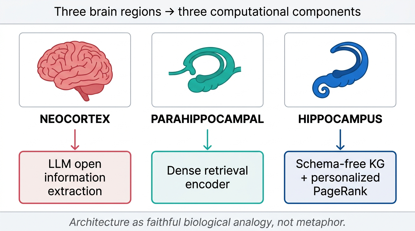
Fig 20. HippoRAG architecture — three components mapped to three brain regions.

The parahippocampal encoder uses retrieval models to consolidate information, identifying which concepts are similar or synonymous. It bridges the pattern-separated concepts from the neocortex and the structured hippocampal index.

Online retrieval. When a query arrives — like the Stanford-Alzheimer’s example — the system uses NER to identify key concepts. A dense retriever finds similar nodes in the hippocampal index, which become seed nodes for graph traversal. Then it runs personalized PageRank, a random walk that starts from seed nodes and disperses probability mass to neighbours.

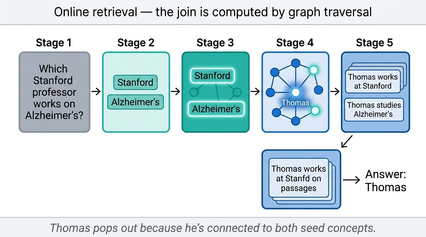
Fig 21. End-to-end view — offline indexing on top, online retrieval below.

Nodes close to multiple seed nodes accumulate higher weight. In the Stanford example, Professor Thomas — connected to both “Stanford” and “Alzheimer’s” — surfaces with the highest weight. Concept weights then reweight the original passages, surfacing the most relevant content.

2.4 Results and the v2 update

HippoRAG delivers strong results on multi-hop QA. On average it outperforms the best single-step dense retrieval baseline by +7.3 points in Recall@5. When combined with the multi-step IRCoT method, the integrated approach beats IRCoT alone by +8.2 points. The complementarity is the key — because HippoRAG is fundamentally a structured index with graph search, it slots into existing retrieval pipelines for substantial gains.

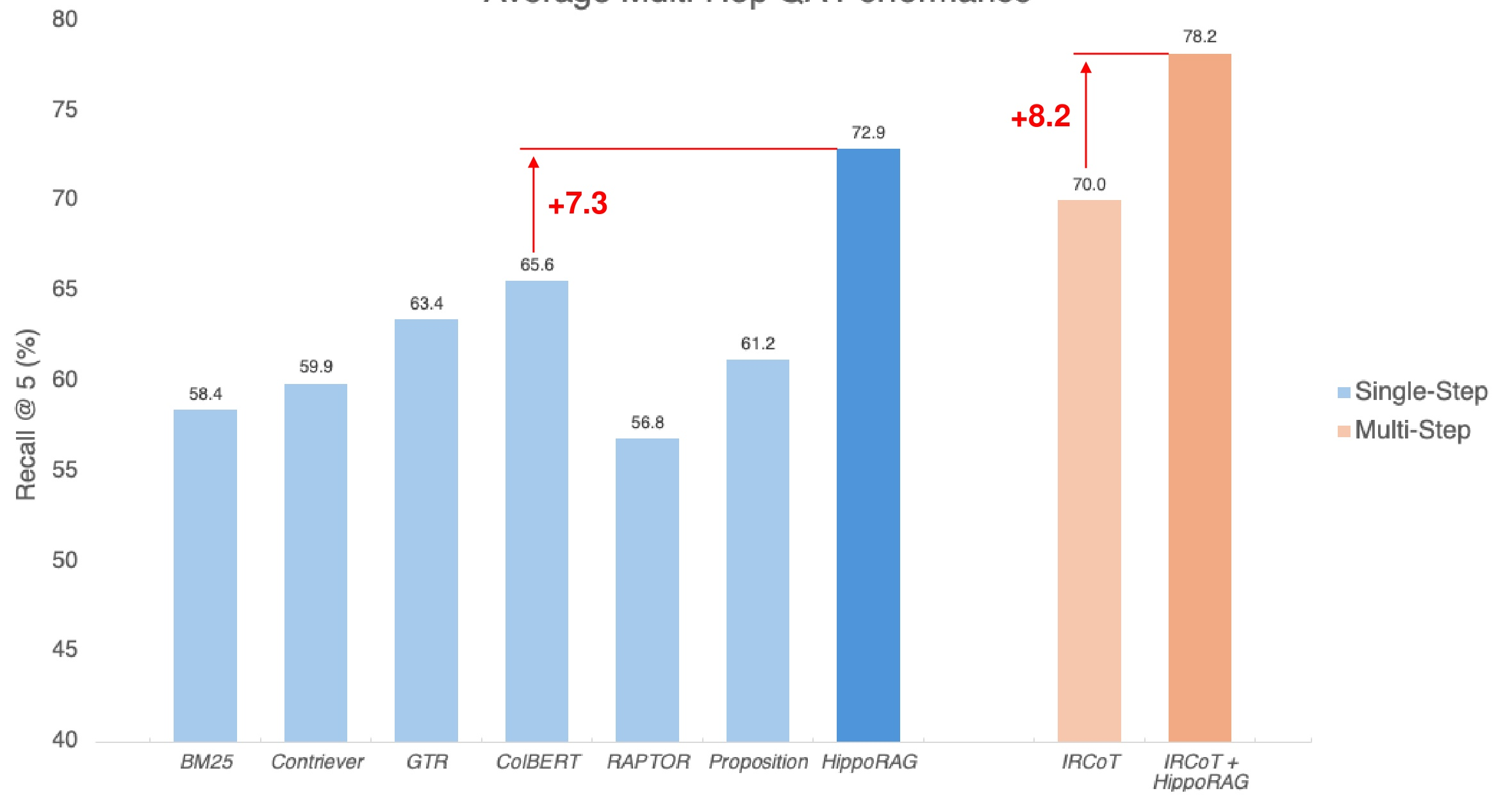
Fig 22. HippoRAG vs. single-step and multi-step baselines on multi-hop QA. Recall@5 across HotpotQA, 2WikiMultihopQA, and MuSiQue.

The gains show up most clearly on path-finding questions — queries that require traversing complex relational structures. Take the running example: “Which Stanford professor works on Alzheimer’s neuroscience?” The solution path is not a one-hop lookup. It starts with a one-to-many relation (Stanford → many professors), then narrows through a many-to-one relation (many researchers → Alzheimer’s). Without prior knowledge of the answer, a flat retriever has to search through hundreds or thousands of candidates.

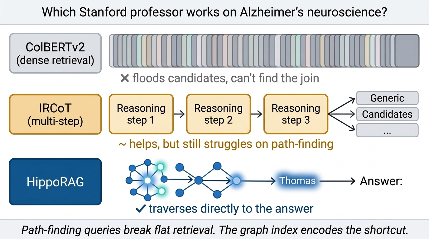
Fig 23. HippoRAG vs. ColBERTv2 and IRCoT on path-finding questions. Only HippoRAG navigates the multi-hop path efficiently.

HippoRAG explicitly extracts and indexes these associations from raw text, building shortcuts that let it traverse efficiently to the right answer. Dense retrievers like ColBERTv2 — and even iterative methods like IRCoT — struggle on these multi-hop paths.

There is a catch worth flagging. While HippoRAG and other structure-augmented RAG methods (GraphRAG, LightRAG, RAPTOR) do well on multi-hop QA, they often underperform large embedding models like voyage or mxbai-embed on simpler single-hop QA or discourse understanding tasks. That has historically made structured approaches hard to adopt as a drop-in replacement.

HippoRAG v2 closes that gap. With a series of refinements, v2 lands at performance comparable to or better than the best large embedding models across the board — not just on multi-hop QA but also on simple QA and narrative understanding. That makes it far more practical as a general-purpose retrieval backbone.

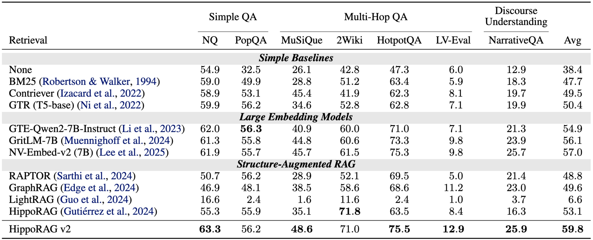
Fig 24. HippoRAG v2 across diverse QA benchmarks — competitive with or better than the best large embedding models.

Key idea: The earlier “good at multi-hop, mediocre at single-hop” trade-off was a deal-breaker for general-purpose use. HippoRAG v2 makes the structured-index approach a viable drop-in for production memory systems.

---

3. Implicit Reasoning — Grokked Transformers

3.1 Why implicit reasoning matters even in the chain-of-thought era

The conversation shifts from memory to reasoning — specifically, the kind that happens inside the forward pass with no explicit chain of thought. The relevant work is a paper from Yu Su’s group at Ohio State University, Grokking of Implicit Relations in Transformers, which takes a mechanistic look at how transformers acquire structured reasoning during pretraining.

Implicit reasoning means the model predicts an answer directly in a single forward pass, with no verbalized intermediate steps. Toy example: if the model has memorized that GPT-4’s creator is OpenAI, and that OpenAI’s CEO is Sam Altman, can it answer “GPT-4 [creator] [CEO] = ___” with “Sam Altman” without writing out the intermediate steps?

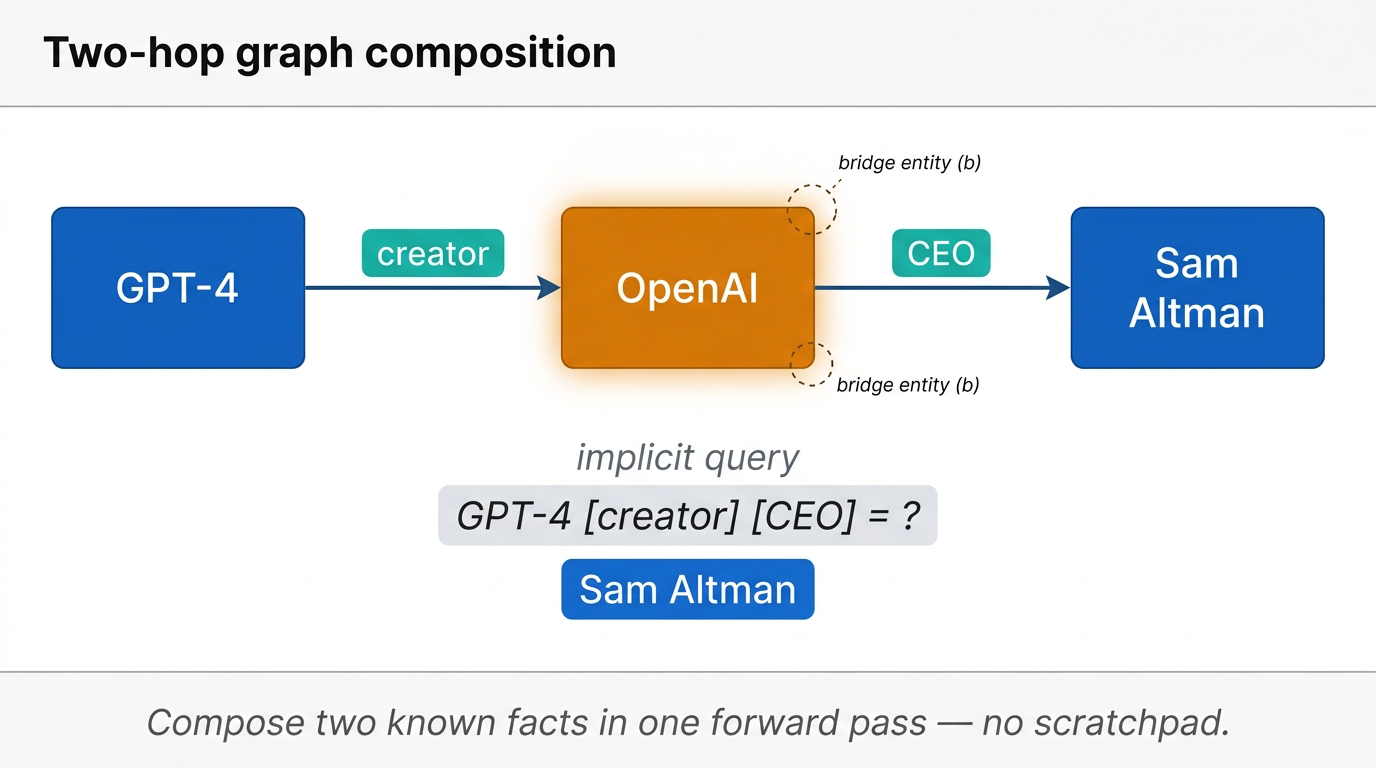
Fig 25. Two-hop graph composition — GPT-4 → creator → OpenAI → CEO → Sam Altman. The bridge entity (OpenAI) must be inferred internally.

Given the dominance of long chain-of-thought reasoning right now — o1, R1, all the rest — why care about implicit reasoning?

1. Implicit reasoning is the default mode of pretraining. Standard next-token prediction with cross-entropy loss has no chain of thought. The model has to compress the data and reason implicitly just to predict the next token reasonably well. Any post-training story sits on top of this baseline.
2. It determines how well LLMs acquire structured representations of facts and rules from training data. If the model cannot learn to compose or compare facts during pretraining, no amount of clever prompting will fully recover that.
3. It may be the substrate o1-style reasoning is built on. The hypothesis: a capable base model has already learned a library of basic reasoning constructs in implicit form. RL then incentivizes the right combinations of these strategies, rather than learning entirely new reasoning primitives from scratch.

3.2 The documented struggles

Until this work, the literature was pessimistic. Multiple studies showed LLMs failing at implicit reasoning:

• Composition — models showed substantial evidence only for first-hop reasoning, and the “compositionality gap” did not shrink with scale (Press et al. 2023; Yang et al. 2024).
• Comparison — even GPT-4 struggled to implicitly compare entity attributes — for example, determining which of GPT-4 (released March 2023) or Claude 3 (released March 2024) is newer, despite knowing each model’s release date individually (Zhu et al. 2023).

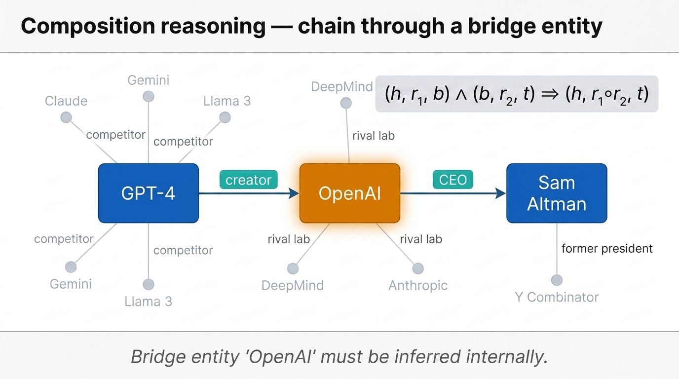
Fig 26. Composition reasoning — GPT-4 → creator → OpenAI → CEO → Sam Altman, embedded in a broader AI-company knowledge graph. The bridge entity OpenAI must be inferred without a scratchpad.

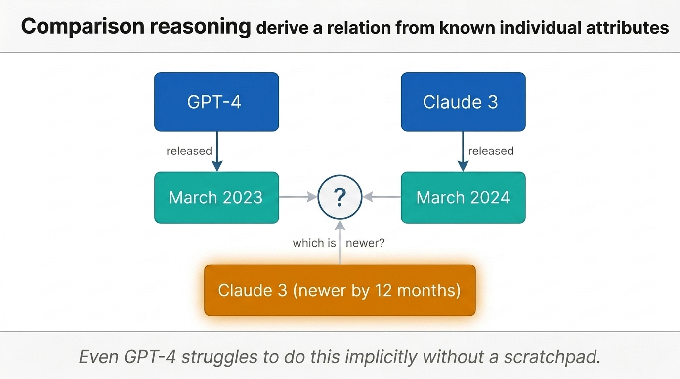
Fig 27. Comparison reasoning — GPT-4 (March 2023) vs. Claude 3 (March 2024). Implicit comparison should derive “which is newer” from individually known release dates, without intermediate steps.

These results fed the broader narrative that autoregressive LLMs “never truly reason or plan.” Yu Su’s group bet the truth was more nuanced.

3.3 Experimental setup — random knowledge graphs

To study compositional reasoning and deduction rules in isolation, the team built a controlled environment using synthetic random knowledge graphs. The architecture is deliberately standard: a decoder-only transformer in the GPT-2 mold — 8 layers, 768 hidden dimensions, 12 attention heads. AdamW, learning rate \(1\mathrm{e}{-4}\), batch size 512.

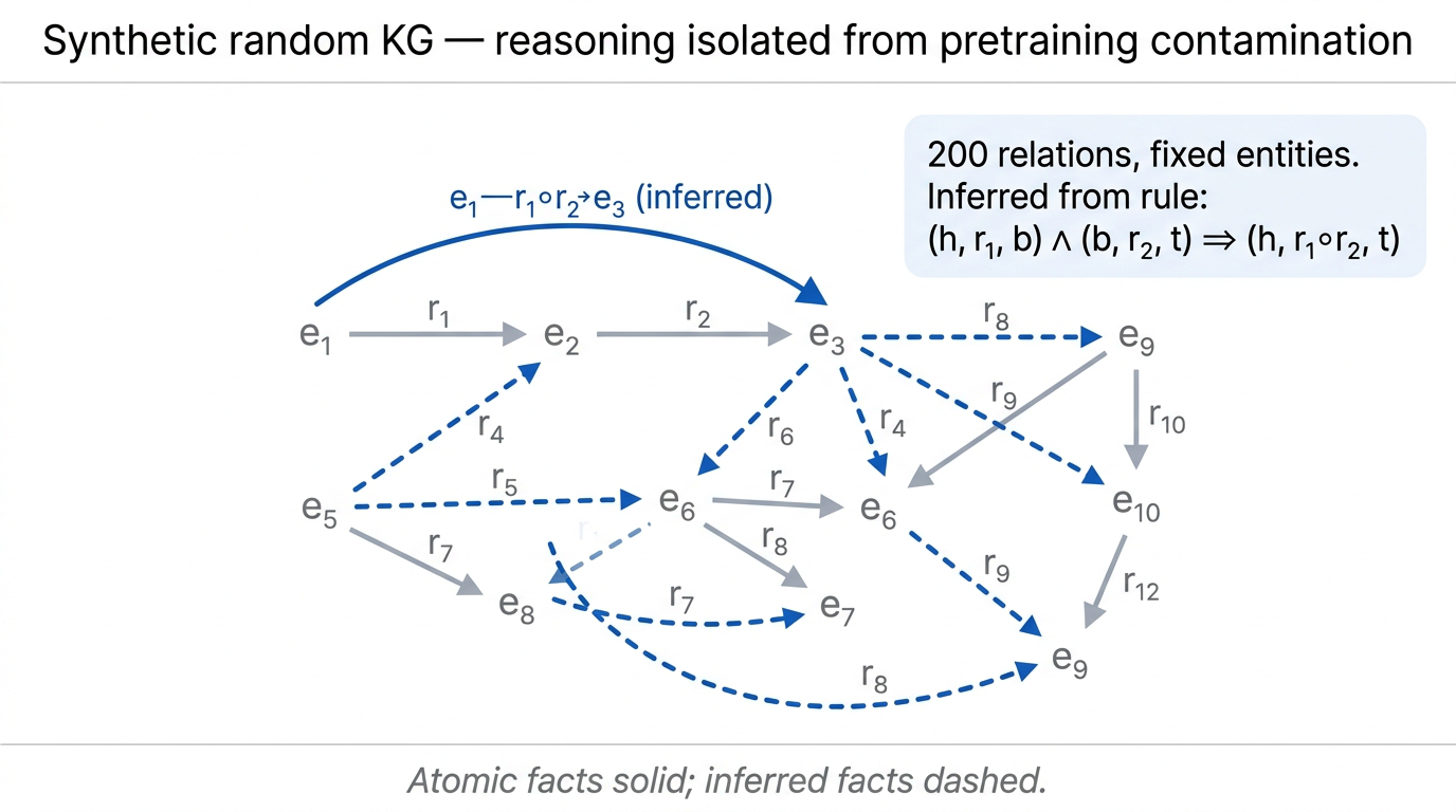
Fig 28. Random knowledge graph — atomic facts (single-hop) plus inferred facts generated via two-hop composition.

The data is random knowledge graphs with a fixed number of entities and 200 relations. Atomic facts are single-hop relations. Inferred facts come from a two-hop composition rule:

$$ (h, r_1, b) \wedge (b, r_2, t) \Rightarrow (h, r_1 \circ r_2, t) $$

Combining “Stevie Wonder is the singer of Superstition” with “Stevie Wonder’s place of birth is Michigan” yields the compositional fact connecting Superstition to Michigan via the composed relation “singer’s place of birth.”

The clever part is the data split. Atomic facts are divided into in-distribution (ID) and out-of-distribution (OOD) sets, each producing their own inferred facts.

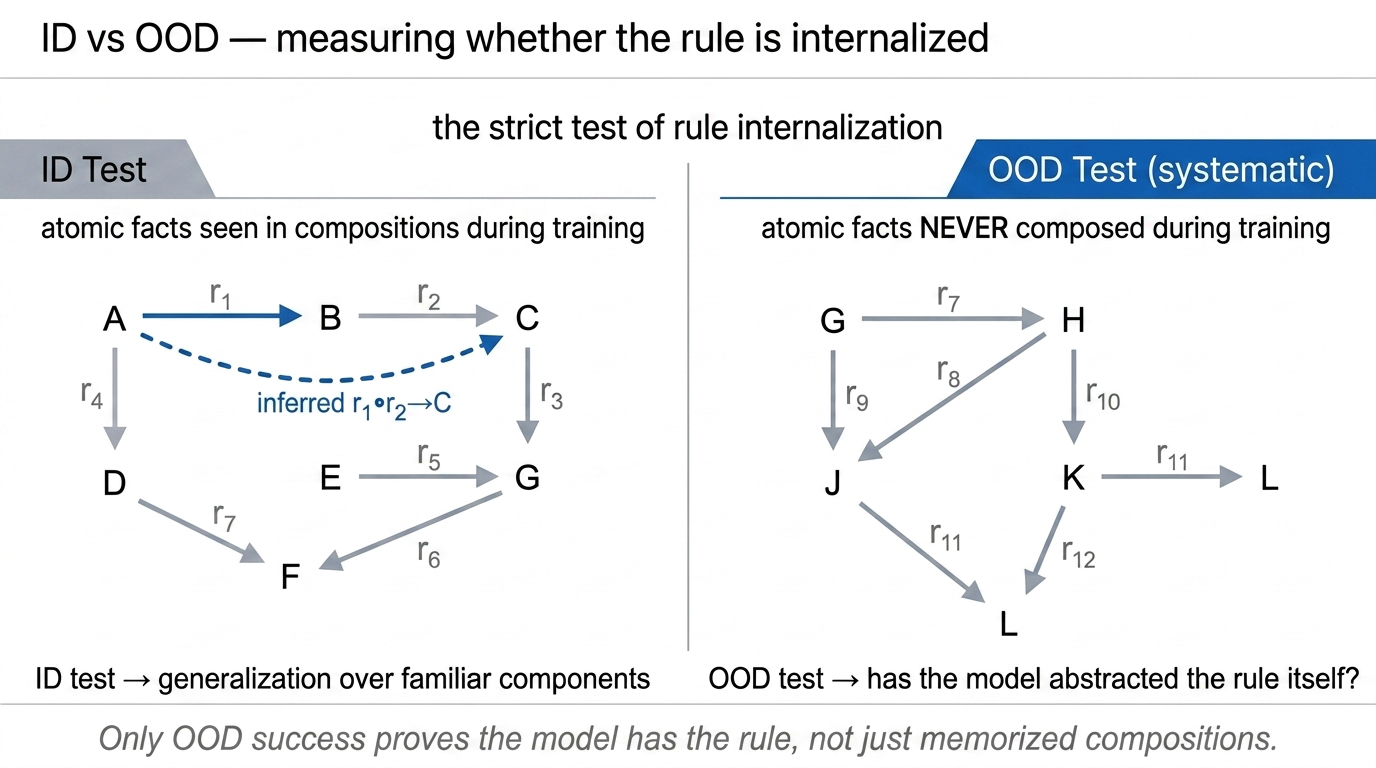
Fig 29. The inductive setup — ID test reuses atomic facts seen in compositions; OOD test uses atomic facts never composed during training.

Test type	What’s held out	What it measures
ID	Specific inferred fact combinations	Generalization over familiar components
OOD (systematic)	Atomic facts never composed in training	Whether the abstract rule is internalized

3.4 Three findings — grokking, systematicity, data distribution

Finding 1: Grokking is necessary for implicit reasoning. Transformers can learn to reason implicitly, but only through grokking — delayed generalization that happens long after the model has overfit the training data.

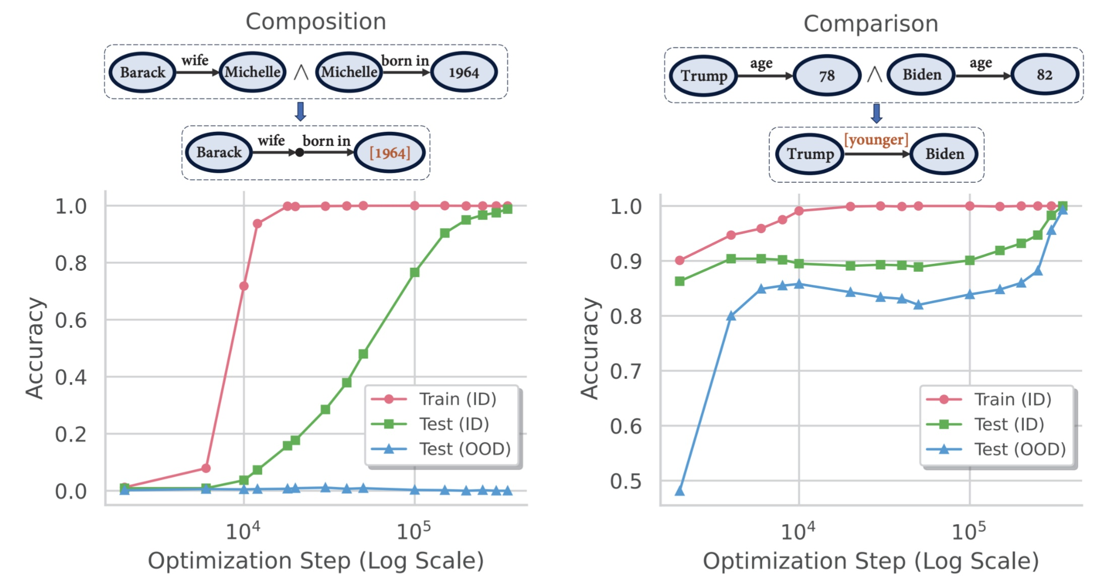
Fig 30. The grokking signature. Training accuracy hits 100% early, test accuracy lags badly, then suddenly jumps after roughly 20× more training.

For both composition and comparison tasks, training accuracy (red) hits 100% at around 10,000 optimization steps. Test accuracy (green) stays low. Only after roughly 20× more training does generalization suddenly emerge, with test accuracy jumping to near-perfect levels. The model memorizes first; if you keep training, it discovers the underlying reasoning pattern.

Finding 2: Systematicity depends on reasoning type. The degree of OOD generalization varies dramatically by what kind of reasoning is involved.

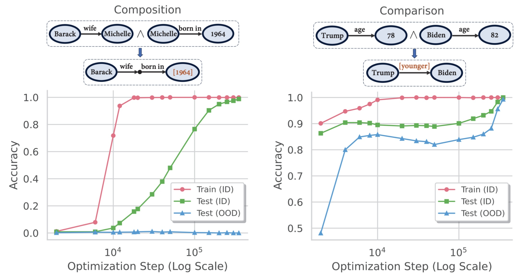
Fig 31. Same architecture, same training procedure, fundamentally different OOD behaviour. Composition fails OOD; comparison succeeds.

For compositional reasoning, OOD test accuracy never rises above near-zero, even after grokking on in-distribution data. For comparison reasoning, OOD generalization works — accuracy reaches 80–85%. Same architecture, same training procedure, completely different generalization behaviour.

Finding 3: Data distribution matters more than data size. The most counterintuitive result. The grokking literature often talks about a “critical dataset size” threshold beyond which grokking happens.

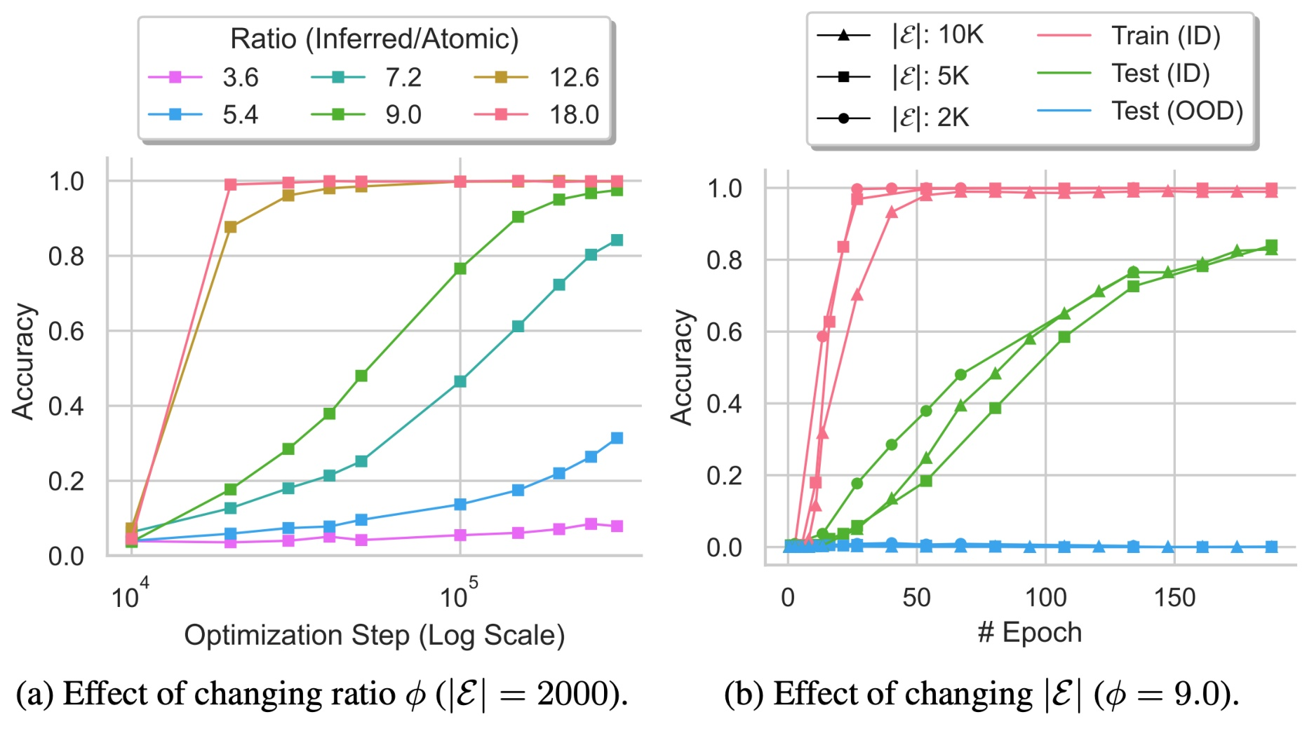
Fig 32. Panel (a) — increasing the inferred-to-atomic ratio \(\phi\) dramatically speeds up generalization. Panel (b) — increasing total data size with the ratio held fixed barely matters.

The experiments disentangle two variables: total data size (controlled by the number of entities \(|\mathcal{E}|\)) and data distribution (controlled by \(\phi\), the ratio of inferred facts to atomic facts). Increasing dataset size while holding the ratio fixed produces roughly the same generalization speed. Keep data size fixed but increase \(\phi\) from 3.6 to 18, and generalization speeds up dramatically.

Key idea: The composition of the training distribution, not its sheer volume, determines when implicit reasoning emerges. If you want a model to develop implicit reasoning, do not just add more data — change the mix. Tilt the distribution toward inferred facts that exercise the reasoning patterns you want.

3.5 Mechanistic analysis — circuit formation and the “aha moment”

Why does grokking happen? The team uses two interpretability tools. Logit lens projects internal states at any layer through the output embedding matrix, giving a peek at what the model “knows” at intermediate stages. Causal tracing quantifies how much each internal state actually influences the final prediction — a score closer to 1 means strong causal impact on the output.

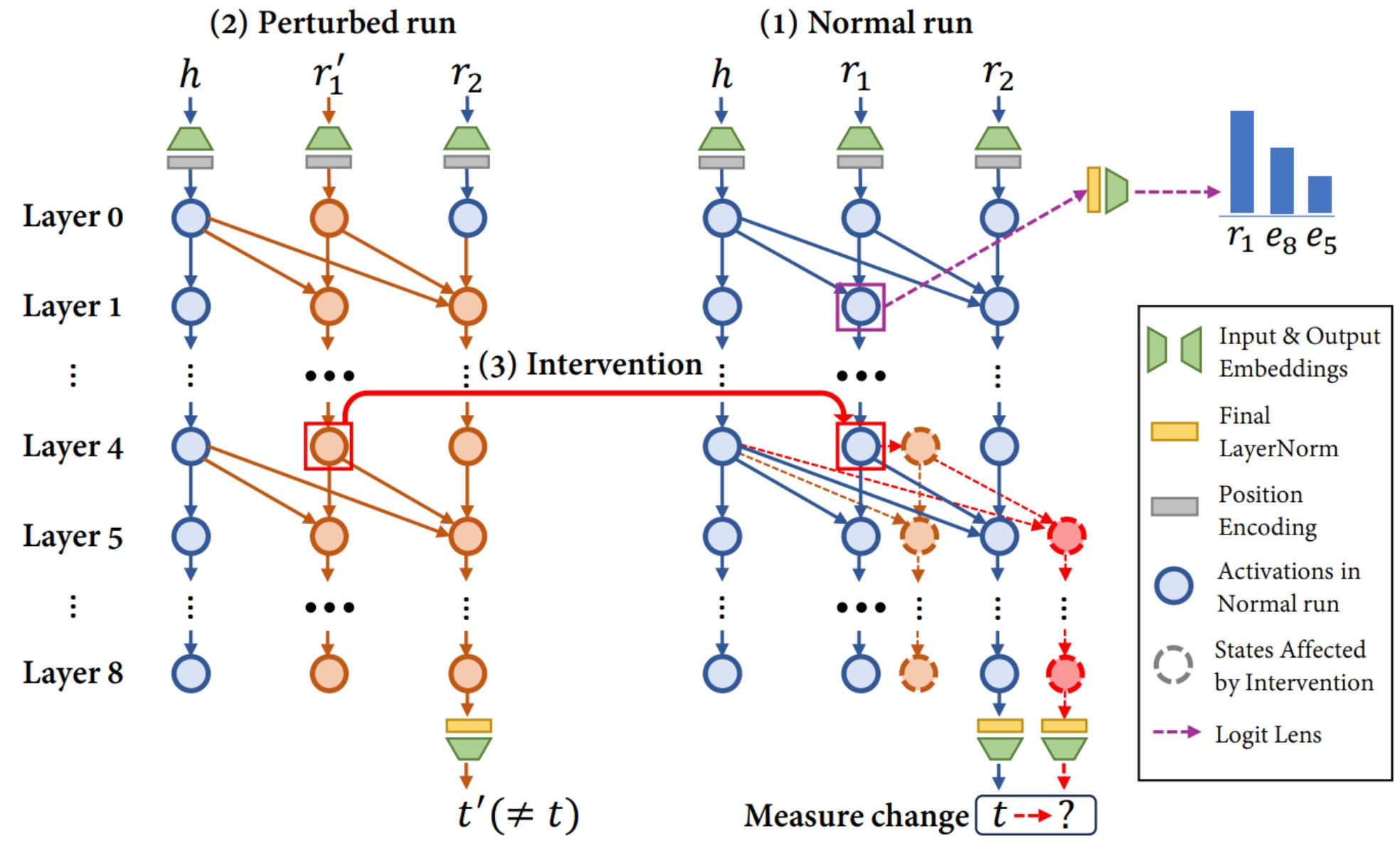
Fig 33. Causal tracing — compare a normal forward pass with a perturbed one to measure each intermediate state’s causal contribution.

Different reasoning types form distinctly different generalizing circuits after grokking — and the circuit configurations directly explain the difference in systematicity.

For composition reasoning, the model learns a staged circuit. The first few layers process the head entity and first relation to identify the bridge entity B. By layer 5, logit lens shows the model can reliably predict B. Crucially, the model also has to defer processing of the second relation \(r_2\), keeping it in reserve. Once B is identified, upper layers combine it with the delayed \(r_2\) to predict the tail entity T.

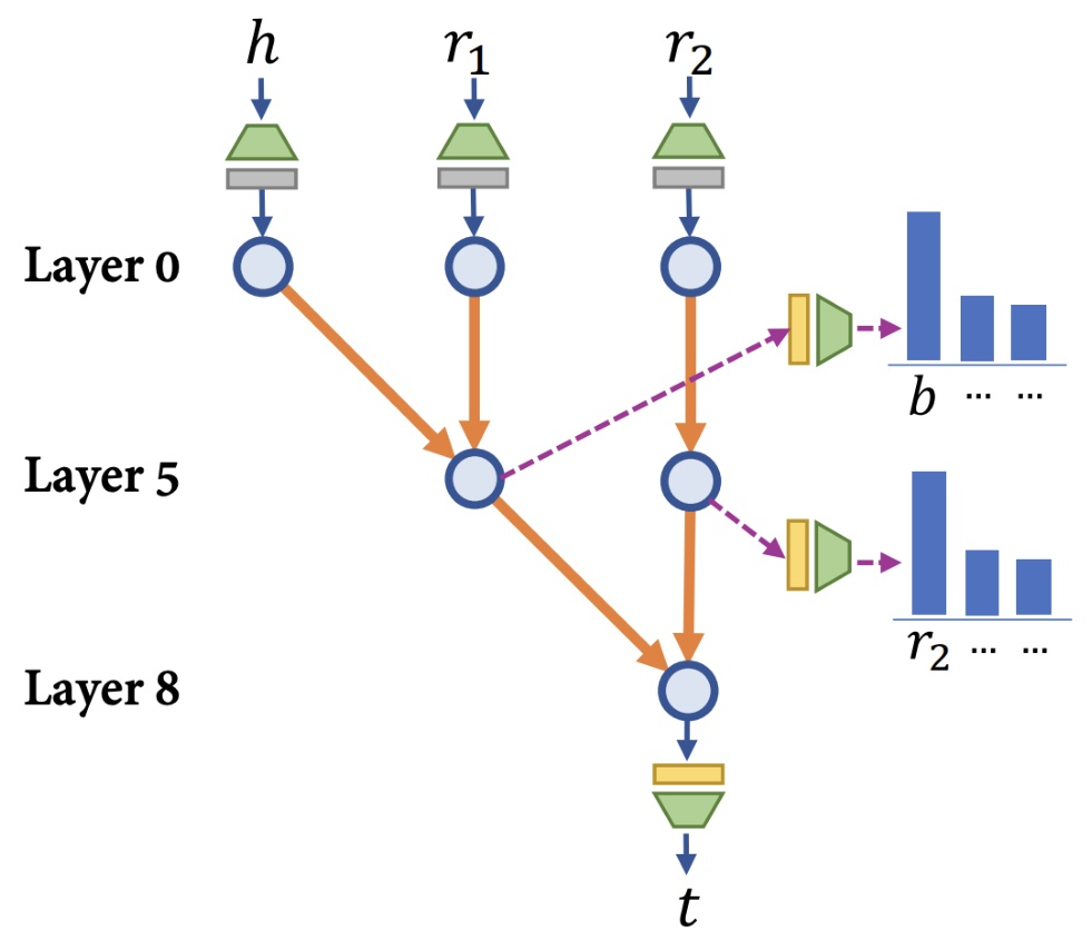
Fig 34. Staged composition circuit — bridge entity B identified in intermediate layers, then composed with the deferred second relation in upper layers.

Comparison reasoning, by contrast, forms a parallel circuit. The model retrieves both attribute values (e.g., the two release dates of GPT-4 and Claude 3) in parallel during the early layers, then upper layers perform the comparison op. No staging required.

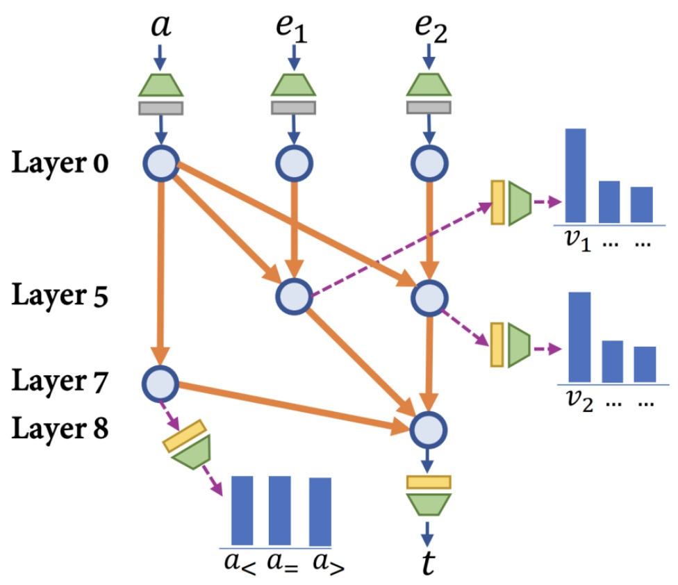
Fig 35. Parallel comparison circuit — attribute values retrieved in parallel, then compared.

Reasoning type	Circuit shape	OOD systematicity
Composition	Staged (sequential layers)	Fails (~0%)
Comparison	Parallel (concurrent retrieval)	Succeeds (~80–85%)

The staged circuit structure explains why composition fails OOD in the base setup. For OOD composition to work, the model needs to store atomic facts in both lower layers (for the first hop) and upper layers (for the delayed second hop). When atomic facts are never seen composed during training, there is no incentive to store them in the upper layers.

The clean intervention that validates this hypothesis: cross-layer parameter sharing. By tying the weights of lower and upper layers, atomic facts memorized in lower layers automatically appear in upper layers too. Result: OOD generalization for composition starts working.

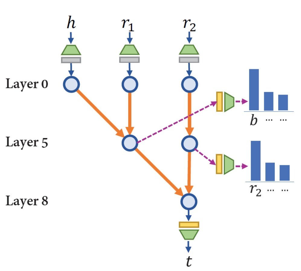
Fig 36. Cross-layer parameter sharing rescues OOD generalization for composition. Tying weights forces atomic facts to appear in both lower and upper layers.

The central insight: grokking is a phase transition from rote learning to generalization — the model’s “aha moment.” When grokking begins, the model has already overfit the training data. But it achieved that through pure memorization, not by forming the generalizing circuit.

Causal tracing reveals exactly what happens during the transition. At the start of grokking, the bridge entity B is already encoded at layer 5, position \(r_1\) — the mean reciprocal rank (MRR) is 1.0. But the MRR for \(r_2\) at the same position is near zero. The model has the bridge entity but is not using it — it is memorizing the mapping from \((h, r_1, r_2)\) to \(t\) directly.

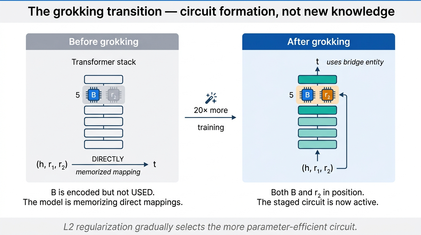
Fig 37. The grokking transition. Through training, the MRR for r₂ at the bridge position rises to 1.0, and causal tracing shows the model now routing through the bridge entity.

Through the grokking process, the MRR for \(r_2\) gradually increases until it hits 1.0. Now both B and \(r_2\) are properly positioned to execute the staged circuit. Causal tracing confirms it: the difference in causal strength before and after grokking is concentrated at the bridge entity position.

Key idea: Why does this transition happen? Circuit efficiency under L2 regularization. The generalizing circuit is far more parameter-efficient than rote memorization. Continuing to train past overfitting gradually favors the more efficient circuit. Training way beyond overfitting is not wasted — it is exactly when regularization sculpts the efficient generalizing circuit out of the memorized scaffolding.

---

4. Model-Based Planning — WebDreamer

4.1 Planning paradigms for language agents

Stripped-down definition: given a goal \(G\), planning decides on a sequence of actions \((a_0, a_1, \ldots, a_n)\) that will lead to a state passing the goal test \(g(\cdot)\).

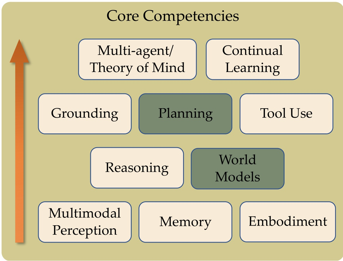
Fig 38. Where planning and world models sit in the language agent capability stack.

Compared to the classical planning settings studied for four decades, language agent planning shows three trends:

1. Goal specification is dramatically more expressive — natural language instead of formal languages with limited expressiveness.
2. Action space has expanded or become open-ended, well beyond constrained robotic primitives like “move forward” or “turn left.”
3. Automated goal testing has become hard or even infeasible in many scenarios.

Web agents make this concrete. A task like “Show me the reviews for the auto repair shop closest to ZIP 10002” uses plain natural language for the goal. The action space includes broad primitives — TYPE, CLICK, drag, hover — but the actual elements you interact with are dynamically populated on each webpage. Navigate to a different page and your action space changes entirely.

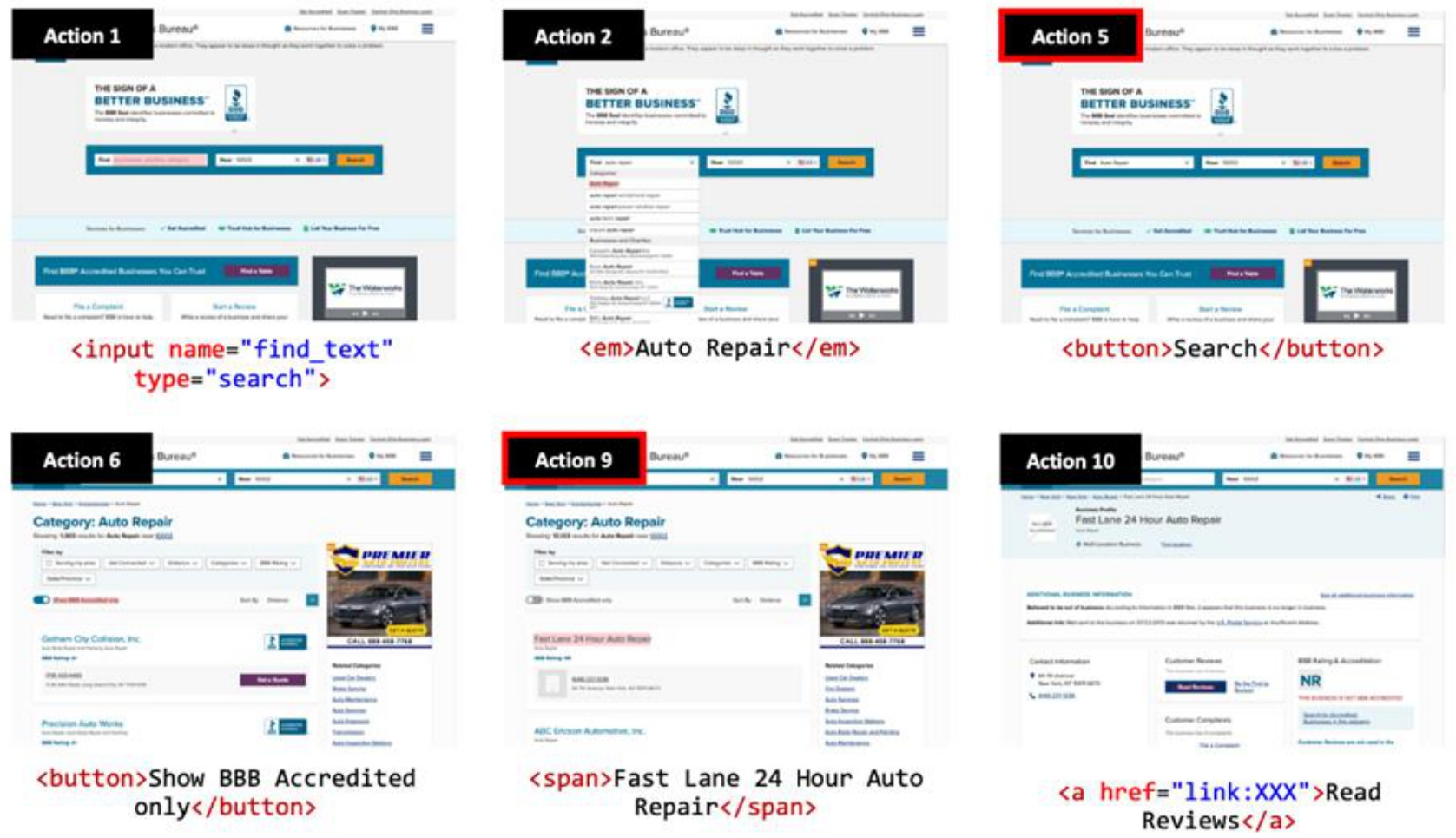
Fig 39. A web navigation sequence — each step’s action space comes from the current page’s DOM.

Travel planning has similar properties. A user specifies constraints — hard ones like budget and room type, plus commonsense ones like “reasonable route” or “diverse restaurants.” The agent has to orchestrate multiple tools (FlightSearch, AccommodationSearch, RestaurantSearch) and synthesize a multi-day itinerary. Writing an automated goal test ahead of time is essentially impossible.

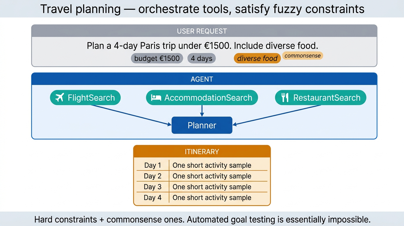
Fig 40. Travel planning architecture — constraint handling, tool orchestration, plan synthesis.

4.2 Reactive vs. tree search — the dilemma

The most common planning paradigm for language agents is reactive planning, also known as ReAct. At each state, the agent observes, reasons, picks an action, commits, transitions to the next state, repeats.

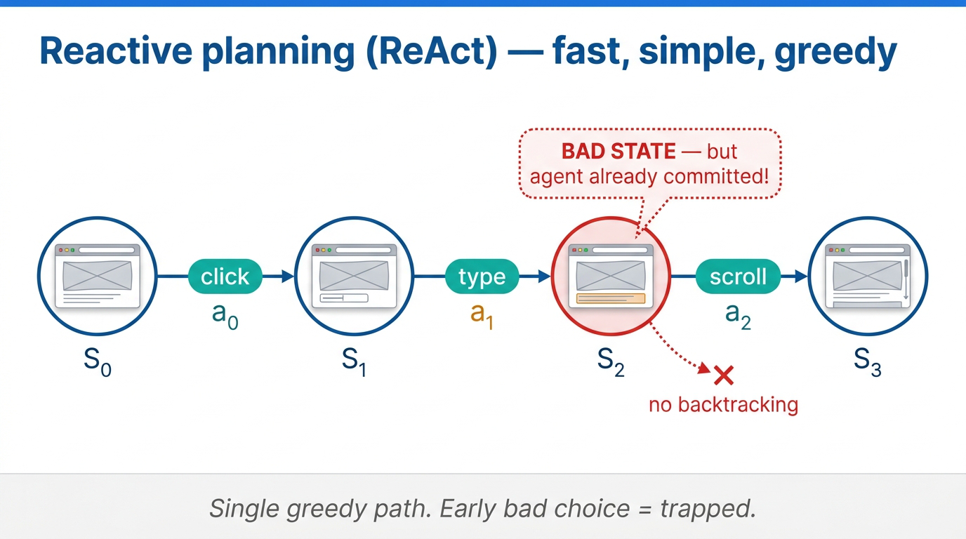
Fig 41. Reactive planning — a single greedy path through state space.

Reactive planning is fast and simple to implement, but it is fundamentally greedy and short-sighted. You can land in a bad state with no way out.

The natural alternative is tree search, which allows backtracking. Maintain values for states on the search frontier, expand promising branches, backtrack from unpromising ones.

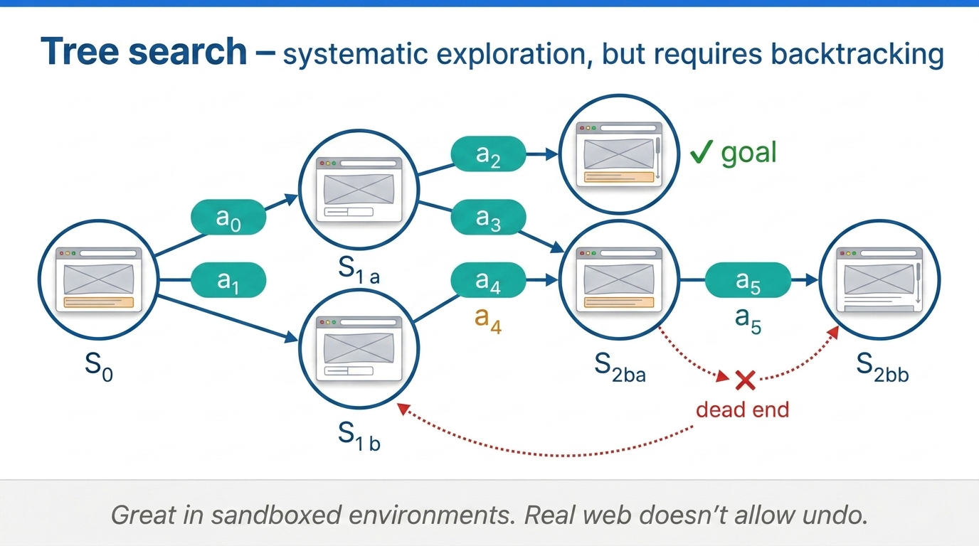
Fig 42. Tree search with real interactions — systematic exploration, but requires backtracking.

Systematic exploration sounds great in theory. In real-world environments like the internet, it runs into a serious problem: many actions are irreversible. You cannot just back out.

To get a sense of how pervasive state-changing actions are, consider Amazon alone. On a single website you can hit hundreds or thousands of irreversible actions: placing an order, making a return, creating an account (with legal implications), changing privacy settings.

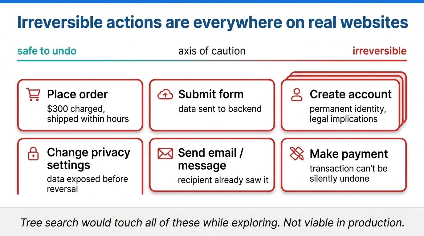
Fig 43. Real web workflows are full of state-changing, often irreversible actions.

Beyond technical impossibility, there are safety and cost issues. Exploring by actually executing actions can trigger unintended consequences, violate privacy, or incur real costs. Inference-time exploration becomes slow and expensive.

Approach	Speed	Quality	Safety	Real-world feasibility
Reactive (ReAct)	Fast	Greedy	OK	High
Tree search (real)	Slow	Systematic	Poor (irreversible actions)	Low
Model-based	Moderate	Systematic	Good (simulate first)	High

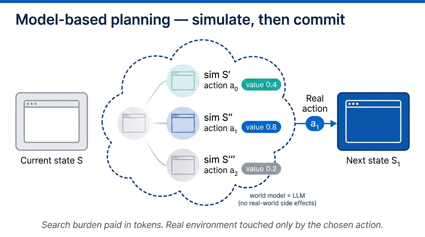
Fig 44. Model-based planning — simulate outcomes via a world model before committing to any real action.

The world model simulates the outcome of each candidate action. You can evaluate long-term value and safety before committing in the real environment. Find the most promising action through simulation, commit (assuming it is safe), reach a new state, repeat. Faster and safer than tree search with real interactions, while still enabling systematic exploration. The catch: you need that world model.

4.3 LLMs as world models of the internet

Building world models for language agents is harder than the classical RL setting. Atari games have simple, self-contained environments where you can run millions of trials. The internet does not.

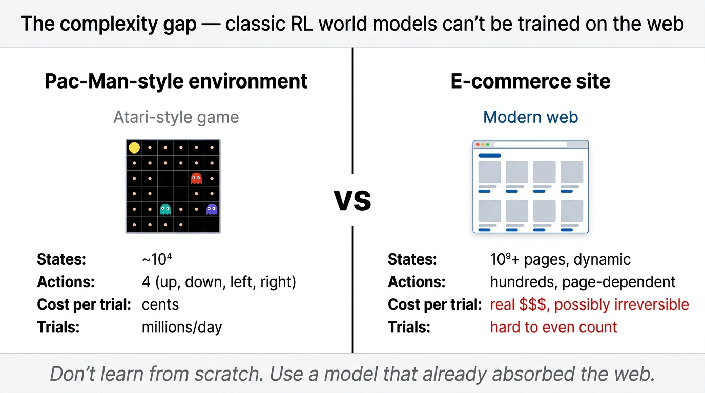
Fig 45. The complexity gap between classic RL environments and modern web interfaces.

A single website can have hundreds of pages, each with hundreds of possible actions. Pages constantly change as backend databases update. Multiply across billions of websites and the scale looks intractable.

The surprising insight: LLMs can already serve as approximate world models for the web. They have been trained on vast amounts of web data and have internalized common patterns about how websites behave. Show an LLM a product thumbnail on an e-commerce site and ask what happens when you click — the model predicts navigation to a product detail page with sizing options, customer reviews, and an “Add to Cart” button.

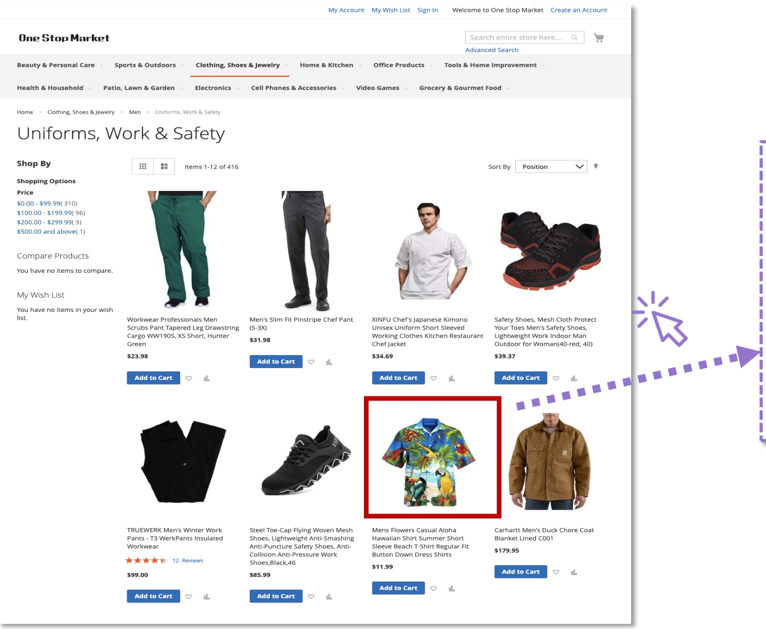
Fig 46. The LLM as a world model — predicting the next state from web conventions.

The model recognizes the shirt icon as a product element and uses its world knowledge to infer the likely next state. It understands e-commerce conventions — that product grids lead to detail pages, that clothing has size selectors. Not perfect prediction, but remarkably functional.

This transforms the planning problem. Instead of learning environment dynamics from scratch through trial and error, we use the LLM itself as a transition model:

$$ \hat{T} : S \times A \to S $$

The same model becomes both the policy (deciding what to do) and the world model (predicting what will happen).

4.4 WebDreamer — simulation-based planning in action

WebDreamer is a concrete instantiation of the LLM-as-world-model idea. It demonstrates this in practice. The world model is GPT-4o. When the agent is at a given state with several candidate actions, it uses the LLM to simulate the outcome of each action before committing. It can run multi-step simulations to look further ahead.

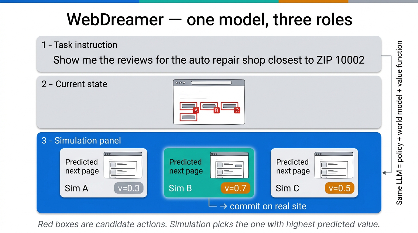
Fig 47. WebDreamer architecture — task instruction, current website state, and a simulation panel that predicts outcomes before any real action.

A value function — also implemented by the LLM — estimates how much progress each candidate action would make toward the goal. The agent picks the highest-valued action, transitions to the next state, repeats.

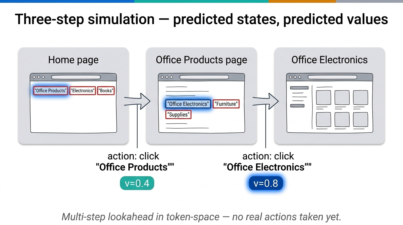
Fig 48. Three-step simulation — predicted webpage states and reward values at each decision point.

The process unfolds in two stages. Stage I — simulation: the agent predicts what will happen after each action. Clicking “Office Products” displays three sub-categories, then clicking “Office Electronics” shows products and a sub-menu. Each simulated step gets a value estimate (e.g., \(v = 0.4\), \(v = 0.8\)). Stage II — execution: the agent takes the highest-valued action on the real website and observes the actual outcome.

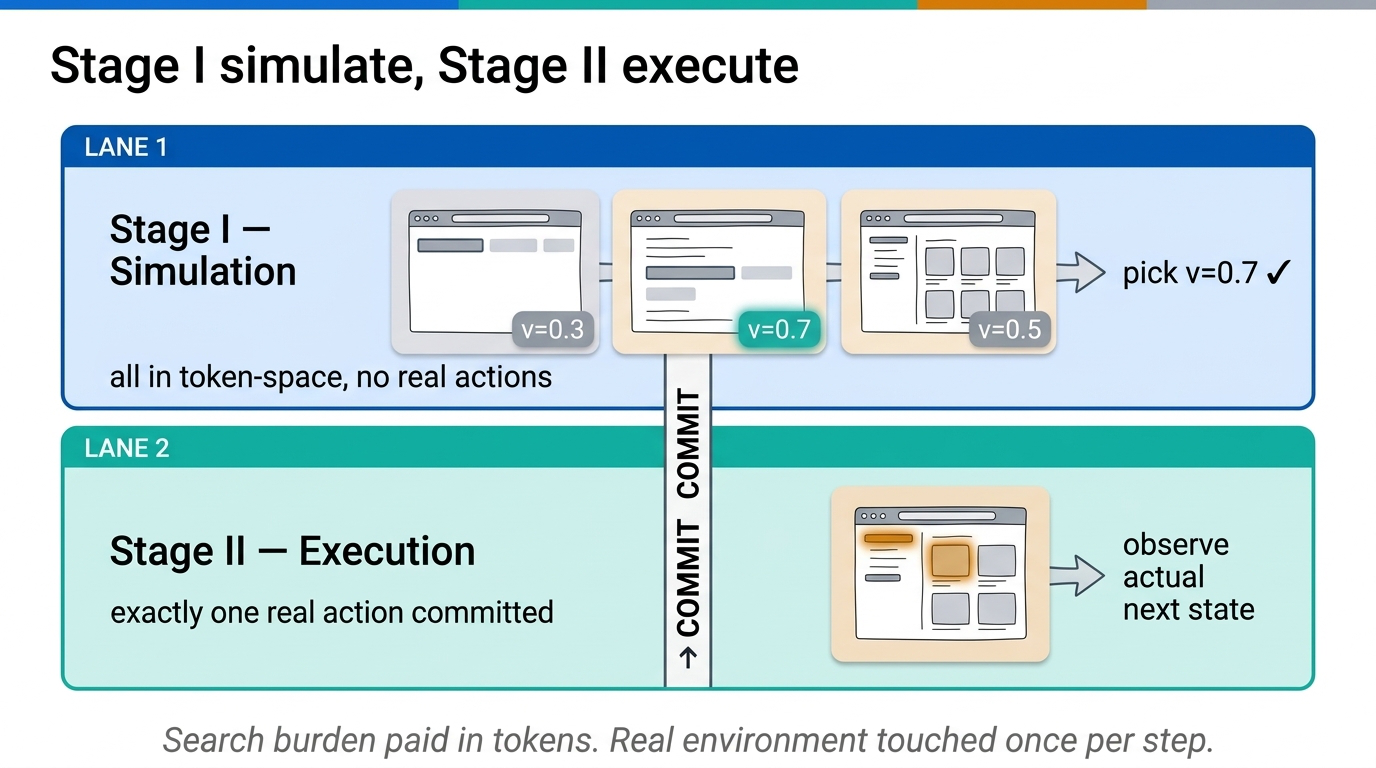
Fig 49. Stage I simulation with predicted outcomes and rewards; Stage II execution on the real site.

On VisualWebArena, model-based planning is more accurate than reactive planning and slightly trails tree search on success rate.

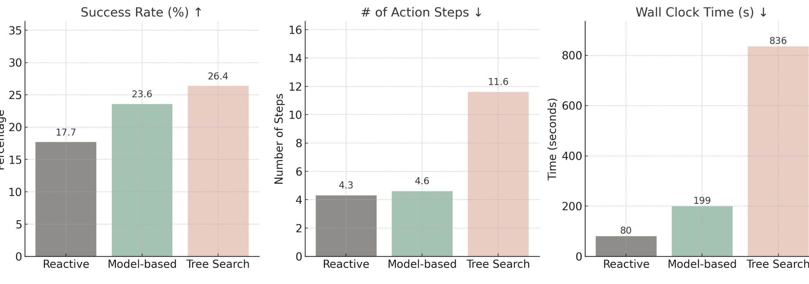
Fig 50. Model-based planning beats reactive planning on success rate (23.6% vs. 17.7%) and is far more efficient than tree search in steps and time — though it slightly trails tree search on raw success rate (26.4%).

The important caveat: tree search is only feasible in a sandbox environment like VisualWebArena. On real websites, backtracking is problematic — you cannot simply undo a purchase or form submission. Model-based planning is much cheaper and more practical for real-world deployment.

Key idea: The best planning strategy depends on the base LLM. Stronger models may need less scaffolding and can operate more reactively. How to improve planning in LLMs remains largely open. Many groups are exploring whether the recipe for o1/R1-style reasoning can be adapted for planning.

---

5. The Road Ahead and Open Challenges

Fig 51. Returning to the full capability stack — every box highlighted earlier is an open research problem worth deeper attention.

• Continual learning sits at the frontier. How does an agent continuously learn from its own use and exploration, building up personalized knowledge over time? Barely scratched.
• Reasoning — integrating o1/R1-style approaches into language agents. Core difficulty: agents operate in a fuzzy, real-world environment without the reliable reward signals that make RL work cleanly.
• Planning — better world models beyond simple LLM simulation, balancing reactive vs. model-based (you do not want to run expensive simulations at every step), sustaining long-horizon planning without losing focus.
• Safety — the most pressing concern. The attack surface of language agents is alarmingly broad. For web agents, it is essentially the entire internet.

Two general categories of safety risk:

Risk type	Origin	Example
Endogenous	Within the agent (incompetence)	Mistakenly takes irreversible harmful action
Exogenous	External environment	Adversarial attacks, prompt injection, manipulation

Despite the open problems, exciting applications are emerging. Agentic search / deep research has the clearest business case right now — Perplexity Pro, Google Deep Research. Workflow automation is another promising direction, as is agents for scientific discovery.

---

6. Appendix — Parametric vs. Non-Parametric Memory for Deep Reasoning

One last result worth surfacing, because it cuts against assumptions about RAG. The setup is a deliberately hard reasoning task — search space so large that even state-of-the-art LLMs with retrieval augmentation struggle.

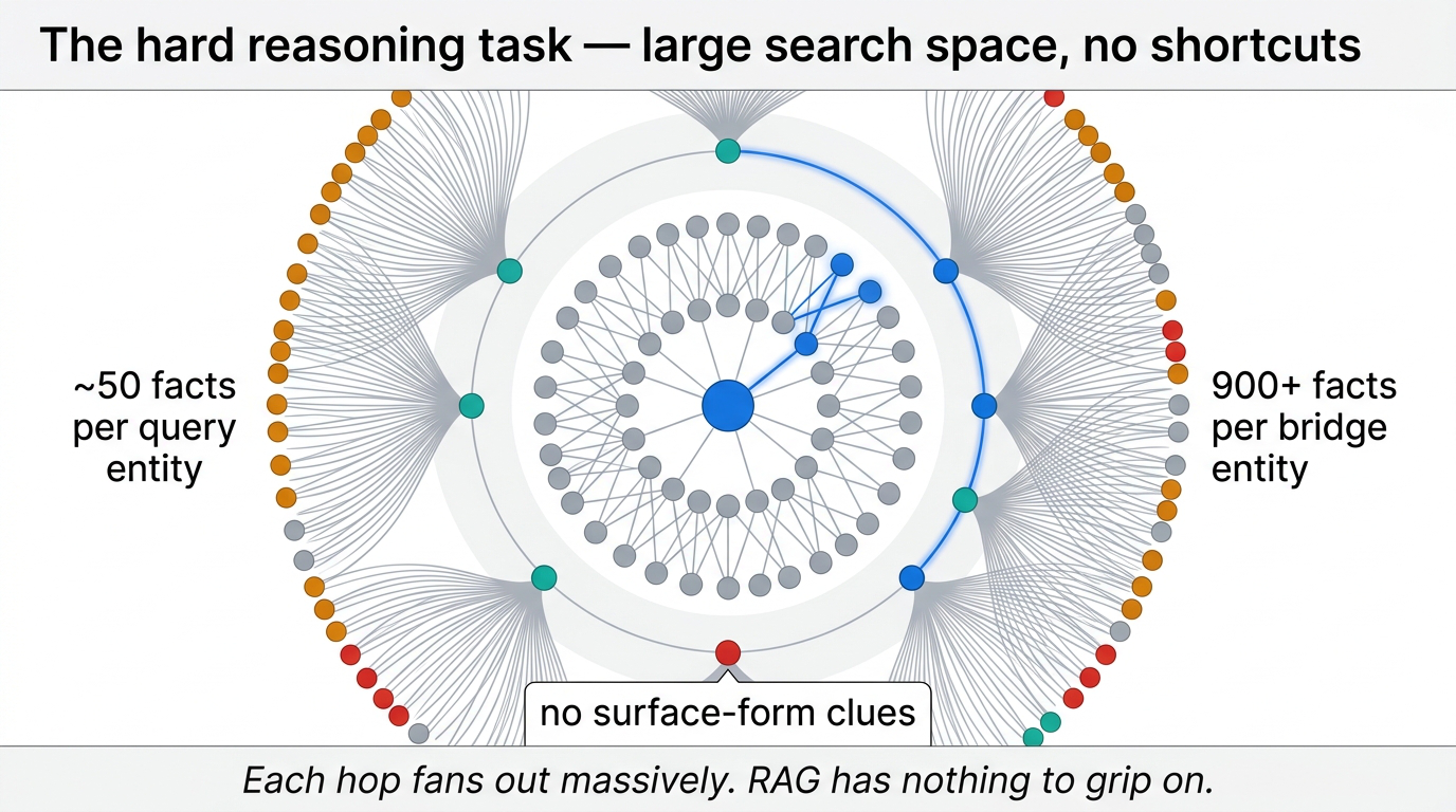
Fig 52. The hard setup — each query entity connects to ~50 facts, each bridge entity in the ground-truth proof connects to 900+, and there are no surface-form shortcuts.

Each query entity connects to roughly 50 facts. Each bridge entity in the ground-truth proof connects to over 900. Critically, there are no surface-form clues to exploit. This is unlike most QA benchmarks, where reasoning steps are relatively transparent.

When you test state-of-the-art LLMs with non-parametric memory (RAG) on this task, they fail badly. Even with chain-of-thought prompting and retrieval augmentation, GPT-4-Turbo and Gemini-Pro-1.5 only manage modest accuracy. There is also no major improvement from o1-preview or o3-mini (high).

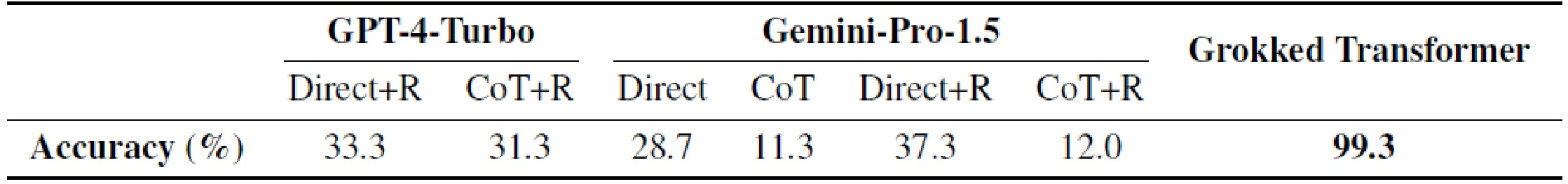
Fig 53. Accuracy on the deep-reasoning task — RAG-augmented frontier models struggle; a grokked transformer is near-perfect.

Model	Memory type	Accuracy
GPT-4-Turbo + CoT + RAG	Non-parametric	Modest
Gemini-Pro-1.5 + CoT + RAG	Non-parametric	Modest
o1-preview + RAG	Non-parametric	No major gain
o3-mini (high) + RAG	Non-parametric	No major gain
Grokked Transformer	Parametric	Near-perfect

The striking result: a grokked transformer that has fully internalized the facts into its parameters achieves near-perfect accuracy. Parametric memory, when knowledge is integrated and compressed deeply enough, navigates complex search spaces far more effectively than external retrieval.

Key idea: This is not an argument that parametric memory is always better. It is an argument that the choice between parametric and non-parametric memory depends on the structure of the reasoning the agent has to do. For complex multi-hop reasoning where the search space is vast and there are no easy heuristics, deeply encoded parametric knowledge appears to provide an advantage that current retrieval-augmented systems cannot match.

---

Source

Lecture: Reasoning, Memory & Planning of Language Agents by Yu Su (Ohio State University). Course: UC Berkeley CS294-280 Sp25 — Advanced Large Language Model Agents. Slides: PDF. Course page: rdi.berkeley.edu/adv-llm-agents/sp25.