#017 PyTorch – How to apply Batch Normalization in PyTorch

Highlights: Hello and welcome to our new post. Today, we’ll discuss another popular method used to improve the performance of your deep neural network called batch normalization. It is a technique for training deep neural networks that standardizes the inputs to a layer for each mini-batch. After finishing the theoretical part, we will explain how to implement batch normalization in Python using PyTorch. So, let’s begin with our lecture.
Tutorial Overview:
1. Data Normalization and standardization
How to normalize the data?
In order to understand batch normalization, first, we need to understand what data normalization is.
Data normalization is the process of rescaling the input values in the training dataset to the interval of 0 to 1. We need to normalize the data before we start training a neural network, during the pre-processing step, So, why do we need to transform our original data? Well, we need to do that because sometimes the data points may not be on the same scale. Therefore, we need to apply transformations in order to put all the data points on the same scale.
Now, let’s explore the normalization process in a little bit more detail.
For example, suppose we have a set of positive numbers from 0 to 100. To normalize this set of numbers we can just divide each number by the largest number in the set. In our case, it is the number 100. In that way, our data set has been rescaled to the interval from 0 to 1.

How to standardize the data?
Data standardization is a scaling technique used to establish the mean and the standard deviation of a normalized dataset. This method rescales data to have a mean of 0 and a standard deviation of 1 [1]. A typical standardization process consists of subtracting the mean of the dataset from each data point and then dividing the difference by the standard deviation of the dataset. Basically, we take every value \(x \) from the dataset and transform it to its corresponding \(z \) value using the following formula:
$$ z = x-mean/std $$
The mean of the data set is calculated using the following equation. It is a sum of all values divided by the number of values.
$$ \text { mean }=\frac{1}{N}\left(\sum_{i=1}^{N} x_{i}\right), $$
where \(N \) is the number of samples in the dataset.
To calculate the standard deviation the following equation is applied. We take the difference between each element and mean, square those differences, and then average the result. The standard deviation is just the square root of that result.
$$ std=\sqrt{\frac{1}{N}\left(\sum_{i=1}^{N}\left(x_{i}-mean\right)^{2}\right)}, $$
where \(N \) is the number of samples in the dataset.
After performing this computation on every \(x \) value in our dataset, we have a new standardized dataset of \(z \) values.
What is the goal of the normalization and standardization process?
In general, the purpose of both normalization and standardization is to put our data on the standardized scale. If we didn’t normalize our data, we may end up with some values in our data set that might be very high, and other values that might be very low.
This has the effect of stabilizing the learning process and dramatically reducing the number of training epochs required to train deep networks
For example, let’s say that we want to train our network to learn criteria according to which a certain company pays its employees. We have a data set which is a list of the company salaries from highest to lowest. Now imagine that in this dataset, we have someone with a salary of 1,000,000 dollars and someone else with a salary of only 1,000 dollars. This data has a relatively wide range and isn’t necessarily on the same scale. Additionally, each one of the features for our samples could vary widely as well. For example, we can have one feature, which corresponds to the age of the employee. In such a case we can also say that the salary and the age of the employee are not on the same scale.
This imbalance can cause instability in the neural network because features with larger values will have a bigger impact on the learning process compared with the features with smaller values. On the other hand, the normalized data will stabilize the learning process and can significantly decrease the number of epochs required to train deep neural networks.
So, now we learned how to normalize and standardize our data before we start training a neural network. However, there’s another problem that can arise even with normalized data. To solve this problem we need to apply batch normalization to individual layers within our network.
2. Batch normalization
When we normalize a dataset and start the training process, the weights in our model become updated over each epoch. So what will happen if, during training, one of the weights ends up becoming drastically larger than the other weight? This large weight can again cause the output from its corresponding neuron to be extremely large. Then, this imbalance will again continue to cascade through the neural network causing the problem where features with larger values will have a bigger impact on the learning process compared with the features with smaller values.

That is the reason why we need to normalize not just the input data, but also the data in the individual layers of the network. When applying batch norm to a layer we first normalize the output from the activation function. After normalizing the output from the activation function, batch normalization adds two parameters to each layer. The normalized output is multiplied by a “standard deviation” parameter \(\gamma \), and then a “mean” parameter \(\beta \) is added to the resulting product as you can see in the following equation.
$$ (z \cdot \gamma )+\beta $$
This calculation with the parameters \(\gamma \) and \(\beta \) sets a new standard deviation and mean for the data. These two parameters \(\gamma \) and \(\beta \) are also trainable, which means that they will also be optimized during the training process.
To sum up, when we apply standard normalization, the mean and standard deviation values are calculated with respect to the entire dataset. On the other hand, with batch normalization, the mean and standard deviation values are calculated with respect to the batch. This addition of batch normalization can significantly increase the speed and accuracy of our model.
Now, we learned the basic theory behind batch normalization. Let’s see how we can apply a batch norm in Python.
3. Batch normalization in PyTorch
In our experiment, we are going to build the LeNet-5 model. The main goal of LeNet-5 was to recognize handwritten digits. It was invented by Yann LeCun way back in 1998 and was the first Convolutional Neural Network.
This network takes a grayscale image as an input with dimensions of \(1\times32\times32 \) pixels. To train the model we are going to use the Fashion MNIST dataset which consists of 10 classes.
Then, we will create two networks. First, we are going to train the model without batch normalization. Then, we are going to create a second model, where the standard normalization and the batch normalization will be applied. Our goal is to train these two models and then compare their accuracy in order to see which one performed better. So, let’s begin with our experiment.
First, we need to import the necessary libraries. Then, We will define a variable called devices which will store CPU or GPU depending on what we are training on.
import matplotlib.pyplot as plt
import numpy as np
import datetime
import torch.optim.lr_scheduler as lr_scheduler

import torch
from torch import nn, optim
from torchvision import datasets, transforms
import torch.nn.functional as F
device = ("cuda" if torch.cuda.is_available() else "cpu") The next step is to download the Fashion MNIST for training and validation. We will use this data to train the first model where normalization and batch normalization will not be applied.
Here, we will use the function transforms.Compose() to apply several transformations. We are going to resize our images to the size of \(32\times32 \) pixels and then we are going to convert them into tensors using transforms.ToTensor() function.
transform1 = transforms.Compose([
          transforms.Resize((32, 32)),
          transforms.ToTensor()
          ])

train_set1 = datasets.FashionMNIST('DATA_MNIST/', download=True, train=True, transform=transform1)
trainloader1 = torch.utils.data.DataLoader(train_set1, batch_size=64, shuffle=True)

test_set1 = datasets.FashionMNIST('DATA_MNIST/', download=True, train=False, transform=transform1)
testloader1 = torch.utils.data.DataLoader(test_set1, batch_size=64, shuffle=True)

train_data_size = len(train_set1)
test_data_size = len(test_set1)
With the following code, we can extract and display one image from our dataset. Note that you need to reshape the tensor image of the shape \(64\times1\times32\times 32 \) to the shape of \(32\times32 \).
tensor_image1, index_label = test_set1[50]
new_img1 = np.transpose(tensor_image1, (1,2,0)).reshape((32,32))
plt.imshow(new_img1)

Also, let’s visualize the distribution of the pixels values in this non-normalized image.
# convert image to numpy array
img_np1 = np.array(new_img1)

# plot the pixel values
plt.hist(img_np1.ravel(), bins=50, density=True)
plt.xlabel("pixel values")
plt.ylabel("relative frequency")
plt.title("distribution of pixels")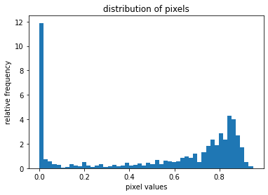
As you can see, the pixel values from the non-normalized image are distributed in a range from 0 to 1. Now, let’s create data for our second model. Everything will remain the same only this time we will normalize the data.
For our second model, we are going to apply one additional function transforms.Normalize(). The parameters for this function are mean and std. So, before we apply this function, we need to calculate mean and std for our dataset.
To calculate mean and std we are going to create the function mean_std(). We will iterate through images in trainloader and create variables sum, squared_sum and num_batches. In the variable sum we will store the sum of all mean values of the data, and in the variable squared_sum we will store all squared mean values. Then we will simply calculate mean and std for the Fashion MNIST dataset using the following equations:
$$ \text { mean }=\frac{1}{N}\left(\sum_{i=1}^{N} x_{i}\right) $$
$$ std=\sqrt{\frac{1}{N}\left(\sum_{i=1}^{N}\left(x_{i}-mean\right)^{2}\right)} $$
def mean_std(loader):
  sum, squared_sum, num_batches = 0,0,0
  for data,_ in loader:
    sum += torch.mean(data,dim=[0,2,3])
    squared_sum += torch.mean(data**2,dim=[0,2,3])
    num_batches += 1
  mean = sum/num_batches
  std = (squared_sum/num_batches - mean**2)**0.5
  return mean, std
Now, we will call our function and print the results.
mean,std = mean_std(trainloader)
print(mean)
print(std)
Output:
tensor([0.2856])
tensor([0.3385])
As you can see, the mean is equal to 0.2856, and the standard deviation is equal to 0.3385. When we add these values to the function transforms.Normalize(), we will normalize every pixel in our data set.
The next step is to download our dataset and create trainloader and testloader objects using the function torch.utils.data.DataLoader(). As parameters we will pass our dataset, we will set the batch size to 64 and finally, we will shuffle the data.
transform2 = transforms.Compose([
          transforms.Resize((32, 32)),
          transforms.ToTensor(),
          transforms.Normalize((mean),(std))
          ])

train_set2 = datasets.FashionMNIST('DATA_MNIST/', download=True, train=True, transform=transform2)
trainloader2 = torch.utils.data.DataLoader(train_set, batch_size=64, shuffle=True)

test_set2 = datasets.FashionMNIST('DATA_MNIST/', download=True, train=False, transform=transform2)
testloader2 = torch.utils.data.DataLoader(test_set, batch_size=64, shuffle=True)

train_data_size = len(train_set2)
test_data_size = len(test_set2)
Now, let’s extract and display the same image from the normalized dataset, and plot the pixel values distribution.
tensor_image2, index_label = test_set2[50]
new_img2 = np.transpose(tensor_image2, (1,2,0)).reshape((32,32))
plt.imshow(new_img2)
# convert image to numpy array
img_np2 = np.array(new_img2)

# plot the pixel values
plt.hist(img_np2.ravel(), bins=50, density=True)
plt.xlabel("pixel values")
plt.ylabel("relative frequency")
plt.title("distribution of pixels")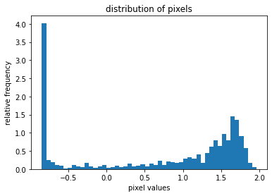
As you can see, the normalized pixel values in the image are now in the range between -1 and 2.
Next, we will extract one batch from the training set, to check the shape of our images, We can see that we have 64 images of the shape 1x32x32 pixels, and also we have 64 labels.
training_data = enumerate(trainloader)
batch_idx, (images, labels) = next(training_data)
print(images.shape) # Size of the image
print(labels.shape) # Size of the labels
Output:
torch.Size([64, 1, 32, 32])
torch.Size([64])
Now let’s take a look at the architecture of our two neural networks.
The first model is called LeNet5 and it is a standard model without batch normalization. It consists of the following layers.
Layer 1 (C1): First convolutional layer with 6 kernels of size \(5 \times 5 \) and stride of 1. The input size to this layer is \(32\times32 \times1 \) and the output is of size \(28\times28\times1 \) .
Layer 2 (S2): MaxPooling layer with 6 kernels of size \(2\times2 \) and stride of 2. The output of this layer is of size \(14\times14 \times 6 \)
Layer 3 (C3): Another convolutional layer, same configurations, just with 16 filters. Output is of size \(10\times10 \times 16 \)
Layer 4 (S4): MaxPooling layer, again with the same configurations as the previous, just with 16 filters. Output is \(5\times5 \times 16 \)
Layer 5 (F5): First fully-connected layer. It returns 120 units, and the ReLU activation function.
Layer 6 (F6): Second fully-connected layer. It takes 120 units and returns 84, and for the activation function, we will use the softmax function.
class LeNet5(nn.Module):

    def __init__(self):
        super(LeNet5, self).__init__()

        self.convolutional_layer = nn.Sequential(
            nn.Conv2d(in_channels=1, out_channels=6, kernel_size=5, stride=1),
            nn.ReLU(),
            nn.MaxPool2d(kernel_size=2, stride=2, padding=0),
            nn.Conv2d(in_channels=6, out_channels=16, kernel_size=5, stride=1),
            nn.ReLU(),
            nn.MaxPool2d(kernel_size=2, stride=2, padding=0),
            nn.Conv2d(in_channels=16, out_channels=120, kernel_size=5, stride=1),
            nn.ReLU()
        )

        self.linear_layer = nn.Sequential(
            nn.Linear(in_features=120, out_features=84),
            nn.ReLU(),
            nn.Linear(in_features=84, out_features=10),
        )


    def forward(self, x):
        x = self.convolutional_layer(x)
        x = torch.flatten(x, 1)
        x = self.linear_layer(x)
        x = F.softmax(x, dim=1)
        return x
Now, the second model is called LeNet5_norm, and it’s very similar to the first one. The only difference is that now we are going to apply batch normalization. To do this we will use the function BatchNorm2D(). The first batch norm will be applied after the first MaxPooling layer. Note, that we are using 2D because here we are dealing with two-dimensional images.
Next, we need to specify the number of the input channels to the batch norm layer. This number will be equal to the number of output channels in the convolutional layer.
After that, we will apply another batch norm to the linear layer. Here, we will use the BatchNorm1D() function because our data is already been flattened. Again, the number of the input channels will be the same as the number of output channels in the linear layer which, in this case, is equal to 84.
class LeNet5_norm(nn.Module):

    def __init__(self):
        super(LeNet5_norm, self).__init__()

        self.convolutional_layer = nn.Sequential(
            nn.Conv2d(in_channels=1, out_channels=6, kernel_size=5, stride=1),
            nn.ReLU(),

            nn.MaxPool2d(kernel_size=2, stride=2, padding=0),
            nn.BatchNorm2d(6),

            nn.Conv2d(in_channels=6, out_channels=16, kernel_size=5, stride=1),
            nn.ReLU(),
            nn.MaxPool2d(kernel_size=2, stride=2, padding=0),
            nn.Conv2d(in_channels=16, out_channels=120, kernel_size=5, stride=1),
            nn.ReLU()
        )

        self.linear_layer = nn.Sequential(
            nn.Linear(in_features=120, out_features=84),
            nn.ReLU(),
            nn.BatchNorm1d(84),
            nn.Linear(in_features=84, out_features=10),
        )


    def forward(self, x):
        x = self.convolutional_layer(x)
        x = torch.flatten(x, 1)
        x = self.linear_layer(x)
        x = F.softmax(x, dim=1)
        return x
After building the network we will just call the model and set it to work on the device we defined in the beginning.
model1 = LeNet5().to(device)
model2 = LeNet5_norm().to(device)
The next step is to optimize the weights and biases. Therefore we need to define the optimizer and criterion. To calculate the gradients, we will use the optim.Adam() function. As parameters to this function, we will pass the model.parameters(), and we will set the learning rate to be equal to 0.001. Then, we will calculate the loss by using the nn.CrossEntropyLoss() function.
Another important thing that we need to specify is the learning rate scheduler. The reason for that is that we don’t want that our learning rate stays constant. What we want is that the learning rate to decrease. To achieve our goal we will apply the method called stepLR. This method decays the learning rate by the value of gamma every step_size epochs. In our example, step_size is set to 5. That means that the initial learning rate will drop every 5 epochs by the value of gamma. To find out more about the learning rate schedule, click on this link.
optimizer = optim.Adam(model.parameters(), lr=0.001)
scheduler = torch.optim.lr_scheduler.StepLR(optimizer, step_size= 5, gamma=0.1)
criterion = nn.CrossEntropyLoss()
Now let’s train our two models and see whether the results differ.
epochs = 30
train_loss = []
val_loss = []
t_accuracy_gain = []
accuracy_gain = []

for epoch in range(epochs):

    total_train_loss = 0
    total_val_loss = 0

    model.train()
    total_t = 0
    # training our model
    for idx, (image, label) in enumerate(trainloader):

        image, label = image.to(device), label.to(device)
        optimizer.zero_grad()
        pred_t = model(image)

        loss = criterion(pred_t, label)
        total_train_loss += loss.item()

        loss.backward()
        optimizer.step()

        pred_t = torch.nn.functional.softmax(pred_t, dim=1)
        for i, p in enumerate(pred_t):
            if label[i] == torch.max(p.data, 0)[1]:
                total_t = total_t + 1

    accuracy_t = total_t / train_data_size
    t_accuracy_gain.append(accuracy_t)


    total_train_loss = total_train_loss / (idx + 1)
    train_loss.append(total_train_loss)

    # validating our model
    model.eval()
    total = 0
    for idx, (image, label) in enumerate(testloader):
        image, label = image.to(device), label.to(device)
        pred = model(image)
        loss = criterion(pred, label)
        total_val_loss += loss.item()

        pred = torch.nn.functional.softmax(pred, dim=1)
        for i, p in enumerate(pred):
            if label[i] == torch.max(p.data, 0)[1]:
                total = total + 1

    accuracy = total / test_data_size
    accuracy_gain.append(accuracy)

    total_val_loss = total_val_loss / (idx + 1)
    val_loss.append(total_val_loss)

    #if epoch % 5 == 0:
    print('\nEpoch: {}/{}, Train Loss: {:.4f}, Val Loss: {:.4f}, Val Acc: {:.4f}'.format(epoch, epochs, total_train_loss, total_val_loss, accuracy))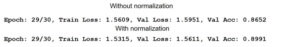
As you can see, we achieved the validation accuracy of almost 86.5% with the model where batch normalization was not applied. This is a pretty good result especially because training accuracy tends to increase if we continue training for more epochs.
However, the model where batch normalization was applied achieved a validation accuracy of almost 90%. This is a 3 % improvement compared with a model without batch norm.
Also, if we take a look at the following image, we can see that the batch norm model has much faster convergence. This means that it reaches a minimum much faster than the model without batch norm.


Furthermore, we can see that at the 10th epoch the model without batch norm achieved 85% accuracy while the batch norm model at the same epoch achieved an accuracy of 89%.
So, we can conclude that applying a normalization and batch normalization can be very useful and can help you to improve the performance of your model.
Summary
So, that is all for this lecture. In this post, we talked about methods called normalization, standardization, and batch normalization. We learned when we need to use these methods, and why applying them can help our network to preformed better and faster.