#016 PyTorch – Three hacks for improving the performance of Deep Neural Networks: Transfer Learning, Data Augmentation, and Scheduling the Learning rate in PyTorch

Highlights: Hi and welcome to our new post. In this post, we are going to talk about very popular deep learning techniques that we can apply to speed up training and improve the performance of our deep learning model. You will learn how you can use transfer learning and some other popular methods like data augmentation and scheduling the learning rate. So, let’s begin.
Tutorial Overview:
1. What is transfer learning?
Transfer learning is an incredibly powerful technique where pre-trained models are used as the starting point on computer vision and natural language processing tasks. So in other words, a network trained for one task is adapted to another task.
With transfer learning, you’re likely to spend much less time in training. For example, let’ say that you have a small training dataset with just a few hundred images. In such a case, you can apply transfer learning and you will be able to improve the performance of your deep learning model.
When building a computer vision application, rather than training a neural network from scratch, we often make much faster progress if we download the network’s weights. In other words, someone else has already trained the network architecture and we can use that for a new task that we are solving.
So, let’s say that we are developing a neural network for the pre-trained smile detector. Here, we have a classification problem with only 2 classes: smile and nonsmile. Now let’s say that our training set is quite small and we didn’t achieve great accuracy. So, what can we do in that case? Well, the computer vision research community has posted lots of datasets on the internet like Imagenet or NS Coco, or Pascal datasets. So, we can use transfer learning to transfer knowledge from some of these very large public datasets to our own problem.
Now, let’s take the Imagenet dataset as an example. It has 1000 different classes. The network might have a softmax unit that outputs one of a thousand possible classes. What we can do is get rid of the softmax layer and create a softmax unit that suits our own purpose with only 2 classes.
To better understand this let’s take a look at the following image.
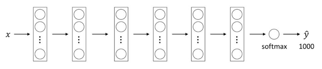
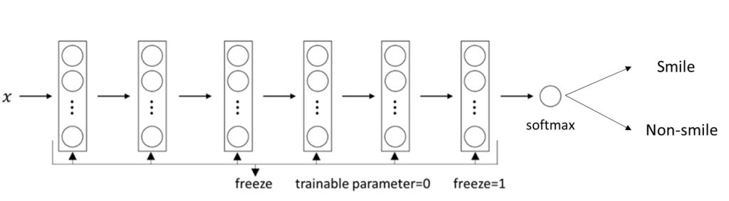
As you can see in the illustration above, we have used the model that has already been trained. Then, after we have modified only the last layer, we can use a new model to classify whatever we want. This is very useful because training a completely new model can be extremely time-consuming.
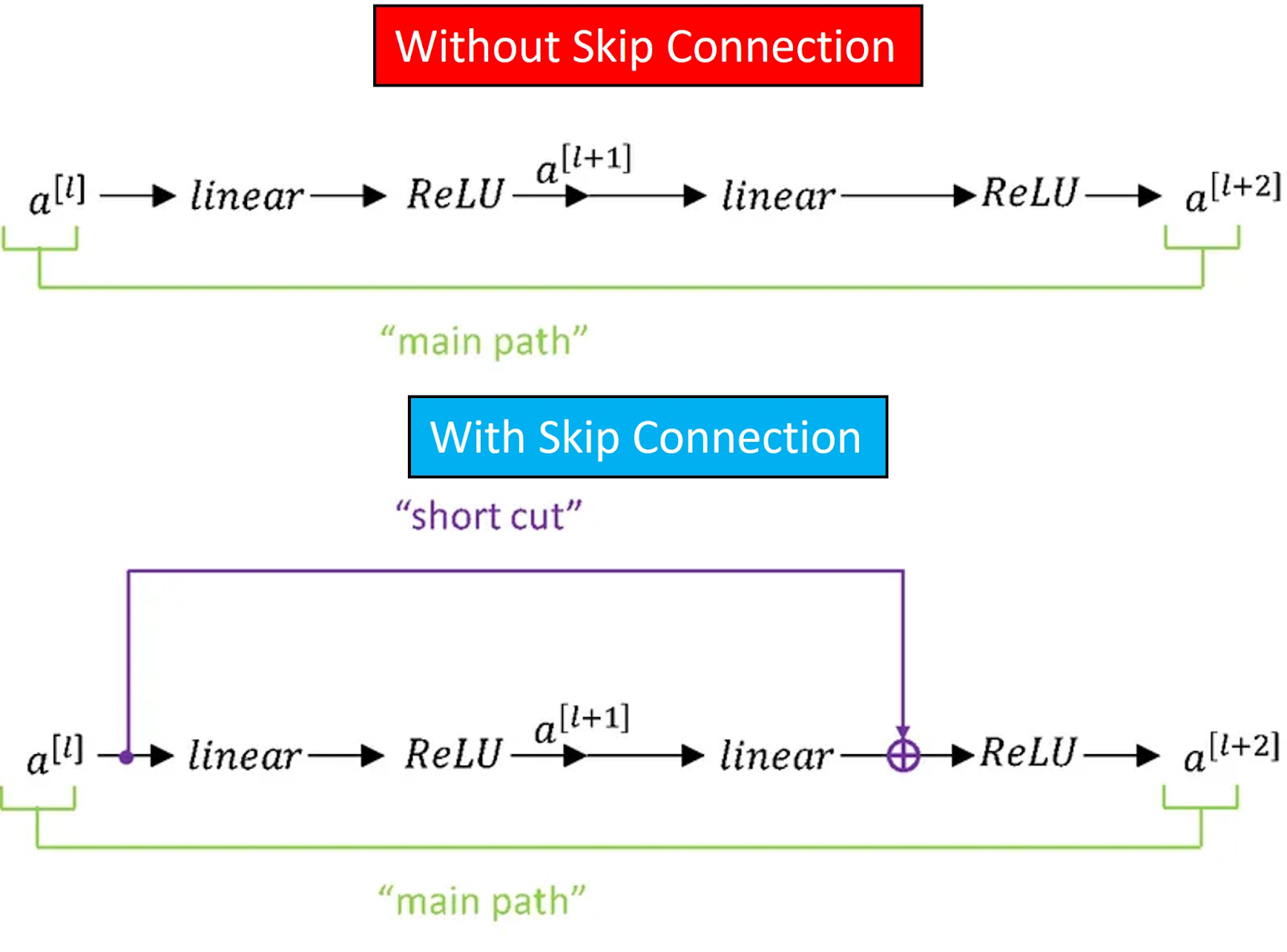
Multi-layer deep neural networks are difficult to train and can often produce other unexpected results. For example, the training accuracy drops as the number of layers increase. This problem is known as vanishing gradients. To solve this problem we can use Residual networks that will help us to skip connections. In other words, we can use shortcuts and take the activation from one layer and feed it to another layer much deeper in the neural network as we can see in the following examples. To learn about Residual networks in more detail check out our post Residual nets.
There are different versions of ResNet, including ResNet-18, ResNet-34, ResNet-50, and so on. The numbers denote layers, although the architecture is the same.
Now let’s take a look at an example in PyTorch.
Transfer learning in PyTorch
We are going to use a pre-trained ResNet18 network. This network is trained on millions of images of the Imagenet database. It is 18 layers deep and can classify images into 1000 categories.
In our example, we are going to use a trained LeNet5 model for a smile detector. So let’s begin with our code and use transfer learning to improve the accuracy of our model.
The first step is to import the ResNet model. Next, we load the resnet18 model and specify the parameter pretrained to True.
from torchvision import models
model = models.resnet18(pretrained=True)
Now, when we have downloaded our ResNet model we need to replace the fully connected layer with 1000 classes with a new layer with only 2 classes. First, we will specify the number of input features from the last layer. The next step is to create a new layer and assign it to the last layer in our model. Finally, we are going to send our model to the device.
n_f = model.fc.in_features
model.fc = nn.Linear(n_f, 2)
model.to(device)
The fully connected layer is now successfully replaced and we are ready to train our model. The next step is to optimize the weights and biases. Therefore we need to define the optimizer and criterion. For an optimizer, we will use the optim.Adam() function which will calculate gradients. As parameters to this function, we will pass the model.parameters(), and we will set the learning rate to be equal to 0.001. Then, we will calculate the loss by using nn.CrossEntropyLoss() function.
optimizer = optim.Adam(model.parameters(), lr=0.001)
criterion = nn.CrossEntropyLoss()
In this way, we have created a structure that does not require training of all layers but only the last layer. We created the model Now, we are ready to train the model. But before we begin with training let’s explore some other techniques that will help us to improve the performance of our classifier.
2. Scheduling the Learning rate
One of the most important hyperparameters that we need to set when training a neural network is the learning rate for the optimization algorithm. This parameter is a very small number usually ranging between 0,1 and 0,0001 and it scales the magnitude of our weight updates in order to minimize the network’s loss function. Often during the training process, we use the same learning rate. However, it is highly recommended to adjust the learning rate in order to get better results. Here is why.
The goal of gradient descent is to minimize the loss between actual and predicted output. Remember that we start the training process with arbitrarily set weights and biases. Then during backpropagation, we update these weights and biases as we move closer to the minimum of the loss function.
The size of these steps that we take when we move towards the minimized loss depends on the learning rate. Now, if we choose a step that is too large we can pass the minimum and miss it. On the other hand, if we choose a small step it will take a very long time for us to reach the minimum. To better understand this have a look at the following image.

That is why adjusting the learning rate during the training is so important.
Pytorch provides several methods to do this. One simple method to improve the optimization process during the training is called the learning rate scheduler.
Now, let’s see some of the examples in Pytorch
Scheduling the Learning rate in PyTorch
Using torch.optim.lr_scheduler we can easily adjust the learning rate during the training. The function provides several methods to adjust the learning rate based on the number of epochs. In the following list, we summarized some of them
- LambdaLR
- MultiplicativeLR
- StepLR
- MultiStepLR
- ConstatntLR
- LinearLR
- ExponentialLR
- SequentialLR
Now, let’s take a look at the most popular methods for learning rate scheduling.
1. LambdaLR
This method sets the learning rate of each parameter group to the initial learning rate that is multiplied by a specified function. In the following example, the function is equal to the factor of 0.85 on the power of the epoch.
optimizer = torch.optim.SGD(model.parameters(), lr=0.001)
lam = lambda epoch: 0.85 ** epoch
scheduler = torch.optim.lr_scheduler.LambdaLR(optimizer, lr_lambda=lam)


lrs = []

for i in range(20):
    optimizer.step()
    lrs.append(optimizer.param_groups[0]["lr"])
    print("Factor = ", round(0.85 ** i,3)," , Learning Rate = ",round(optimizer.param_groups[0]["lr"],3))
    scheduler.step()

plt.plot(range(20),lrs)
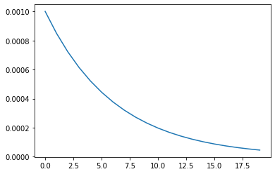
In the example above you can see that the learning rate gradually drops after each epoch. The initial learning rate is set to 0.001, and after 20 epochs the value dropped to 0.00001.
2. MultiplicativeLR
This method sets the learning rate of each parameter group to the learning rate in the previous epoch that is multiplied by a specified function. In the following example, the function is equal to the factor of 0.85 on the power of the epoch.
optimizer = torch.optim.SGD(model.parameters(), lr=0.001)
lam = lambda epoch: 0.85 ** epoch
scheduler = torch.optim.lr_scheduler.MultiplicativeLR(optimizer, lr_lambda=lam)
lrs = []

for i in range(20):
    optimizer.step()
    lrs.append(optimizer.param_groups[0]["lr"])
    print("Factor = ",0.85," , Learning Rate = ",optimizer.param_groups[0]["lr"])
    scheduler.step()

plt.plot(range(20),lrs)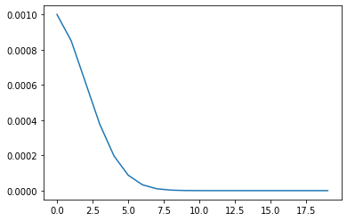
As you can see, this method is very similar to the previous one, only in this method, the learning rate drops at a faster rate.
3. StepLR
If you do not want your learning rate to decrease constantly you can apply a method called stepLR. This method decays the learning rate of each parameter group by the value of gamma every step_size epochs. In our example step_size is set to 5. That means that the initial learning rate will drop every 5 epochs by the value of gamma.
model = torch.nn.Linear(2, 1)
optimizer = torch.optim.SGD(model.parameters(), lr=0.001)
scheduler = torch.optim.lr_scheduler.StepLR(optimizer, step_size= 5, gamma=0.1)
lrs = []

for i in range(20):
    optimizer.step()
    lrs.append(optimizer.param_groups[0]["lr"])
    print("Factor = ",0.1 if i!=0 and i%2!=0 else 1," , Learning Rate = ",optimizer.param_groups[0]["lr"])
    scheduler.step()

plt.plot(range(20),lrs)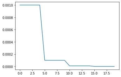
We have described some of the most popular methods for scheduling the learning rate. If you want to learn about other learning rate scheduling examples, check out this link.
3. Data augmentation
Training neural networks can be problematic especially if we don’t have a sufficient number of data in our dataset. One of the most popular methods that you can use to solve this problem and improve the performance of the model is called Data augmentation. It is a technique used to increase the amount of data by adding slightly modified copies of already existing data.
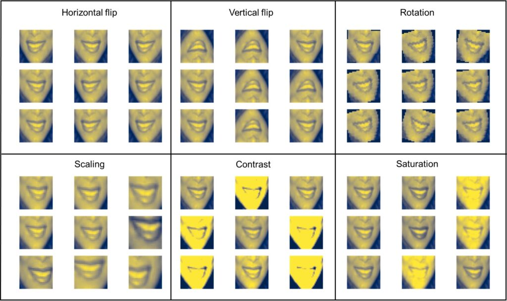
So, to get more data, we just need to make minor alterations to our existing dataset. Even though the changes that we are making are quite subtle, our neural network will think these are distinct images. In that way, we can double or triple the number of images in the dataset. The most common Data Augmentation techniques are:
- Translation
- Horizontal flip
- Vertical flip
- Rotation
- Scaling
- Cropping
- Adding a noise
- Brightness
- Contrast
- Color Augmentation
- Saturation
Let’s have a look at the following image and visualize some of the most popular Data augmentation methods.
Data augmentation in PyTorch
Applying data augmentation in Pytorch is very easy. We will just use torchvision.transforms and function transforms.Compose(). In our example, we are going to horizontally flip the images and apply a rotation of 5 degrees. and -5 degrees.
transform = transforms.Compose([
          transforms.Resize((32, 32)),
          transforms.RandomHorizontalFlip(),
          transforms.RandomRotation(degrees=(-5,5)),
          transforms.ToTensor()
          ])
Now, let’s visualize our transformations. In order to do this, we will pick one image from the train_data Then, we will iterate through the data and perform augmentation.
augmented_images = [train_set[5][0][0] for i in range(9)]
plt.figure(figsize=(8, 6))

for i in range(9):
  plt.subplot(3, 3, i+1)
  plt.imshow(augmented_images[i], cmap='cividis')
  plt.axis('off')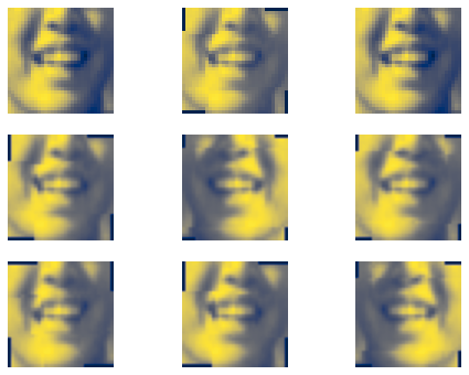
After applying data augmentation we are ready to train our model. The training process is the same as usual, and we will not get into deep details here. We are going to iterate through all training images and set them to work with the device we specified in the beginning. After that, we will set the gradients to zero, apply the forward propagation, calculate the loss and do the backpropagation step. After the training step, we will do the validation step as usual. We will iterate through all the validation images and use our model for predictions.
epochs = 50
train_loss = []
val_loss = []
t_accuracy_gain = []
accuracy_gain = []

for epoch in range(epochs):

    total_train_loss = 0
    total_val_loss = 0

    model.train()
    total_t = 0
    # training our model
    for idx, (image, label) in enumerate(trainLoader):

        image, label = image.to(device), label.to(device)
        optimizer.zero_grad()
        pred_t = model(image)

        loss = criterion(pred_t, label)
        total_train_loss += loss.item()

        loss.backward()
        optimizer.step()

        pred_t = torch.nn.functional.softmax(pred_t, dim=1)
        for i, p in enumerate(pred_t):
            if label[i] == torch.max(p.data, 0)[1]:
                total_t = total_t + 1

    accuracy_t = total_t / train_data_size
    t_accuracy_gain.append(accuracy_t)


    total_train_loss = total_train_loss / (idx + 1)
    train_loss.append(total_train_loss)

    # validating our model
    model.eval()
    total = 0
    for idx, (image, label) in enumerate(valLoader):
        image, label = image.to(device), label.to(device)
        pred = model(image)
        loss = criterion(pred, label)
        total_val_loss += loss.item()

        pred = torch.nn.functional.softmax(pred, dim=1)
        for i, p in enumerate(pred):
            if label[i] == torch.max(p.data, 0)[1]:
                total = total + 1

    accuracy = total / test_data_size
    accuracy_gain.append(accuracy)

    total_val_loss = total_val_loss / (idx + 1)
    val_loss.append(total_val_loss)

    if epoch % 5 == 0:
      print('\nEpoch: {}/{}, Train Loss: {:.4f}, Val Loss: {:.4f}, Val Acc: {:.4f}'.format(epoch, epochs, total_train_loss, total_val_loss, accuracy))
Now, let’s plot our training and validation loss and training and validation accuracy.
plt.plot(train_loss, "b", label="training_l")
plt.plot(val_loss, "r", label="validation_l")
plt.legend()
plt.plot(t_accuracy_gain, "b", label="training_accuracy")
plt.plot(accuracy_gain, "r", label="validation_accuracy")
plt.legend()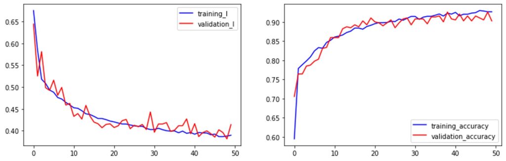
As you can see, we reached the validation accuracy of almost 92% which is a pretty good result. Note, that the training accuracy is going to increase if we continue training for more epochs. On the other hand, the test accuracy is going to level up at some point. This could be a good indication of how many epochs we should use for training this dataset. epochs.
The next step is to test our model. First, we are going to iterate through the test loader.
testiter = iter(testLoader)
images, labels = testiter.next()
Next, we need to turn off the gradient calculation using the function torch.no_grad(). Then, we will send our images and labels to the device. After that, we will create a prediction variable that will be equal to our trained model and images in the testLoader.
with torch.no_grad():
  images, labels = images.to(device), labels.to(device)
  pred = model(images)

images_np = [i.cpu() for i in images]
class_names = ['no_smile', 'smile']
Using the following code we can visualize the performance of our model. We will iterate through 50 images and plot them with their corresponding label. We will color the label in blue in case that our model predicted correctly, and in red if it failed to predict that class.
fig = plt.figure(figsize=(15, 7))
fig.subplots_adjust(left=0, right=1, bottom=0, top=1, hspace=0.05, wspace=0.05)

for i in range(50):
    ax = fig.add_subplot(5, 10, i + 1, xticks=[], yticks=[])
    ax.imshow(images_np[i].permute(1, 2, 0), cmap=plt.cm.gray_r, interpolation='nearest')

    if labels[i] == torch.max(pred[i], 0)[1]:
      ax.text(0, 3, class_names[torch.max(pred[i], 0)[1]], color='blue')
    else:
      ax.text(0, 3, class_names[torch.max(pred[i], 0)[1]], color='red')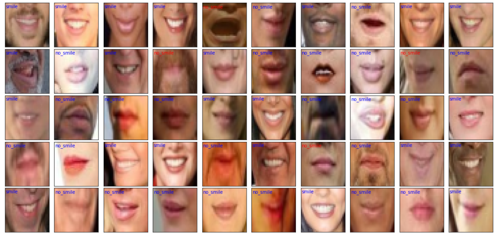
As you can see after training for only 50 epochs only 4 out of the 50 images were classified incorrectly. So we can say that Transfer learning, Data augmentation, and learning rate schedule significantly improved our model.
Summary
In this post, we have learned how to use various techniques in order to improve the pre-trained neural network. We have learned how to apply transfer learning, data augmentation, and how to schedule the learning rate. Combining these methods we were able to improve the performance of our smile detector and achieve accuracy close to 90%.