#007 How to implement GAN Hacks to Train Stable Models?

Highlights: In this post, we are going to learn several hacks that we can use to train stable GAN models. First, we are going to provide a quick recap of the GANs theory, and then, we are going to talk about challenges when training GANs. After that, we will provide solutions for these challenges in Python. So, let’s begin with our post.

Tutorial Overview:

Challenges when training GANs
Heuristics for Training Stable GANs
Architecture for guidelines for stable DCGANs

1. Challenges when training GANs

Training Generative Adversarial Networks (GANs), can be quite a challenging task. This is mainly because two networks, discriminator and generator, have to be trained simultaneously. This is done in the so-called min-max game. Due to this, when one model improves, it degrades the performance of the other and vice versa. Hence, the result is a very unstable training process. Moreover, this training process can also fail. For instance, a generator may be located at a point where it generates the same images all the time or that the images do not represent the dataset at all.

Therefore, scientists put a lot of hard work into experimenting and training GANs. Still, there is not much theoretical foundation, but the best practices for GAN training can be summarized in form of “Hacks”. Hence, in this post, we will review the most important hacks that have been introduced. Note, that most likely they offer an alternative way to create a neural network architecture and training process as compared to the standard design in the classification tasks of Computer Vision.

Therefore, this post will be, mainly hack-oriented, and thus, theoretical. Nevertheless, we will implement all the hacks, so they will be very handy for future off-the-shelf use in your projects. Last but not least, this post is mainly based on the fundamental overview and systematization of the GAN training recipes. These recipes are summarized in the 2015 paper by Alec Radford, et al. “Unsupervised Representation Learning with Deep Convolutional Generative Adversarial Networks”[1].

Commonly, this work is known as DCGAN. Please note that it can be confusing with conditional GANs. Hence, in the term DCGAN, the letters “DC” refer to Deep Convolutional architectures.

Finding the point of equilibrium

In the beginning, we have already stated that the inherent challenge in training GANs comes from the fact that there are two deep neural networks being trained simultaneously. Thus, this competing game should hopefully end in finding the point of equilibrium. This is the so-called Nash equilibrium of a two-player non-cooperative game. However, reaching this point is very difficult. Mostly, the optimization functions are non-convex, the parameters are continuous and the parameters space is extremely highly-dimensional [2].

Moreover, due to constant changes in the model and the parameters, the nature of the optimization problem is continually changed. Hence, we practically obtain a dynamic system where the optimization process does not seek a minimum, but an equilibrium between two opposing forces.

On the other hand, when we were training neural networks for classification, it rarely happened that the network would be stuck. Although, we did know that we are not reaching a global minimum. However, the network would still produce satisfying results and we would not consider training in more depth. In contrast to this, GANs can fail to converge. For example, instead of finding a point of equilibrium, it would oscillate between generating specific examples in the domain. The failure model can be such that in the case of multiple inputs to the generator, the output is always the same. In other words, for the different latent vectors $z $ (input to generator) the network would produce the same result. Hence, this is known as a mode collapse. As such, it potentially represents one of the most challenging failures while training GANs.

Evaluate the success of training GANs

Last but not least, it is the challenge to objectively evaluate the success of training GANs. This is a particular challenge during the training itself as there is a lack of an objective metric for this task. For instance, if we are generating synthetic faces, it is not easy to come up with an effective metric to describe the quality. In this, as in many other cases of image synthesis, visual inspection represents by far the most effective way to evaluate the quality.

2. Heuristics for Training Stable GANs

Deep Convolutional GANs (DCGANs)

After the publication of the original GAN paper in 2014, there were many questions with respect to training GANs efficiently. The first pioneering work that exhaustively reviewed numerous experimental and theoretical approaches was done by Radford et al. [1]. There, the researchers proposed several important recipes or “hacks” that were confirmed in practice to produce good results. All this was done with the goal to improve the stabilization of GANs and optimizing the GAN model architectures as well as hyperparameters.

This work is referred to as Deep Convolutional Generative Adversarial Networks or DCGANs. Naturally, this network does not have fully connected layers and the originally proposed architecture is shown in the image below:

As such, this remains a highly recommended starting point when developing a new image synthesis task, at least when the image synthesis is concerned. The authors proposed that after extensive model exploration they were able to identify a family of architectures that results in a stable training process across a range of datasets and allowed for training higher resolutions and deeper generative models. The following paragraph is a brief summary of the recommendations.

3. Architecture for guidelines for stable DCGANs

In this part, we review the main hacks that are proposed in the scientific community. First, we briefly explain the use and the motivation for the hack. Then, we show in a code snippet how it can actually be implemented using PyTorch.

Here, we can see the architecture for the stable DCGANs

Replace every pooling layer with a Strided Convolution in the discriminator and Fractional-Strided Convolutions in the generator.
Use the batch normalization method in both the generator and the discriminator.
Remove fully connected hidden layers for deeper architectures.
Use the ReLU activation function for all layers except for the output. For the output later use the Tanh function.
Use the ReLU activation function in the discriminator for all layers.

Downsampling using Strided Convolutions

The discriminator is a standard neural network and in GANs for image generation, its input is an image. This image is passed forward through the network and processed with layers. Notably, the layer will shrink the size of the input image and this is commonly done in the max polling part. However, this process can be achieved also within a standard convolutional layer in case we increase the stride.

Commonly, the stride is set to $(1,1) $ when working with convolutional layers. However, if we set it to $(2,2) $ we will produce an effect of convolution while downsampling the input image (or feature map) by a factor of two. That is, the input image will be one-quarter of the original input image.

In the DCGAN paper, the authors advocate the use of standard convolution with a stride of $(2,2) $ for downsampling. This is referred to as strided convolution. For instance, an image of size $64\times64 $ will be downsampled to size $32\times32 $.

In PyTorch this can be implemented fairly easily. We will just use the standard convolutional layer and as the parameter, for the stride, we will use the input parameters $(2,2) $. So, that’s all and it can be achieved with the following code.

import torch 
import torch.nn as nn

class Downsample1(nn.Module):
    def __init__(self):
        super(Downsample1, self).__init__()
        self.Down = nn.Conv2d(3, 1, kernel_size=(3,3), stride=(2,2), bias = False)
 
    def forward(self, x):
        x = self.Down(x)
        return x

test_image = torch.rand( 3,28,28)
test_image = test_image.unsqueeze(0)

Down = Downsample1()
output = Down(test_image)

#test_image.shape
output.shape

Output:

torch.Size([1, 1, 13, 13])

Upsampllening Using Strided Convolutions

In GANs, we have two neural networks that perform different tasks. First, the discriminator is classifying an input image $x $ (very high-dimensional input), to produce a single scalar output value. Hence, in this process, we mainly have the process of downsampling. On the other hand, the generator receives at its input a latent vector $z $ (much lower dimension than $x $), and from this vector $z $, it should generate an output image $x $. Hence, in this case, we have a network with the goal to increase the dimensionality and add new information to our final generated image ($x $). For this, we can use a simple upsampling operator. In addition, the upsampling can be achieved using for instance bilinear interpolation. On the other hand, it can be done with the convolutional layer. In this case, we use a transposed convolution (also referred to as dilated convolution). The following image illustrates the process of transpose convolution.

We will zero pad the original image, $3\times3 $, and place the paddings on all sides of the pixels. These are represented as white squares. This way we went from the original $3\times3 $ image to a $7\times7 $ image that is zero-padded image.
Then, we will have a $3\times3 $ convolution filter (kernel) that we will use to produce our output. Note that this filter is shown as a gray square ($3\times3 $) that is moving across the image.
By moving the kernel, we can see that at that particular position, it will generate one output element (pixel) of the output feature map on the top ($5\times5 $).

To can implement transpose convolution in Pytorch, we just need to apply the function nn.ConvTranspose2d() instead of the function nn.Conc2d().

class Upsample(nn.Module):
    def __init__(self):
        super(Upsample, self).__init__()
        self.Up = nn.ConvTranspose2d(3, 1, (3,3), (2,2))        

    def forward(self, x):
        x = self.Up(x)
        return x

image = torch.rand((3, 256,256)) * 255
image = torch.tensor(image)
image = image.unsqueeze(0)

image.shape

Output:

torch.Size([1, 3, 256, 256])

Up = Upsample()
image2 = Up(image)
image2.shape

Output:

torch.Size([1, 1, 513, 513])

Use Leaky ReLU

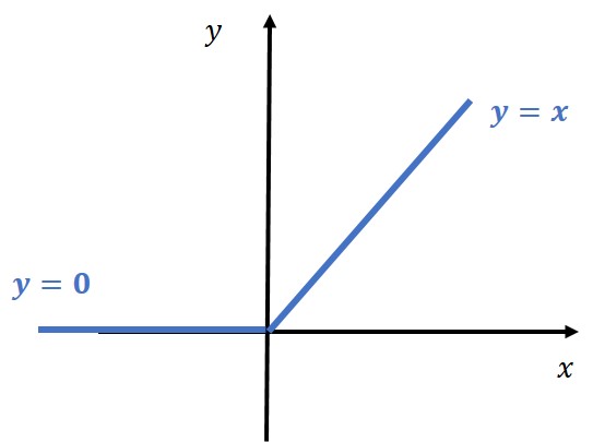
In standard convolutional networks, we have witnessed a breakthrough in the past several years. One of the novelties that contributed to this progress is the use of the ReLU – Rectified Linear Unit activation function. Mathematically, it is defined as :

$$ y =max(0,x) $$

To visualize the ReLU function take a look at the following image

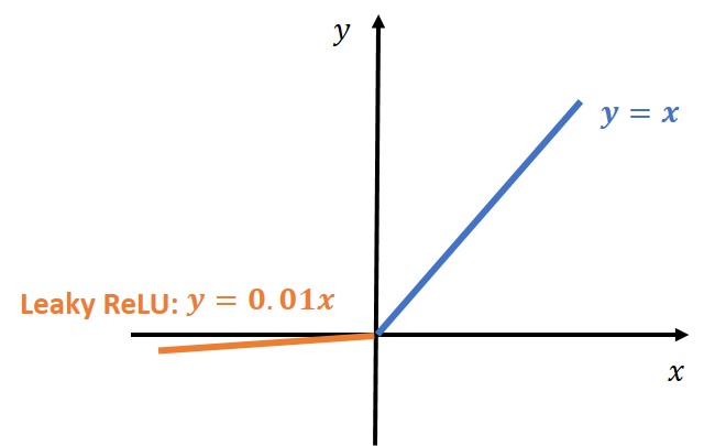
However, when working with GANs it was revealed that a variant of ReLU, known as LeakyReLU would give better performance and more stable training.

Leaky ReLU has a small slope for negative values, instead of altogether zero. For example, leaky ReLU may have $y = 0.01x $ when $x<0 $.

Parametric ReLU (PReLU) is a type of leaky ReLU that, instead of having a predetermined slope like 0.01, makes it a parameter for the neural network to figure out itself when $x<0 $:

$$ y = ax $$

We can see that the difference is that we have a negative slope and not a zero value for the negative input $x $. It is recommended that a value of 0.2 can be used. Initially, the use of ReLU was recommended for the discriminator. However, it is a safe practice today to be used in both discriminator and generator.

class Downsample2(nn.Module):
    def __init__(self):
        super(Downsample2, self).__init__()
        self.Down = nn.Conv2d(3, 1, kernel_size=(3,3), stride=(2,2), bias = False)
 
        # 3. this part is simple, we have just to add a LeakyReLU activation function
        # and to define its slope
        self.leaky = nn.LeakyReLU(0.2)
 
    def forward(self, x):
        x = self.Down(x)
        x = self.leaky(x)
        return x


test_image = torch.rand( 3,28,28)
test_image = test_image.unsqueeze(0)

Down = Downsample2()
output = Down(test_image)

#test_image.shape
output.shape

Output:

torch.Size([1, 1, 13, 13])

Use Batch Normalization

A layer, known as Batch Normalization, standardizes the outputs from the previous layer. This is done in such a way that the further signal is passed and has zero mean value and a unit standard deviation.

The use of Batch Normalization in code is rather straightforward. We just need to add a single function as a layer as can be seen in the following code snippet.

class Downsample3(nn.Module):
    def __init__(self):
        super(Downsample3, self).__init__()
        self.Down = nn.Conv2d(3, 1, kernel_size=(3,3), stride=(2,2), bias = False)
        # this is the only line that we have added
        # the use of batch normalization
        torch.nn.init.normal_(self.Down.weight)
        self.batch = nn.BatchNorm2d(1)
        self.leaky = nn.LeakyReLU(0.2)
 
    def forward(self, x):
        x = self.Down(x)
        x = self.batch(x)
        x = self.leaky(x)
        return x

test_image = torch.rand( 3,28,28)
test_image = test_image.unsqueeze(0)

Down = Downsample4()
output = Down(test_image)
output.shape

Output:

torch.Size([1, 1, 13, 13])

Use Gaussian Weight Initialization

When working with generators and discriminators we will need to initialize the weights. So far, you have probably encountered some of the popular initialization methods, such as Xavier or He. In GANs, a simple Gaussian weight initialization is recommended. Moreover, it is recommended to set a mean value to 0, while the standard deviation should be set to 0.02. This also can be implemented in an easy way.

def init_normal(m):
    if type(m) == nn.Conv2d:
        nn.init.uniform_(m.weight, 0, 0.02)
 
# use the modules apply function to recursively apply the initialization
Down.apply(init_normal)

Use Adam optimization algorithm

Next, as optimization is concerned we have explored various options for the Convolutional Networks. For GANs, similarly, as for the Convolutional Networks, the Adam optimization algorithm is recommended. Here, we defined how an optimizer variable can be initialized with Adam. The model parameters are passed as inputs:

# Use Adam optimization algorithm
optimizer = torch.optim.Adam(Down.parameters(), lr=0.0002)

Use rescaled images on the interval $[-1, 1] $.

In DCGAN work, a hyperbolic tangent function has been recommended for the generator. Hence, the real images that we use in the discriminator are also rescaled to the interval of $[-1, 1] $. Commonly, we have images that are encoded as unsigned integers, thereby being in the interval from $[0, 255] $. The following simple function can be used to rescale all the data so that we have a standardized input into the discriminator:

# Scale images to the interval [-1,1]
 
image = torch.rand((3, 100,100))
image = image * 255
image = image.to(torch.uint8)

def rescale_image(image):
    image = image - 127.5 
    image = image / 127.5
    return image

rescale_image(image)

Well, this concludes all the hacks! I hope that you have enjoyed them as presented by a dataHacker team 🙂

Keep hacking!

In future posts, we will start implementing more advanced networks and models.

Summary

When they appeared for the first time a huge GAN potential was immediately realized. However, the first network was only able to work on relatively simple datasets, and as such their early applicability was limited. Mainly, this was the case as the training was inherently dynamic and represented quite an unstable process. Many experiments with or without strict theoretical background were conducted. Hence, this resulted in a set of hacks that we have presented here. In this chapter, we have mainly used the hacks as presented in the paper that is known as DCGAN (2015.).

References:

[1] Radford, Alec, Luke Metz, and Soumith Chintala. “Unsupervised representation learning with deep convolutional generative adversarial networks.” arXiv preprint arXiv:1511.06434 (2015).

[2] Salimans, Tim, et al. “Improved techniques for training GANs” Advances in neural information processing systems 29 (2016): 2234-2242.

2015 paper by Alec Radford, et al. “Unsupervised Representation Learning with Deep Convolutional Generative Adversarial Networks”

#007 How to implement GAN Hacks to Train Stable Models?