#006 GANs - How to Develop a 1D GAN from Scratch

#006 GANs – How to Develop a 1D GAN from Scratch

Highlight: In this post, we will briefly review the theory behind Generative Adversarial Networks and then we will learn to implement that knowledge in PyTorch. We will actually build our first GAN from scratch so that all the details are demystified. Initially, we will start with generator modeling or faking a simple 1D function (sine wave). In the later posts, we will build on the fundamental GAN architecture presented in this post.

Tutorial Overview:

GAN theory – quick recap
A 1D function that we want to model – a sine wave
Define a Discriminator Model
Training a discriminator
Define a Generator Model
Generating fake data
GAN training

1. GANs theory – a quick recap

So far we have introduced and reviewed theories related to GANs. That is, we gave an intuitive overview of this new and modern family of deep learning architectures. Let us repeat that in GAN we have two (deep) neural networks called Generator and Discriminator.

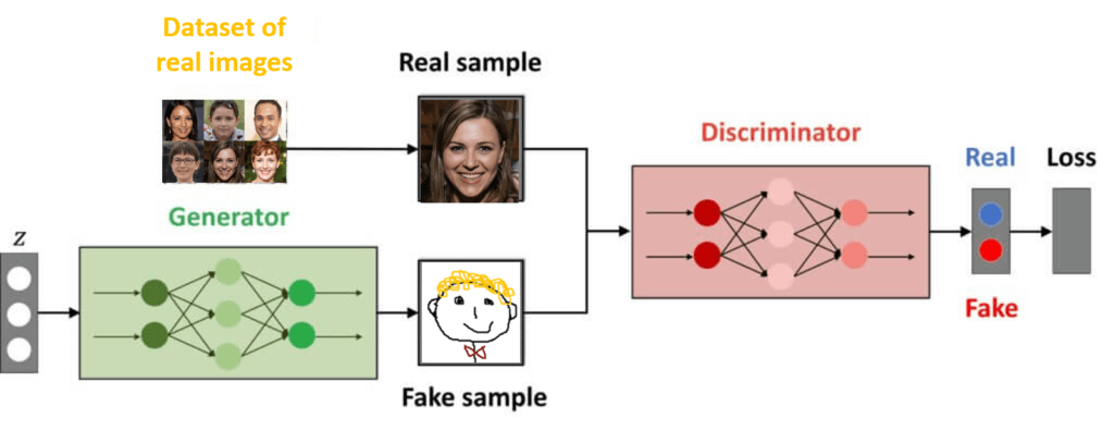
In addition, we work with real data samples and we say that they represent “real data”. The goal of the generator (deep neural network) is to try to replicate samples from this dataset and to create new, so far, unseen images. To succeed in this, we also introduce a discriminator. It is a neural network as well and jointly with the generator it will play the minimax optimization game.

The goal of this game is to simultaneously improve both the discriminator and the generator. On the other hand, although this idea is quite appealing, now the challenge can be to fully understand all the details. I had the same feeling when I first saw GAN examples. However, do not worry! We will start this chapter with practical implementation in PyTorch. Our first model will be very simple. We will develop a GAN that should generate numbers according to a 1D function.

2. A 1D function that we want to model – a sine wave

First, we will start with modeling the 1D function. Here, we will work with a sine wave function. We will model the so-called, one period or one cycle of this function.

$$ f(x) = sin( 2 \cdot \pi \cdot x) $$

Here, we will assume that the $x $ represents a random variable that follows a uniform distribution defined on the interval $[0, 1] $. This is easy to program in PyTorch. We will work with PyTorch instead of NumPy just to practice the use of tensors.

First, let’s import the necessary libraries.

import torch 
import torch.nn as nn
import matplotlib.pyplot as pltCode language: JavaScript (javascript)

Next, we define a simple 1D function that we want to model with GANs. The (input, output) relation that is $(x, sine(x)) $ will be joined and used as an input to a discriminator. If the pair follows a sine function it will be regarded as a true data label. Otherwise, it will be judged as a fake data point. Then, the generator will try to learn this mapping and fool a discriminator.

def sine_function(x):
    return torch.sin(x)

# test sine_function()    
print(sine_function(torch.tensor(torch.pi * 0.5 )))
print(sine_function(torch.tensor(torch.pi * 0. )))Code language: CSS (css)

Output:

tensor(1.)
tensor(0.)

In the following block, we have defined the sine wave as applied directly on $x $. However, note that when we create a dataset, we will multiply the $x $ with $2 \cdot \pi $.

x = torch.rand(100) * 2 * torch.pi
y = sine_function(x)
# plot the sine wave function
plt.scatter(x.numpy(), y.numpy())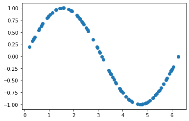Code language: PHP (php)

We can see what our distribution looks like. Along the horizontal axis we have $x $, and along the vertical axis we have $sin( 2 \cdot \pi \cdot x) $ values plotted.

Well, you may ask yourself. What is now going to be our $x $ that we used to denote images? Only the $sin( 2 \cdot \pi \cdot x) $ values ? Are we interested in learning how to generate these?

Well, not exactly. Here, we need to learn the complete mapping process, so that we have an effective generator. That is, we will treat the input-output pair, as the desired output of the generator that we want to design. Hence, the dataset will be in form ($x $ , $sin(2\cdot \pi\cdot x ) $ ). That is, the output of the generator we expect to obey a similar behavior. It will output two elements, where the second one is dependent on the first element.

Generate data samples

The following code snippet will assist us to generate data samples. In practice, they will come from the real dataset. For instance, we can use the face images of famous actors.

def generate_data_samples(n=100):
    # here we define the number of n numbers from a Uniform distribution
    x1 = torch.rand(n) * 2 * torch.pi
    x2 = sine_function(x1)
    x1 = x1.view(n,1)
    x2 = x2.view(n,1)
    y_data = torch.ones((n,1))

    return torch.hstack((x1, x2)), y_dataCode language: PHP (php)

The function returns the data pair as well as the label. Here, we will return the variable y_data, that will be set to 1, as expected for the real data samples.

test_generated_data = generate_data_samples(100)

plt.scatter(test_generated_data[0][:,0].numpy(), test_generated_data[0][:,1].numpy())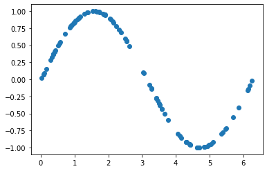

So, to model this data relation, we will develop a generator. We will start with a very simple model. We will assume that it is a neural network with a very simple architecture that has only fully-connected layers. For such a network we will provide a randomly generated input $z $ (latent space variable) and for this example, we will choose that the dimension of the $z $ vector is equal to 5.

That means that we want to develop a generator whose input is a random vector of 5 elements. At the output, we want to get two elements, where the second one models the function $sin(2\cdot \pi\cdot x ) $. In addition, the interval for the first element should match the interval from which the real data is generated. In our case, since $x $ is a uniform random variable from an interval $[0,1] $, the first element of the generator will actually be $[0, 2\cdot \pi] $.

Before we proceed further with the generator, let’s discuss the use of the discriminator. This will also be a simple neural network. Its input vector will obviously be of size 2. The input vectors can come from the real data or from the fake generated dataset using a generator model. The role of the discriminator is to accurately distinguish between the real data (class=1) and the fake data (class=0)

3. Define a discriminator model

Here, we will define a discriminator model and since we are learning a simple distribution we can start off with a simple neural network. An input to this network will be a 2-dimensional vector that has the structure ($x $ , $sin(2\cdot \pi\cdot x ) $ ).

The goal of the discriminator is to distinguish between the real and fake data samples. Since this is an introductory example, we also generate the real data, via our function defined in the previous paragraph.

Here, we will also introduce a function that will generate “dummy” fake data. Note that this function will help us to understand all the details step by step and not rush to work with the generator. Hence, we will design a function to output a pair of numbers that will be completely random. This dataset will not be changed or updated as in the case when we work with the generator model in parallel as well.

To achieve this, we will define the discriminator network with simple output. This is because it will represent a simple binary classification problem.

For the loss function, we will select a binary cross-entropy function. The network will be trained using both real and dummy-fake generated data.

We will start with the implementation of the discriminator. Note, that this is the first model that we are building in PyTorch and therefore it will be relatively easy and straightforward.

In case you need a refresher about your PyTorch knowledge we have the complete series on our blog datahacker.rs.

The following code snippet demonstrates how we can implement a simple discriminator. Here, the input size is 2, whereas the output is set to 2 as well. In the middle, we have selected only one hidden layer of size 25.

class Discriminator(nn.Module):
    def __init__(self):
        super(Discriminator, self).__init__()
        self.fc1 = nn.Linear(2, 25)
        self.fc2 = nn.Linear(25,1)

    def forward(self,x):
        x = self.fc1(x)
        x = F.relu(x)
        x = self.fc2(x)
        x = torch.sigmoid(x)
        return x

The first part or __init__() function defines two layers: fc1 and fc2 (fully connected 1 and 2). As for the activation function in the hidden layer, we will use a ReLU. For the output layer, we will naturally select a sigmoid function.

This defines the discriminator class. It is convenient at this stage to do a sanity check. As an input to a discriminator model, we can simply use a two-element random vector, to validate our implementation

discriminator = Discriminator()
# test a discriminator with a simple input - sanity check
x_data_test = torch.rand(2)
discriminator(x_data_test)Code language: PHP (php)

Output:

tensor([0.4532], grad_fn=<SigmoidBackward0>)Code language: HTML, XML (xml)

As you can see we didn’t get any errors, and therefore, as far as the syntax is concerned and dimension matching we have done a good job. We can now proceed.

Next, in a step-by-step fashion, while keeping our focus on the discriminator we will need to design a training mechanism for the discriminator. To do this, we will generate a dummy-fake dataset. For this, we will use a simple idea that the two random variables will constitute an input pair that the discriminator has to distinguish. Naturally, this will be a very easy task for our discriminator.

def generate_dummy_fake_data(n):
    x1 = torch.rand(n) * 2 * torch.pi
    x2 = torch.rand(n) * 2 * torch.pi
    x1 = x1.view(n,1)
    x2 = x2.view(n,1)
    y_fake = torch.zeros((n,1))
    return torch.hstack((x1, x2)), y_fakeCode language: JavaScript (javascript)

Now, let’s plot the fake data.

x_fake,y_fake = generate_dummy_fake_data(100)
plt.scatter(x_fake[:, 0].numpy(),x_fake[:, 1].numpy())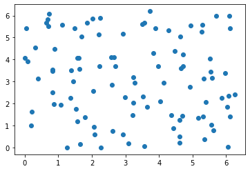

4. Training a discriminator

In this part, we will implement a standard PyTorch framework for the training of neural networks. It is a simple exercise and it can serve as a PyTorch and Deep Learning refreshing paragraph.

We will start with the standard definition of the parameters and choose the desired algorithms.

discriminator = Discriminator()
optimizer = torch.optim.Adam(discriminator.parameters(), lr = 0.001) 
criterion = torch.nn.BCELoss()

Here, we can define an arbitrary number of epochs=1000.

Next, we can define the batch size. Here, it is specified with a variable n. In essence, it tells us how many samples from the real data and dummy-fake dataset we want to generate. Here, we have set it to 100.

epochs = 1000
n = 100
x_data, y_data = generate_data_samples(n)
x_fake, y_fake = generate_dummy_fake_data(n)

x_all = torch.vstack((x_data, x_fake))
y_all = torch.vstack((y_data, y_fake))
all_loss = []
for i in range(epochs):
    y_hat = discriminator(x_all)
    loss = criterion(y_hat, y_all)
    all_loss.append(loss.item())

    loss.backward()
    optimizer.step()
    optimizer.zero_grad()

The remainder of the code concatenates both real (class=1) and fake (class=0) data into a single variable, as well as their labels in a consistent way. Here, we can see that the loss function is decreasing rapidly, thereby suggesting that this classification task is easy for the discriminator.

plt.plot(all_loss)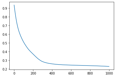Code language: CSS (css)

5. Define a generator model

In most of the cases, at least in the introductory GAN architectures, it does make sense to observe the generator/discriminator network in the sense of the decoder/encoder structure. In this way, we can assume that the architecture of the generator should be somehow symmetrical as compared with the discriminator, at least to a certain degree.

The following code snippet will show how we can implement a generator. Here, we again use a very simple and shallow neural network.

# define a Generator Model

class Generator(nn.Module):
    def __init__(self):
        super(Generator, self).__init__()

        self.fc1 = nn.Linear(5,15)
        self.fc2 = nn.Linear(15, 2)

    def forward(self, x):
        x = self.fc1(x)
        x = F.relu(x)
        x = self.fc2(x)
        # note that here we are not adding any activation functions
        # since we assume the linear output as the values can be negative as well
        # in other words this activation function here is just an "identity function" f(x)=x
        return x

We need to define a hidden layer with 15 neurons. It is processing a data vector from the input of the neural network of size 5. Here, we have opted for an ReLU activation function. For the output layer, we select two neurons and these two neurons should output and learn to model our desired distribution pair ($x $ , $sin(2\cdot \pi\cdot x ) $ ). Hence, we can have negative values as well. Here, we will then skip defining the activation function. We will just use a linear function that creates a fully connected layer (fc2). We can also assume that the activation function is an identity function ($f(x)=x $).

Inputs: Points in a latent space e.g., a five-element vector of Gaussian random numbers
Outputs: Two=element vector representing a generated sample for our function

Here is a sanity check for the generator. Just to make sure that our neural network is correctly implemented.

generator = Generator()
test_generator = generator(torch.rand(5))
print(test_generator)Code language: PHP (php)

Output:

tensor([ 0.1416, -0.1184], grad_fn=<AddBackward0>)
Code language: HTML, XML (xml)

We see that it outputs a vector with two elements. Since the current weights are randomly initialized, we do not expect any meaningful result at the output so far. We still need to reach the GAN training phase for this.

6. Generating fake data

As the next step, we need to see how to create fake data. For this, we will use the following. As input, we will have our initial latent vector $z $ of dimension 5. Then, this vector will be used as the input to the generator which will output a two-element vector. In addition, we usually want to create a full batch of such data samples and we will do this within the following function:

def generate_latent_points(n, latent_dim=5):
    # here we will assume that in the z-space 
    # or latent space we have 5 dimensional random vector 
    z = torch.rand(n*latent_dim)
    return z.view((n,latent_dim))

a = generate_latent_points(10)
print(a)Code language: PHP (php)

Output:

tensor([[0.5269, 0.7959, 0.9375, 0.5916, 0.1423],
        [0.7983, 0.5828, 0.5751, 0.4969, 0.0013],
        [0.0949, 0.9805, 0.3409, 0.1454, 0.6456],
        [0.3170, 0.0603, 0.8505, 0.9386, 0.1067],
        [0.3837, 0.9221, 0.2591, 0.3959, 0.8892],
        [0.8514, 0.1856, 0.1732, 0.6434, 0.7440],
        [0.4870, 0.4249, 0.5836, 0.6097, 0.8979],
        [0.1552, 0.3635, 0.2549, 0.2609, 0.2949],
        [0.6123, 0.5833, 0.2193, 0.0419, 0.0678],
        [0.8755, 0.6912, 0.2100, 0.5914, 0.4561]])Code language: CSS (css)

As you can see, this data is structured as a matrix of size $n\times5 $. Next, this latent vector should be passed through the generator and this step will generate the fake data.

def generate_fake_samples(generator, n, latent_dim=5):
    z = generate_latent_points(n)
    fake_data = generator(z)
    return fake_data Code language: JavaScript (javascript)

fake_data_test = generate_fake_samples(generator, 100)
plt.scatter(fake_data_test[:,0].detach().numpy(), fake_data_test[:,1].detach().numpy())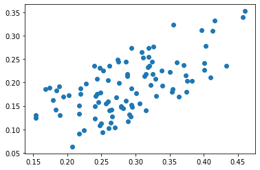

Here, we have plotted 100 elements from the fake data generated with the generator. In the image above you can see what our fake data do look like.

This dataset is created when the generator neural network is initialized with the random weight values. Once we start the GAN training minimax game, these values will be updated and the fake data will start to gradually resemble the original real data samples. Naturally, if the training proceeds according to the plan.

7. GAN training

In this part, we will see how we can simultaneously train both generator and discriminator. To remind ourselves:

The goal of the discriminator is to classify real from fake data
The goal of the generator is to generate realistic fake replicas from the original dataset

This algorithm can be implemented within a standard PyTorch framework. For this, we just need to define some parameters initially.

training_steps = 200000    

# Models
generator =     Generator()
discriminator = Discriminator()

# Optimizers
generator_optimizer     = torch.optim.Adam(generator.parameters(),     lr=0.001)
discriminator_optimizer = torch.optim.Adam(discriminator.parameters(), lr=0.001)

# loss
loss = nn.BCELoss()

N = 128

for i in range(training_steps):
    # zero the gradients on each iteration
    generator_optimizer.zero_grad()
    if i%5000 ==0:
        print(f"{i} \n")
    # Create a fake data with a generator
    fake_data = generate_fake_samples(generator, N)
    # here we define the INVERSE labels for fake data
    fake_data_label = torch.ones(N,1)
    # Generate examples of real data

    real_data, real_data_label = generate_data_samples(N)
    
    # Train the generator
    # We invert the labels here and don't train the discriminator because we want the generator
    # to make things the discriminator classifies as true.
    generator_discriminator_out = discriminator(fake_data)
    generator_loss = loss(generator_discriminator_out, fake_data_label)
    generator_loss.backward()
    generator_optimizer.step()Code language: PHP (php)

You may notice that the variable training_steps is set to a particularly large value for such simple networks. Welcome to GAN’s world! 🙂 The variable N will define the size of our two batches. Here, for each training iteration, we need to generate new data samples. We will “draw” them using two functions generate_fake_samples() and generate_data_samples() that we previously implemented

In addition, we will be careful to set the corresponding labels for these samples. So, the first important thing to specify is this. Please, make sure that you grasp this idea carefully. For the generator training, we will use fake data samples. However, we will set that these samples are coming from the “real dataset”. Thus, we will falsely assign that they are coming from class 1 (inverse labeling). We will explicitly define it with the command torch.ones().

Next, we will use these data samples as input to our discriminator. We want on purpose to generate a large error so that the update of the generator’s parameters takes place. In contrast, we can imagine that the discriminator would just correctly classify them as false. In this way, we will not be able to backpropagate the error signal that needs to update the parameters of the generator.

Training a discriminator

In the next phase, we need to update the discriminator. We will train it using both the fake and the real data. In this case, however, we want the fake data to belong to their class=0. There is no need to perform inverting here. Hence, we will use the class labels that are set to 0.

# Train the discriminator on the true/generated data
    discriminator_optimizer.zero_grad()
    true_discriminator_out = discriminator(real_data)
    true_discriminator_loss = loss(true_discriminator_out, real_data_label)

    # add .detach() here. Think about this
    # here a fake_data is passed with a gradient turned off
    # see our post about <a href="https://datahacker.rs/004-computational-graph-and-autograd-with-pytorch/#Automatic-differentiation-module-in-PyTorch---Autograd">AUTOGRAD</a>
    generator_discriminator_out = discriminator(fake_data.detach())
    generator_discriminator_loss = loss(generator_discriminator_out, torch.zeros(N,1))
    discriminator_loss = (true_discriminator_loss + generator_discriminator_loss) / 2
    discriminator_loss.backward()
    discriminator_optimizer.step()Code language: PHP (php)

Subsequently, we will perform the training using the real dataset whose class labels are set to 1. Note a few subtleties here. First of all, when we pass fake data samples to a discriminator we will use a function .detach(). In this way, we will turn off gradient calculations and this data will be treated as constant data values.

Next, note that we define the discriminator_loss as the mean value from both the real and fake data. We accomplish this with simple division by 2, but we have also to make sure that we have the same number of training samples (batch size) for both datasets.

We perform the optimization of the parameters with the standard .backward() and .step() methods. Believe it or not, we are ready. Here, we will show the GAN training part of the code for completeness.

training_steps = 200000    

# Models
generator =     Generator()
discriminator = Discriminator()

# Optimizers
generator_optimizer     = torch.optim.Adam(generator.parameters(),     lr=0.001)
discriminator_optimizer = torch.optim.Adam(discriminator.parameters(), lr=0.001)

# loss
loss = nn.BCELoss()

N = 128

for i in range(training_steps):
    # zero the gradients on each iteration
    generator_optimizer.zero_grad()
    if i%5000 ==0:
        print(f"{i} \n")

    # Create a fake data with a generator
    fake_data = generate_fake_samples(generator, N)

    # here we define the INVERSE labels for fake data
    fake_data_label = torch.ones(N,1)

    # Generate examples of real data
    real_data, real_data_label = generate_data_samples(N)
    
    # Train the generator
    # We invert the labels here and don't train the discriminator because we want the generator
    # to make things the discriminator classifies as true.
    generator_discriminator_out = discriminator(fake_data)
    generator_loss = loss(generator_discriminator_out, fake_data_label)
    generator_loss.backward()
    generator_optimizer.step()

    # Train the discriminator on the true/generated data
    discriminator_optimizer.zero_grad()
    true_discriminator_out = discriminator(real_data)
    true_discriminator_loss = loss(true_discriminator_out, real_data_label)

    # here a fake_data is passed with a gradient turned off
    # see our post about <a href="https://datahacker.rs/004-computational-graph-and-autograd-with-pytorch/#Automatic-differentiation-module-in-PyTorch---Autograd">AUTOGRAD</a>
    generator_discriminator_out = discriminator(fake_data.detach())
    generator_discriminator_loss = loss(generator_discriminator_out, torch.zeros(N,1))
    discriminator_loss = (true_discriminator_loss + generator_discriminator_loss) / 2
    discriminator_loss.backward()
    discriminator_optimizer.step()Code language: PHP (php)

Once we run we can already experience the inherent instability of the GAN networks. In our experiments, especially for a smaller number of training iterations (e.g. 10, 000), it can happen that we do not reach the convergence.

Hence, we have played around with the parameters until we managed to produce satisfying results. Here is one example of our experiments.

plt.scatter(real_data[:,0].detach().numpy(), real_data[:,1].detach().numpy())
plt.scatter(fake_data[:,0].detach().numpy(), fake_data[:,1].detach().numpy())Code language: CSS (css)

Once the training phase was over, we used the generator to create a new batch size for us. We have plotted this set (orange) along with the real data (blue). We can notice a few things. First, it makes sense to interpret this as a 2D probability distribution. Indeed, we have two variables, x1 and x2 that depend on each other. Next, we can notice one interesting thing and this is the relatively piece-wise linear part in the interval from 4 to 6. This can imply the complexity of the network and the underlying mechanism of how the data is actually being generated.

Finally, in the end, we compare and evaluate our results only visually.

In the next chapters, we will introduce objective measures to quantify the performance of the generator.

Congratulations! You have just mastered your first GAN network. In the next posts, we will explore more complex datasets, with more challenging probability distributions. In addition, we will learn a lot of tips and tricks on how to better train GANs.

Summary

As the introductory chapter for GAN’s implementation in PyTorch, we have opted to implement simple generator and discriminator architectures. We learned how to train them separately, how to generate latent data as well, and how to generate the fake dataset. In addition, we learned how a minimax game can be implemented in PyTorch. Finally, we showed very interesting artificially synthesized results and are ready to tackle more challenging and fascinating problems.

#006 GANs – How to Develop a 1D GAN from Scratch