LLM_log #010 Understanding Diffusion Models Through 1D Experiments — From DDPM to Manifold Compactness

Highlights:
We implement a complete DDPM from scratch on 1D sine waves — same math as image diffusion, but every intermediate state is plottable. We track 100 parallel trajectories, measure when the model “commits” to a specific sample, then design a controlled experiment that reveals manifold compactness as the key factor determining whether diffusion succeeds or fails. So let’s begin!
Tutorial Overview:
- Why 1D?
- The Dataset
- Forward Process
- Model and Training
- Generating from Noise
- What Does the Model Learn?
- 100 Parallel Trajectories
- When Does Diffusion Fail?
- Isolating the Variable
- Implications for Image Diffusion
1. Why 1D?
When training a diffusion model on 64×64×3 images, you can see the input and the output — but what about the 1,000 intermediate steps? When does the model “recognize” which image it is generating? You cannot answer this in 12,288 dimensions.
We replace images with 256-point sine waves. The DDPM math stays identical. The difference: we can now plot everything — overlay 100 trajectories, visualize convergence, measure the exact moment of commitment.
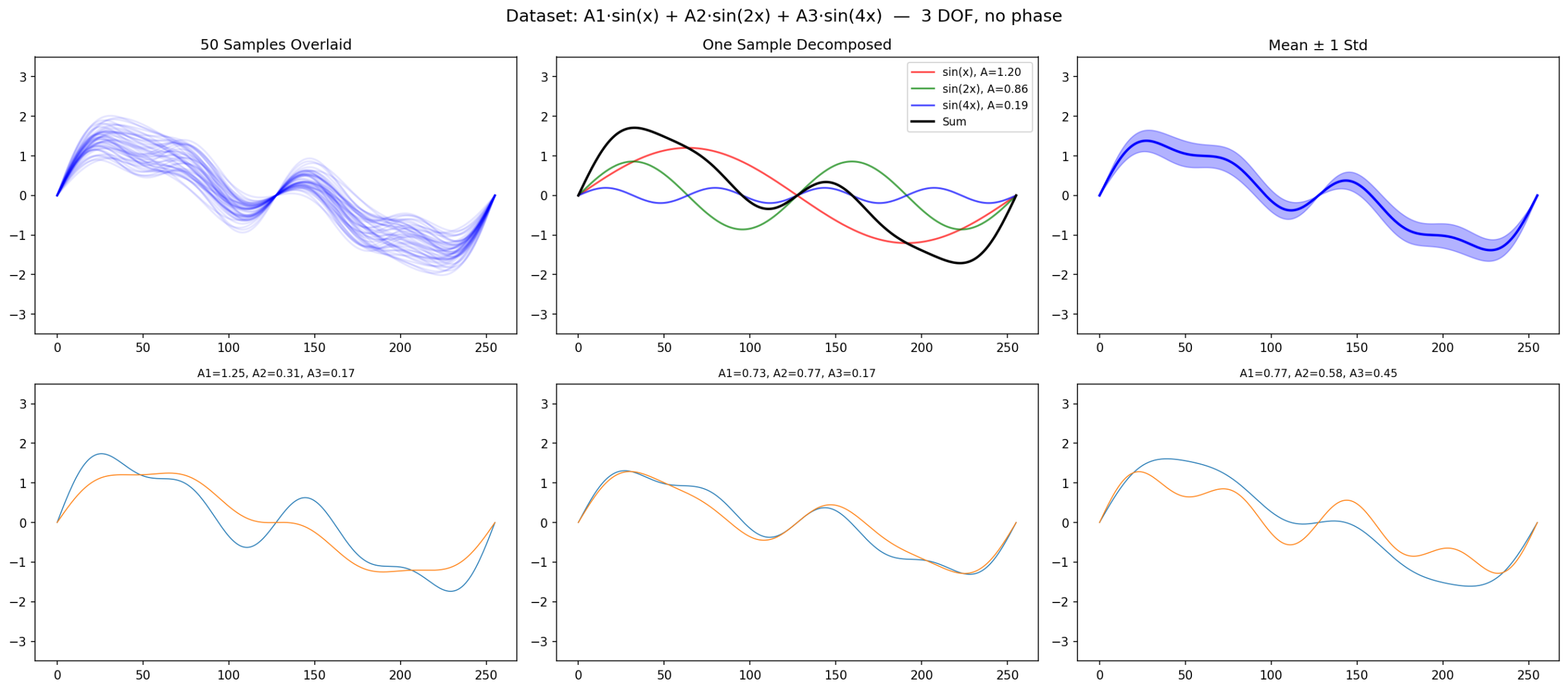
2. The Dataset
2,000 sine waves, each with small random variations in amplitude, frequency, and phase:
def generate_sine_dataset(n_samples, n_points):
    x = np.linspace(0, 2 * np.pi, n_points)
    data = []
    for _ in range(n_samples):
        amp = np.random.uniform(0.8, 1.2)
        phase = np.random.uniform(-0.3, 0.3)
        freq = np.random.uniform(0.9, 1.1)
        y = amp * np.sin(freq * x + phase)
        data.append(y)
    return torch.tensor(np.array(data), dtype=torch.float32)
Three degrees of freedom (amplitude, frequency, phase) in a 256-dimensional space. This ratio will become important later.
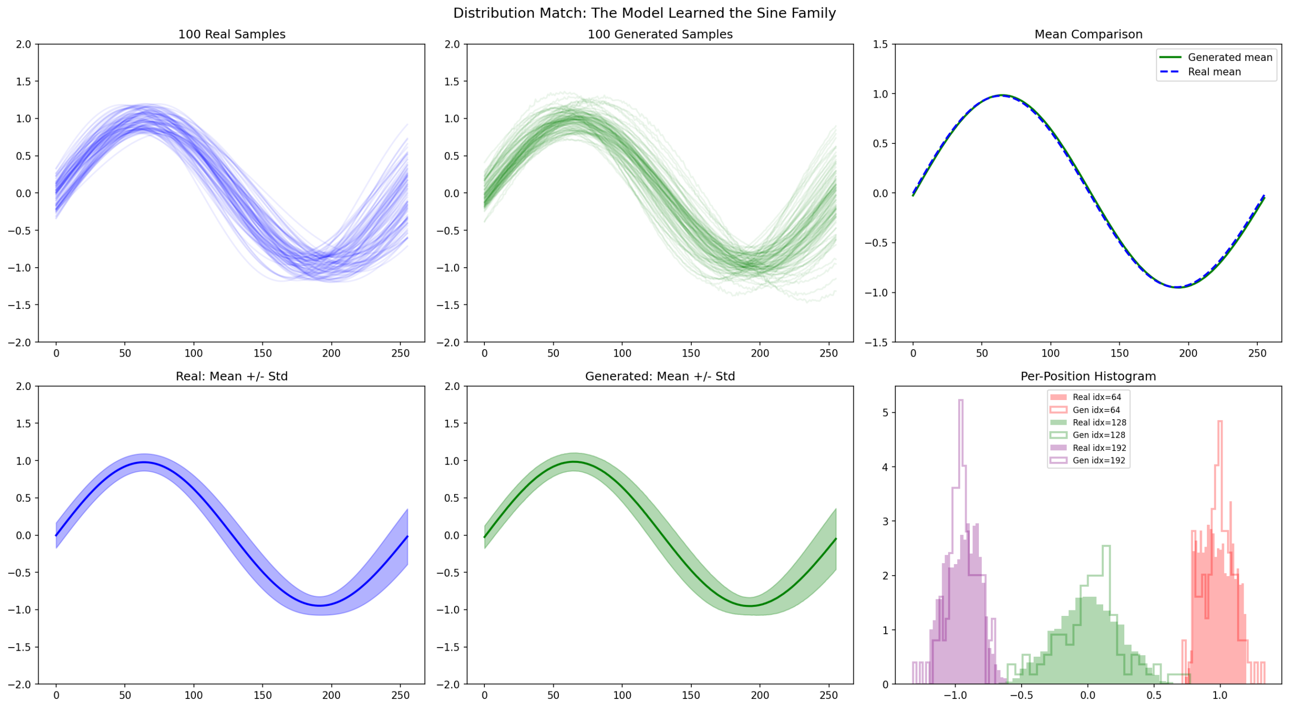
Left: 100 samples overlaid. Middle: mean ± 1 std. Right: per-position histograms.
3. Forward Process
The DDPM forward process (Ho et al., 2020) adds noise via the closed-form formula:
$$ x_t = \sqrt{\bar{\alpha}_t} \cdot x_0 + \sqrt{1 – \bar{\alpha}_t} \cdot \varepsilon $$
Where does this formula come from? It is not an assumption — it is the closed-form solution of a simple recurrence. Starting from:
$$ x_t = \sqrt{\alpha_t} \cdot x_{t-1} + \sqrt{1 – \alpha_t} \cdot z_t $$
and recursively expanding \(x_1, x_2, x_3, \ldots \), the signal component becomes a product of \(\sqrt{\alpha} \) terms, while the noise becomes a weighted sum of independent Gaussians. Because a weighted sum of Gaussians is still Gaussian, the entire process collapses into a single noise term:
$$ x_t = \sqrt{\bar{\alpha}_t} \cdot x_0 + \sqrt{1 – \bar{\alpha}_t} \cdot \varepsilon $$
This is why we can sample any timestep directly without simulating all intermediate steps.
Standard linear beta schedule:
betas = torch.linspace(1e-4, 0.02, 1000)
alphas = 1 - betas
alpha_bar = torch.cumprod(alphas, dim=0)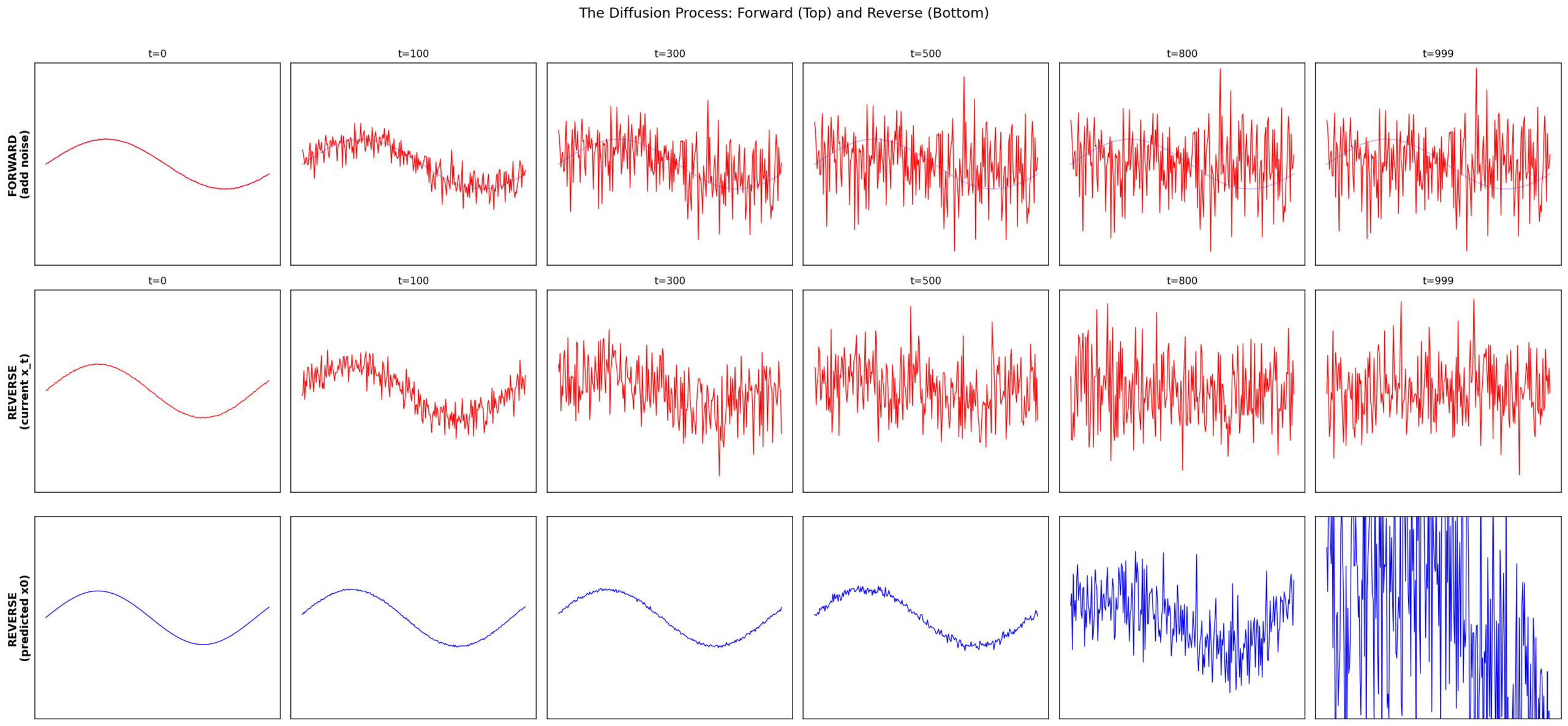
A sine wave dissolving into noise. Signal-noise crossover occurs around t=250.
Why not add all noise at once? Because the reverse problem would become impossible. If a single step destroyed most of the signal, the model would need to reconstruct structure from near-pure noise in one shot. Instead, diffusion turns a hard problem into 1,000 easy ones: each step removes a tiny amount of noise from an almost-clean signal.
An intuitive analogy: the forward process is like dust gradually accumulating on a camera lens. At early timesteps (left), the scene is almost fully visible. At middle timesteps (center), structure is still recognizable. At late timesteps (right), the original scene is nearly lost. The model learns to clean the lens one step at a time — each step only needs to remove a thin layer of dust.
In other words, diffusion works by transforming a global, difficult inverse problem into a sequence of local, tractable ones.
4. Model and Training
MLP with sinusoidal time embeddings and residual connections (5.3M parameters). Deliberately not a UNet — we want to see what the math provides, not the architecture.
class SinusoidalTimeEmbedding(nn.Module):
    def __init__(self, dim):
        super().__init__()
        self.dim = dim

    def forward(self, t):
        half = self.dim // 2
        freqs = torch.exp(
            -np.log(10000) * torch.arange(half, device=t.device).float() / half
        )
        args = t.float().unsqueeze(1) * freqs.unsqueeze(0)
        return torch.cat([args.sin(), args.cos()], dim=-1)


class ResidualBlock(nn.Module):
    def __init__(self, dim, time_dim):
        super().__init__()
        self.net = nn.Sequential(
            nn.Linear(dim, dim), nn.GELU(), nn.Linear(dim, dim),
        )
        self.time_mlp = nn.Linear(time_dim, dim)
        self.norm = nn.LayerNorm(dim)

    def forward(self, x, t_emb):
        h = self.norm(x)
        h = self.net(h) + self.time_mlp(t_emb)
        return x + h


class DiffusionMLP(nn.Module):
    def __init__(self, signal_dim=256, hidden_dim=512, time_dim=128, n_blocks=6):
        super().__init__()
        self.time_embed = nn.Sequential(
            SinusoidalTimeEmbedding(time_dim),
            nn.Linear(time_dim, hidden_dim), nn.GELU(),
            nn.Linear(hidden_dim, hidden_dim),
        )
        self.input_proj = nn.Linear(signal_dim, hidden_dim)
        self.blocks = nn.ModuleList([
            ResidualBlock(hidden_dim, hidden_dim) for _ in range(n_blocks)
        ])
        self.output_proj = nn.Sequential(
            nn.LayerNorm(hidden_dim), nn.Linear(hidden_dim, signal_dim),
        )

    def forward(self, x_t, t):
        t_emb = self.time_embed(t)
        h = self.input_proj(x_t)
        for block in self.blocks:
            h = block(h, t_emb)
        return self.output_proj(h)
Training: standard DDPM objective — sample random timestep, add noise, predict the noise, minimize MSE.
for epoch in range(500):
    for batch in dataloader:
        x0 = batch.to(device)
        t = torch.randint(0, num_timesteps, (x0.shape[0],), device=device)

        noise = torch.randn_like(x0)
        x_t = sqrt_alpha_bar[t].unsqueeze(1) * x0 \
            + sqrt_one_minus_alpha_bar[t].unsqueeze(1) * noise

        noise_pred = model(x_t, t)
        loss = F.mse_loss(noise_pred, noise)

        optimizer.zero_grad()
        loss.backward()
        torch.nn.utils.clip_grad_norm_(model.parameters(), 1.0)
        optimizer.step()
Final loss after 500 epochs: ~0.005.
An important subtlety: training samples timesteps randomly — the model never sees the sequence t=999, 998, 997, … during training. It learns to denoise at each noise level independently. Only during inference are the steps chained together sequentially. This means the model learns a family of denoising functions indexed by timestep, not a single sequential process.
5. Generating from Noise
Reverse sampling follows Algorithm 2 from Ho et al.:
@torch.inference_mode()
def ddpm_sample(model, n_samples=8):
    x = torch.randn(n_samples, n_points, device=device)

    for t_val in reversed(range(num_timesteps)):
        t_batch = torch.full((n_samples,), t_val, device=device, dtype=torch.long)
        eps_pred = model(x, t_batch)

        beta_t = betas[t_val]
        coef = beta_t / sqrt_one_minus_alpha_bar[t_val]
        mu = (1 / alphas[t_val].sqrt()) * (x - coef * eps_pred)

        if t_val > 0:
            sigma = posterior_variance[t_val].sqrt()
            x = mu + sigma * torch.randn_like(x)
        else:
            x = mu
    return x.cpu()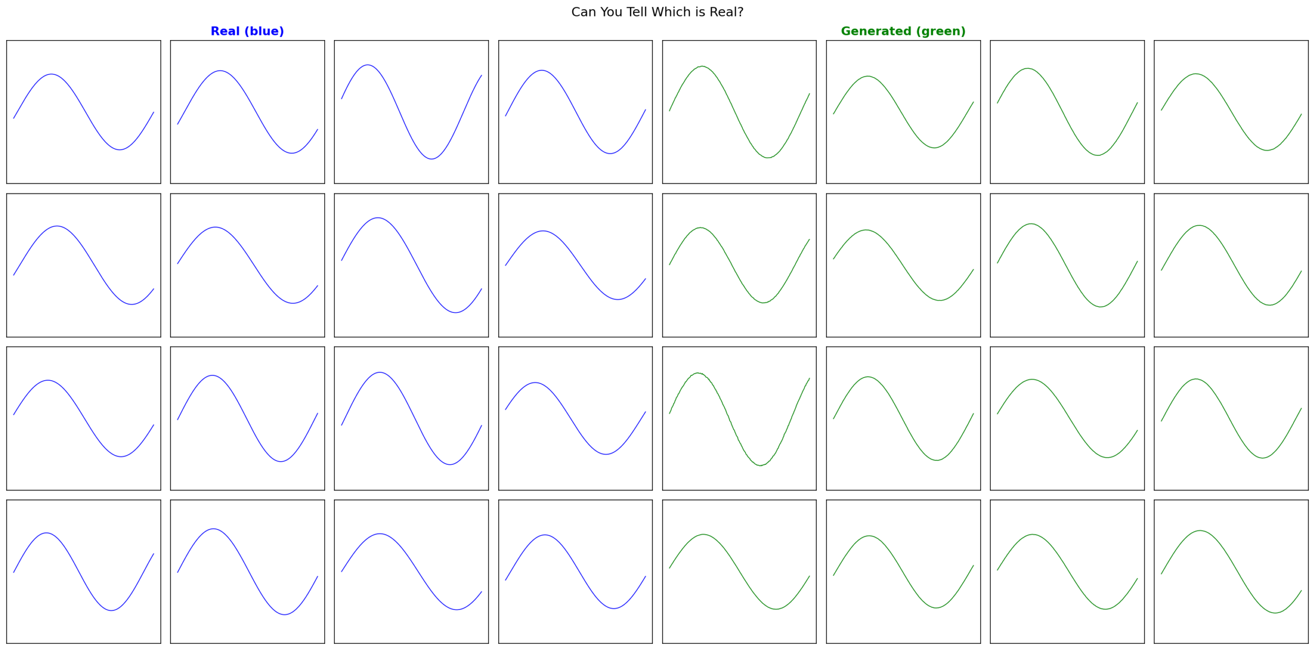
Real (blue) vs generated (green). Statistically indistinguishable.
6. What Does the Model Learn?
6.1 Noise Prediction at Different Timesteps
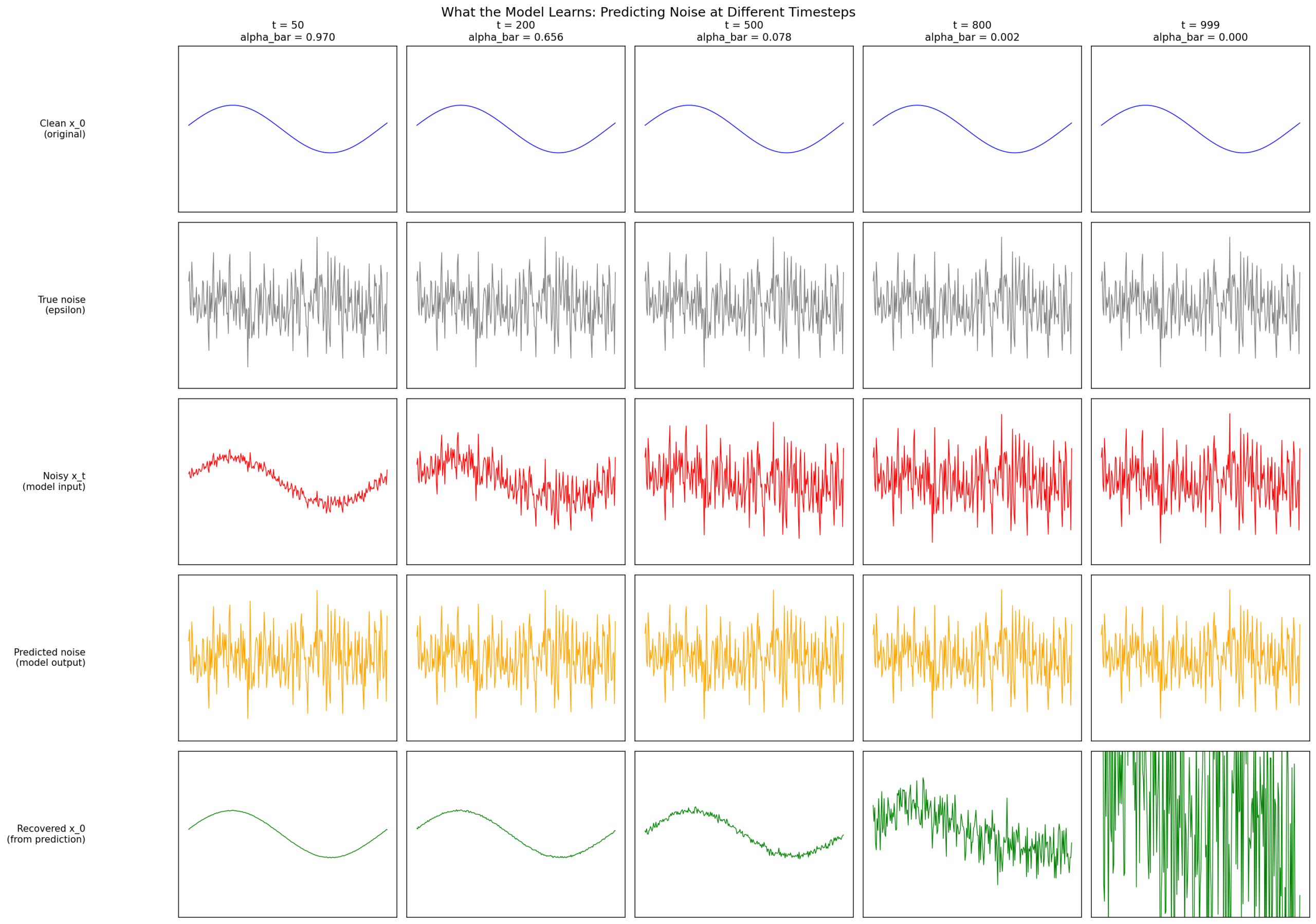
Five timesteps, five rows: clean \(x_0 \), true noise, noisy \(x_t \), predicted noise, recovered \(x_0 \). At t=50 the model makes precise estimates. At t=999 recovery is a rough guess. Key tradeoff: noise MSE improves at high t, but recovery MSE explodes due to \(1/\sqrt{\bar{\alpha}} \) amplification.
Are the noise predictions just random Gaussian samples? No. Even though the added noise is Gaussian, the model’s predictions are conditioned on \(x_t \) — which still contains structure from the original signal. If you average many predicted noise samples at the same timestep, you recover structure (e.g., a sine shape), precisely because the predictions are signal-dependent. The model does not memorize random noise — it learns a mapping from noisy input to noise estimate, conditioned on both \(x_t \) and \(t \).
6.2 Anatomy of a Reverse Step
What exactly happens in one step? At t=500 the model receives noisy input, predicts noise, estimates \(x_0 \), computes the posterior mean, and adds fresh noise to produce \(x_{499} \). Net effect: ~0.08 dB SNR improvement.
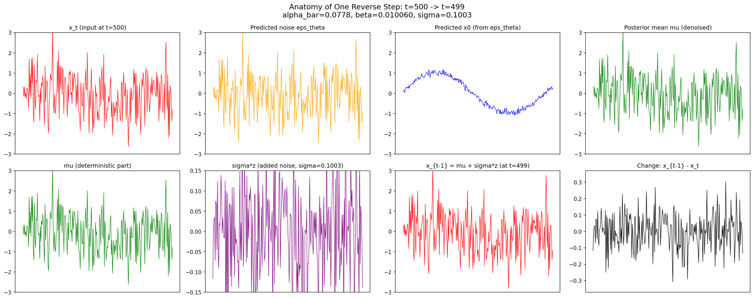
Single step decomposed: \(x_t \rightarrow \) predicted \(\varepsilon \rightarrow x_0 \) estimate \(\rightarrow \) posterior mean \(\rightarrow \) noise injection \(\rightarrow x_{t-1} \).
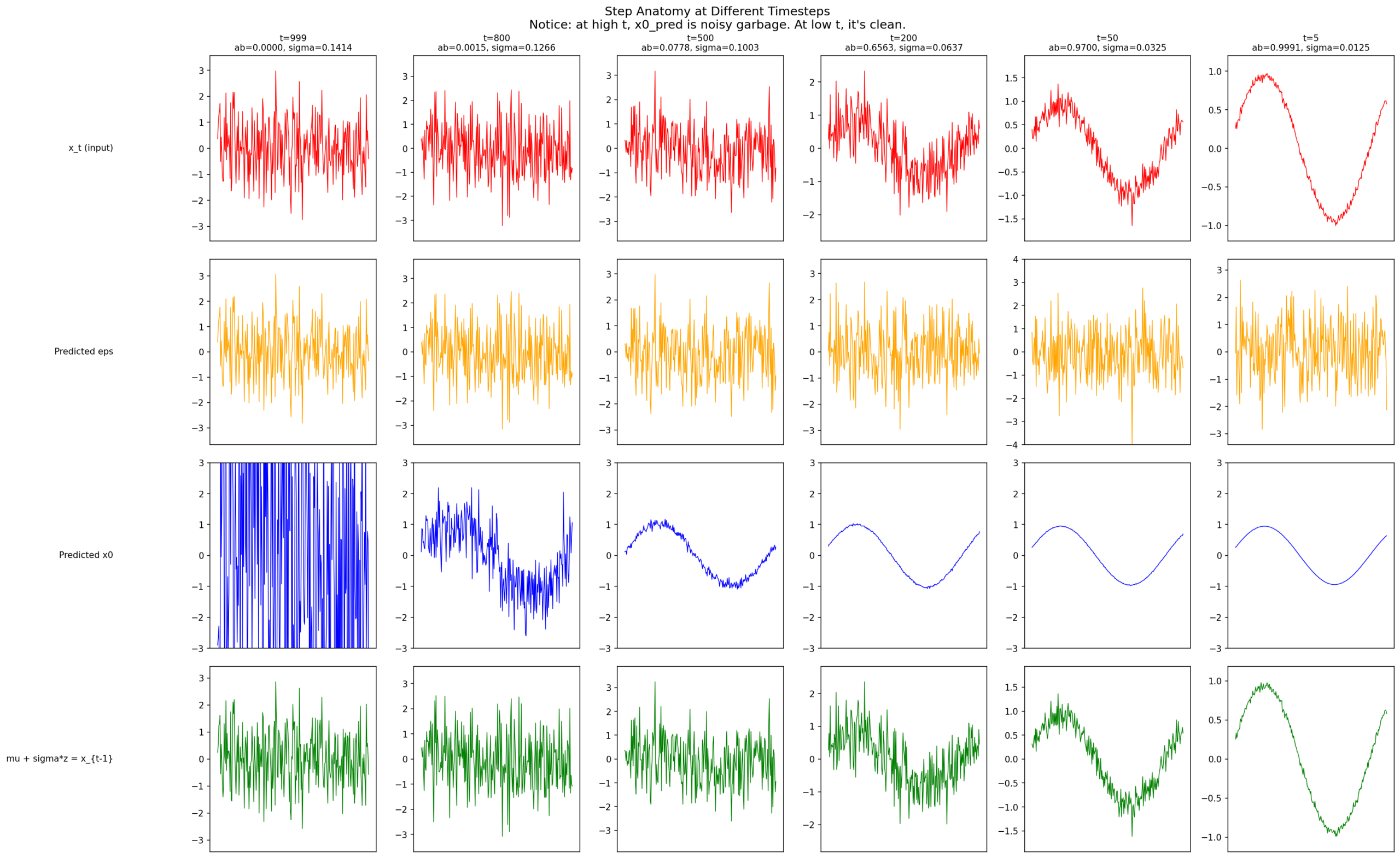
Same anatomy at t = 999, 800, 500, 200, 50, 5. Early steps: coarse structure. Late steps: fine corrections.
6.3 Why It Works
The model learns one function: \(\varepsilon_\theta(x_t, t) \rightarrow \) predicted noise. At each step, \(\beta_t \approx 0.008 \), meaning 99.2% of the signal survives from one step to the next. So the task at each step is: “given something that is 99.2% signal, estimate the 0.8% noise.” Easy. Chain 1,000 such easy tasks, and you accomplish what seems impossible: creating a clean signal from pure noise.
6.4 What the Model Is Really Learning
The model is trained to predict noise, but this has a deeper interpretation. At each timestep, it learns how the data distribution behaves locally — effectively estimating the direction toward higher probability regions.
In more advanced terms, diffusion models learn the gradient of the log-density of the data distribution. This is why the reverse process works: each step moves the sample slightly toward the data manifold, guided by this learned structure.
You do not need this interpretation to implement diffusion — but it explains why the method works so reliably across domains.
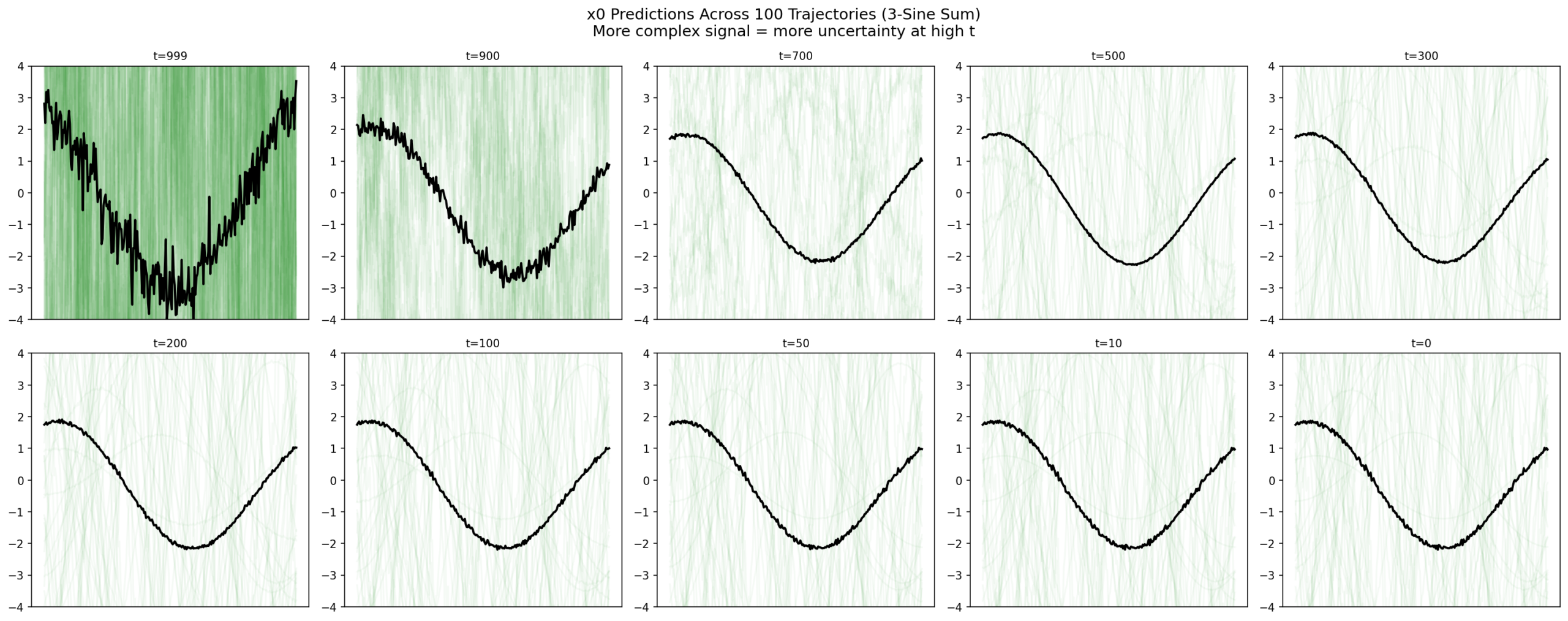
7. 100 Parallel Trajectories
We run 100 independent reverse processes from different noise seeds and track every trajectory.
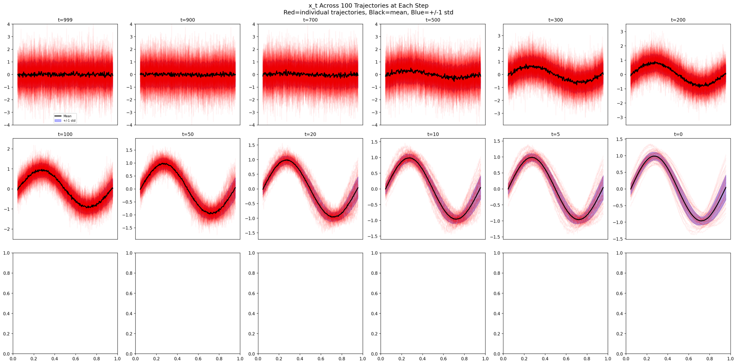
\(x_t \) evolution: scattered noise at t=999 → sine structure by t=500 → diverse clean signals at t=0.
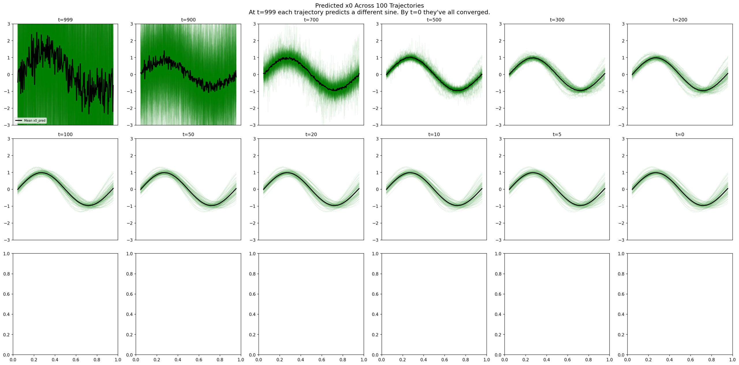
\(x_0 \) predictions: chaos at t=999, commitment by t=300, locked in at t=0. The final spread is the learned distribution’s diversity, not uncertainty.
7.1 The Commitment Table
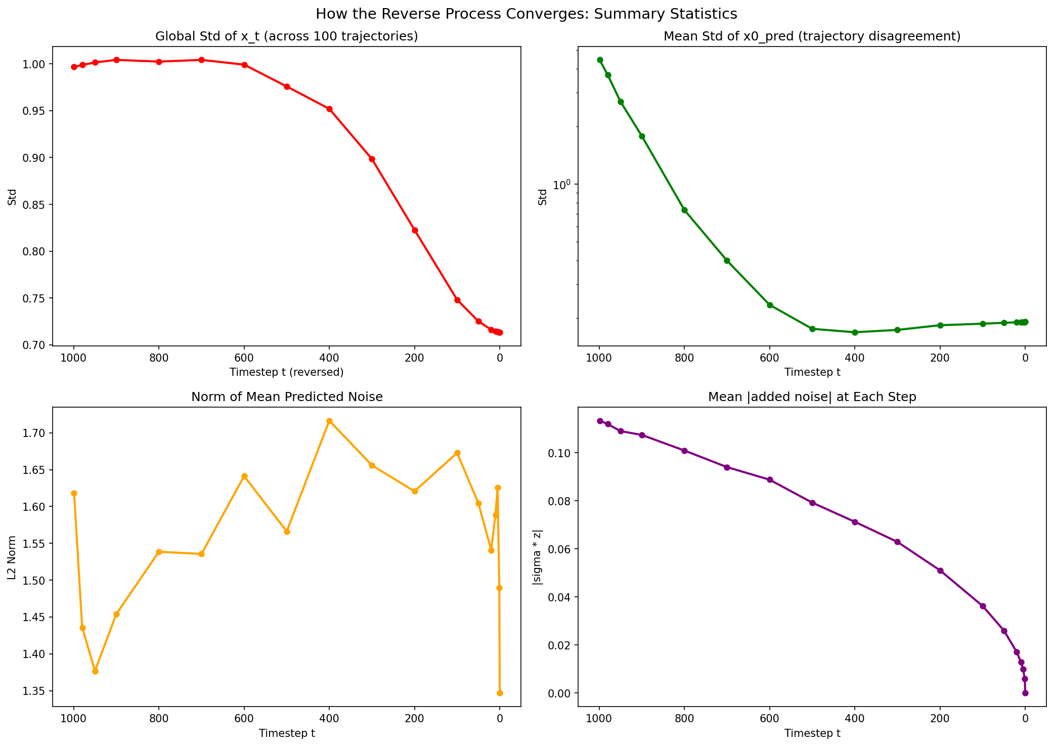
t=999: x0_pred std = 4.45   (chaos)
t=800: x0_pred std = 0.73   (narrowing)
t=500: x0_pred std = 0.18   (committed)
t=0:   x0_pred std = 0.19   (locked in = dataset diversity)
The drop from 0.73 to 0.18 between t=800 and t=500 is where the model “recognizes” which sine each trajectory is heading toward.
7.2 The Denoising Budget
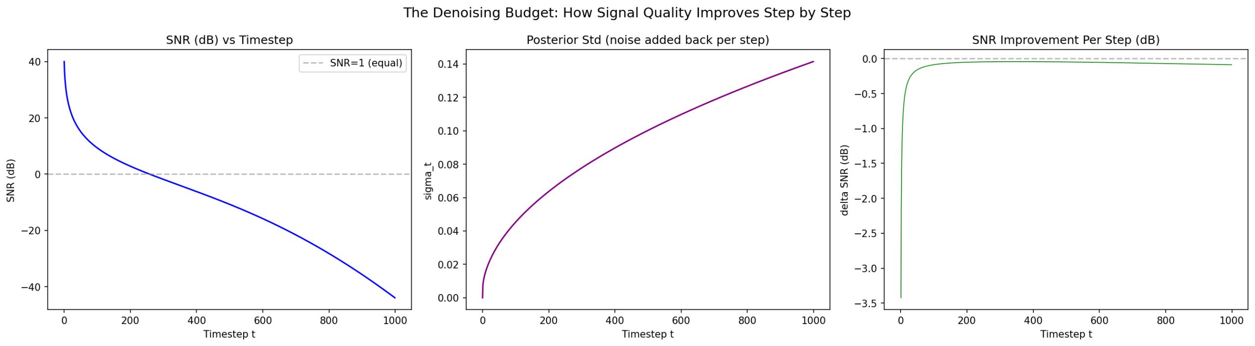
~0.08 dB per step × 1,000 steps ≈ 80 dB total denoising.
8. When Does Diffusion Fail?
The single sine has 3 DOF in 256 dimensions. What happens if we increase the degrees of freedom?
8.1 Three Sines, Random Phases (6 DOF)
def generate_3sine_dataset(n_samples, n_points):
    x = np.linspace(0, 2 * np.pi, n_points)
    data = []
    for _ in range(n_samples):
        A1 = np.random.uniform(0.5, 1.5)
        A2 = np.random.uniform(0.3, 1.0)
        A3 = np.random.uniform(0.1, 0.5)
        phi1 = np.random.uniform(-np.pi, np.pi)
        phi2 = np.random.uniform(-np.pi, np.pi)
        phi3 = np.random.uniform(-np.pi, np.pi)
        y = A1*np.sin(x + phi1) + A2*np.sin(x/2 + phi2) + A3*np.sin(x/16 + phi3)
        data.append(y)
    return torch.tensor(np.array(data), dtype=torch.float32)
6 DOF: 3 amplitudes + 3 phases over [-π, π]. Same model, same training. Loss: 0.01 (2× worse).

8.2 Result: Mode Collapse
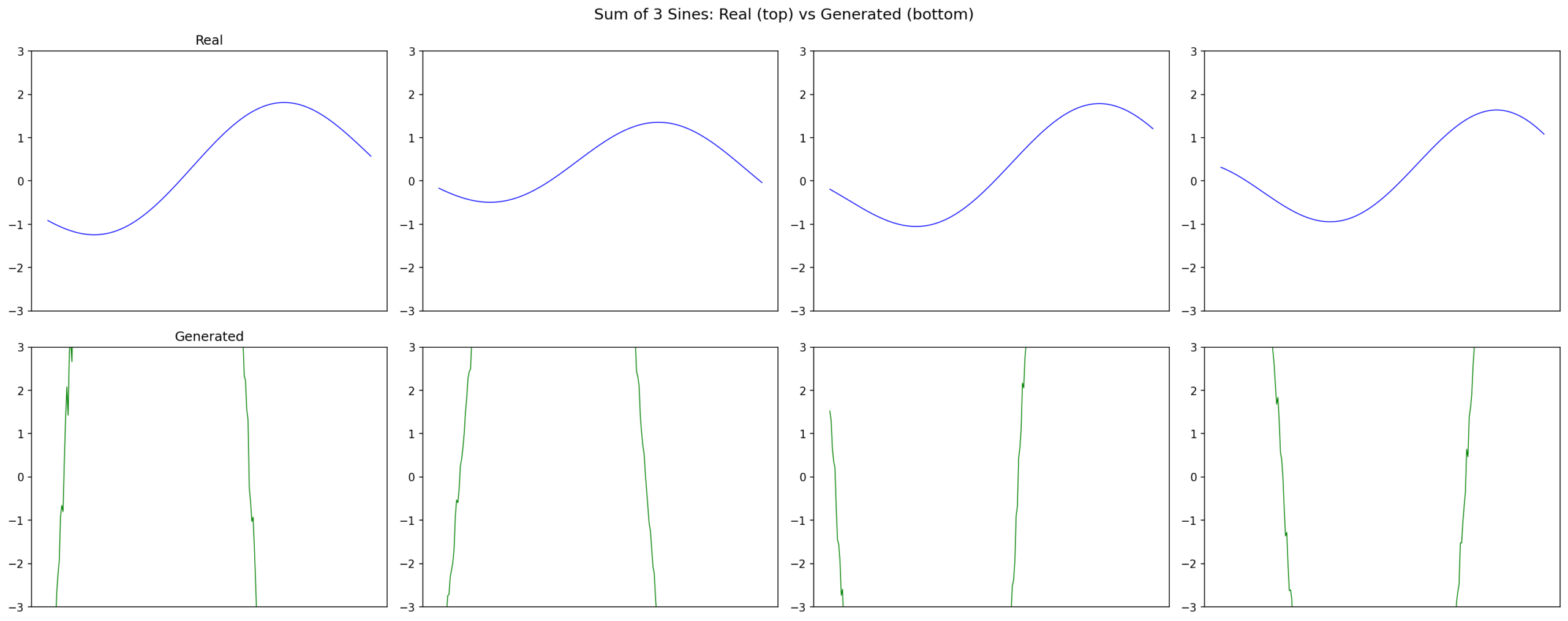
Real (top) vs generated (bottom). All generated samples collapse to one rigid template.
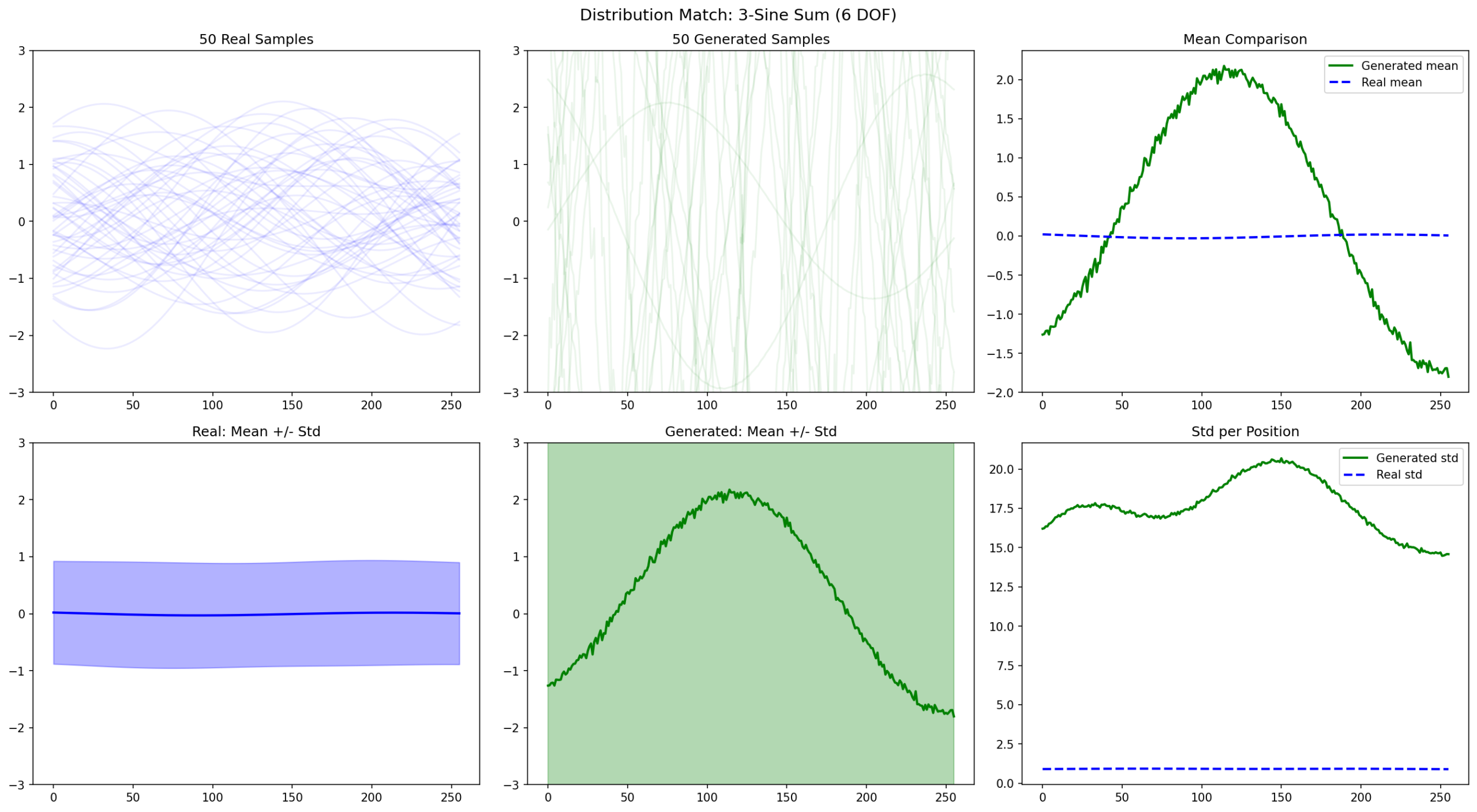
Real mean ≈ 0 (phases cancel). Generated mean: a large fixed waveform. Generated std is 15-20× the real std.
All 100 trajectories collapse to the same template instead of producing diverse outputs.
8.3 The Hypothesis
Hypothesis A: Signal complexity — three frequencies are harder than one.
Hypothesis B: The phases. Original experiment: phase ±0.3 rad. This experiment: phase ±π. Full-circle phase variation scatters signals across the entire 256D space.
Analogy: Stable Diffusion generates butterflies that are always centered, facing forward. Variation is in texture and color — not in whether the butterfly is rotated 180°. The data manifold is compact. Random phases destroy that compactness.
Another way to interpret this: the forward process is fixed and well-behaved, but the reverse process must learn how to navigate the data distribution. If the manifold is too spread out, there is no consistent “direction” for the model to follow — and the reverse process collapses.
9. Isolating the Variable
Same three sines, but fix phases to zero. Only amplitudes vary:
def generate_3sine_v2(n_samples, n_points):
    x = np.linspace(0, 2 * np.pi, n_points)
    data = []
    for _ in range(n_samples):
        A1 = np.random.uniform(0.5, 1.5)
        A2 = np.random.uniform(0.3, 1.0)
        A3 = np.random.uniform(0.1, 0.5)
        y = A1*np.sin(x) + A2*np.sin(2*x) + A3*np.sin(4*x)
        data.append(y)
    return torch.tensor(np.array(data), dtype=torch.float32)
Still 3 DOF. Richer waveform than single sine. Only change: no random phases.
9.1 Result: Perfect
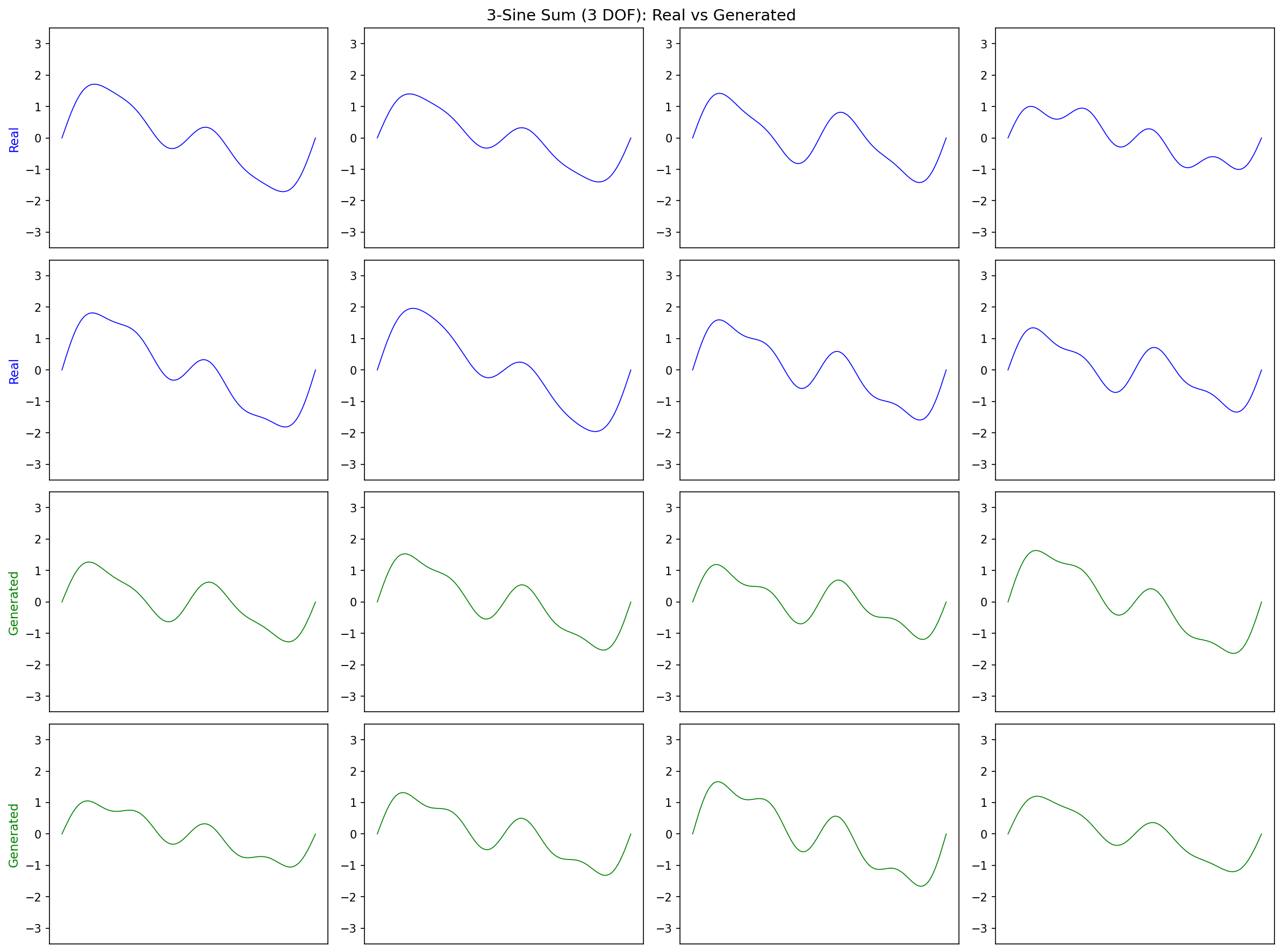
Generated samples (green) are indistinguishable from real (blue).
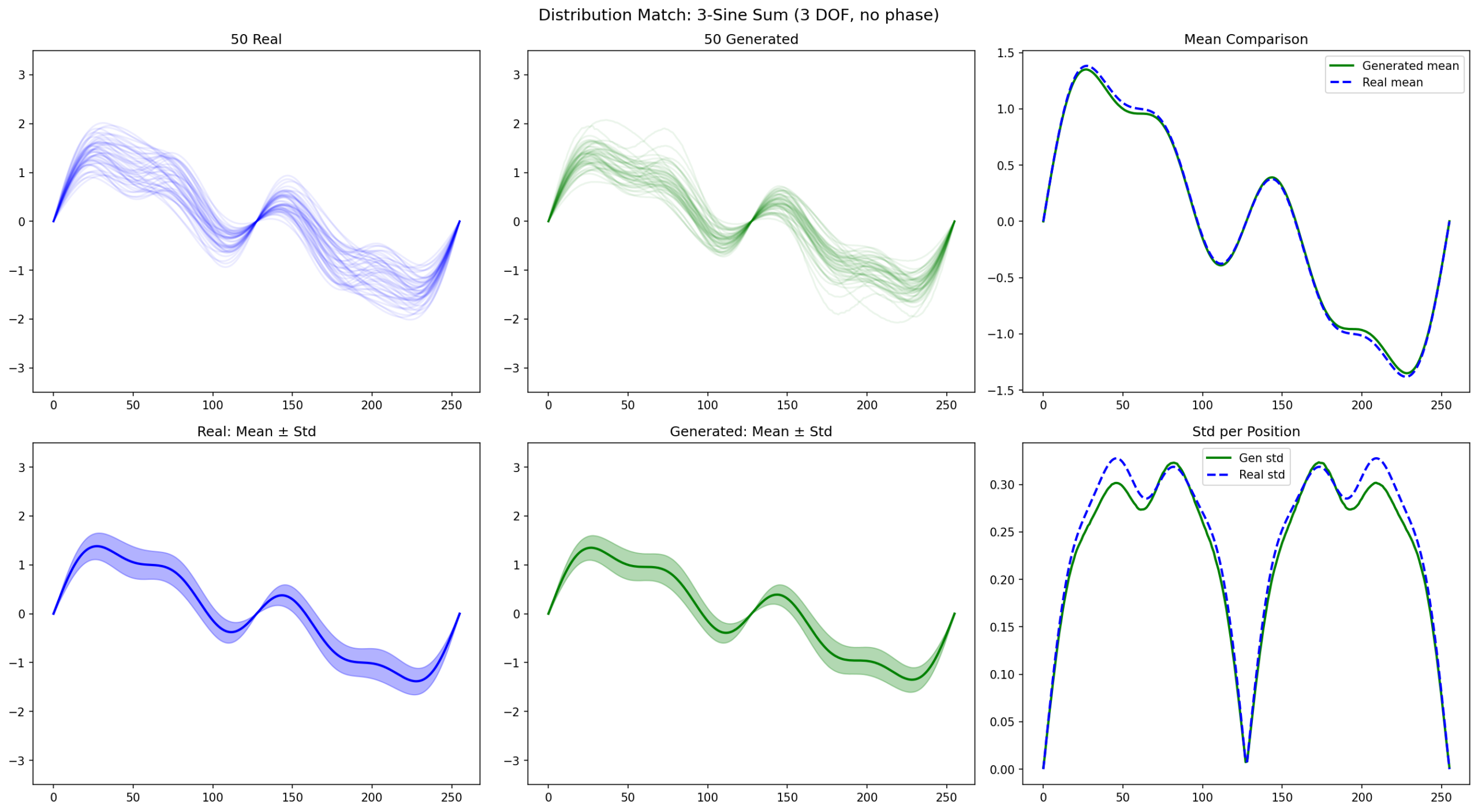
Mean and std overlap almost perfectly between real and generated.
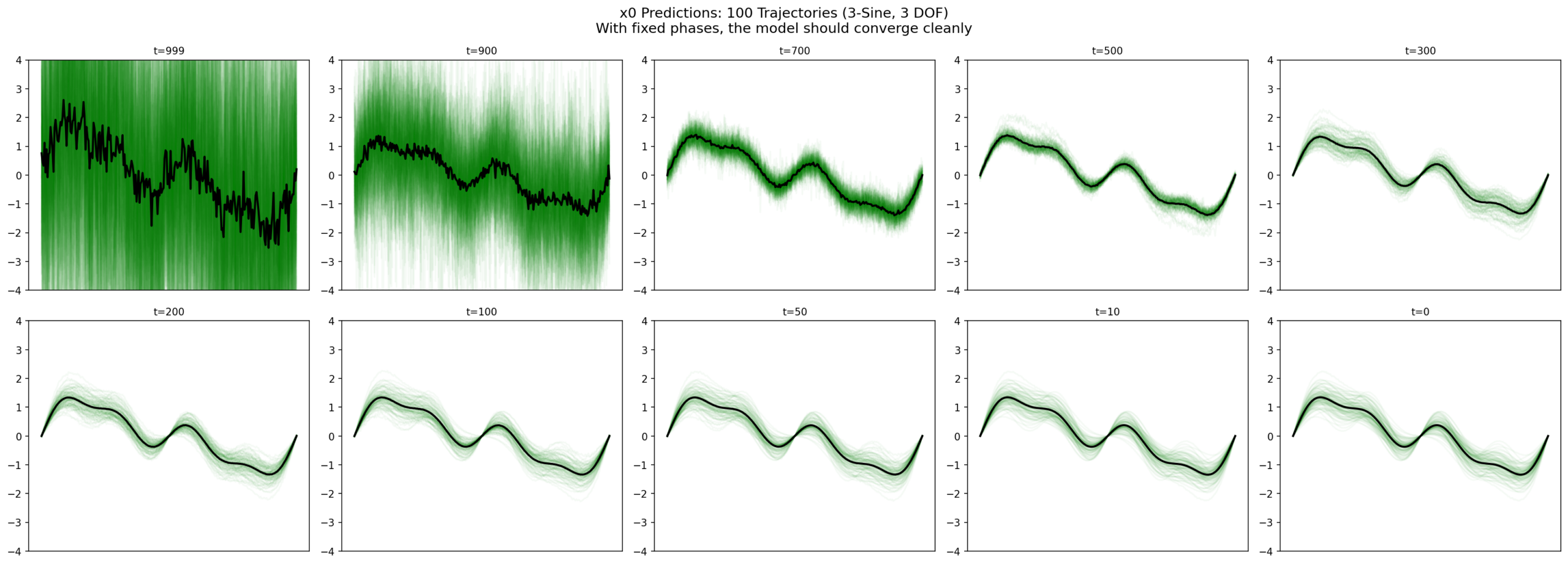
Same clean convergence pattern as the single-sine experiment.
9.2 Conclusion
Same model. Same 3 DOF. Same training. The only difference: phase = 0 vs phase ∈ [-π, π]. One succeeds. The other collapses. It is not signal complexity — it is manifold compactness.
From a broader perspective, diffusion models do not “solve an equation” in the classical sense. The forward process is known and fixed, but the reverse process depends on the unknown data distribution. The neural network learns this reverse dynamic from data, effectively reconstructing the structure of the distribution through local denoising steps.
10. Implications for Image Diffusion
| 1D Sine | Image Domain |
|---|---|
| 256 values | 64×64×3 = 12,288 pixels |
| MLP | UNet |
| Small phase (±0.3 rad) | Centered, aligned data |
| Full phase (±π) | Arbitrary rotations |
| 3 DOF / 256 dims | ~100-1000 DOF / 12,288 dims |
Diffusion models succeed when data lives on a compact, low-dimensional manifold. This is why centered faces work, why conditioning helps (narrows the manifold), and why aggressive spatial augmentation can hurt.
Code
Three Colab-ready scripts (no argparse, just run):
- diffusion_1d_sine_v3.py — Single-sine DDPM with all diagnostics
- diffusion_3sines.py — 6-DOF failure (random phases)
- diffusion_3sines_v2.py — 3-DOF success (fixed phases)
That covers our exploration of diffusion through 1D signals. The key insight: understanding when and why a model fails teaches more than any number of successful runs. Take care! 🙂