#008 Shallow Neural Network
Vectorizing Across Multiple Training Examples
In this post we will see how to vectorize across multiple training examples. The outcome will be similar to what we saw in Logistic Regression. Equations we defined in previous post are these:
\(z^{[1]} =\textbf{W}^{[1]} x + b ^{[1]} \)
\(a^{[1]} = \sigma ( z^{[1]} ) \)
\(z^{[2]} = \textbf{W}^{[2]} a^{[1]} + b ^{[2]} \)
\(a^{[2]} = \sigma ( z^{[2]} ) \)
These equations tell us how, when given an input feature vector \(x \), we can generate predictions.
\(x \rightarrow a^{[2]} = \hat{y} \)
If we have \(m \) training examples we need to repeat this proces \(m \) times. For each training example, or for each feature vector that looks like this:
\(x^{(1)} \rightarrow a^{[2](1)} = \hat{y} \)
\(x^{(2)} \rightarrow a^{[2](2)} = \hat{y} \)
\(\vdots \)
\(x^{(m)} \rightarrow a^{[2](m)} = \hat{y} \)
The notation \( a^{[2](i)} \) means that we are talking about activation in the second layer that comes from \(i^{th} \) training example. In the square parentheses we write number of a layer, and number in the parentheses refers to the particular training example.
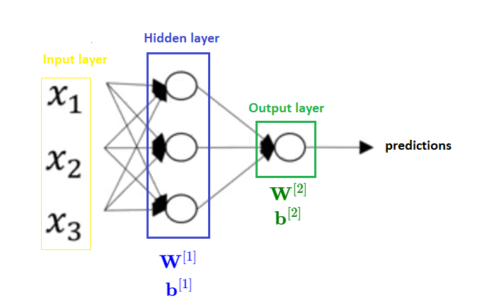
We will now see equations for one hidden layer neural network which is presented in the following picture.
To do calculations written above, we need a for loop that would look like this:
\(for\enspace i \enspace in \enspace range( m ):\)
\(\color {Blue} {z^{[1](i)}} = \textbf{W}^{[1]} x^{(i)} + b ^{[1]} \)
\(\color {Blue} {a^{[1](i)}} = \sigma ( \color {Blue} {z^{[1](i)}} ) \)
\(\color {Green} {z^{[2](i)} } = \textbf{W}^{[2]} \color {Blue} {a^{[1](i)}}+ b ^{[1]} \)
\(\color {Green} {a^{[2](i)} }= \sigma ( \color {Green} {z^{[2](i)}} ) \)
Now our task is to vectorize all these equations and get rid of this for loop.
We will recall definitions of some matrices. Martix \(\textbf{X} \) was defined as we have put all feature vectors in columns of a matrix, actually we stacked feature vectors horizontally. Every column in matrix \(\textbf{X} \) is a feature vector for one training example, so the dimension of this matrix is \((number\enspace of \enspace features \enspace in \enspace every\enspace vector, \enspace number \enspace of\enspace training\enspace examples)\). Matrix \(\textbf{X} \) is defined as follows:
$$ \textbf{X} = \begin{bmatrix} \vert & \vert & \dots & \vert \\ x^{(1)} & x^{(2)} & \dots & x^{(m)} \\ \vert & \vert & \dots & \vert \end{bmatrix} $$
In the same way we can get the \(\textbf{ Z}^{[1]} \) matrix, as we stack horizontally values \(z^{[1](1)} … z^{[1](m)} \) :
$$ \textbf{Z}^{[1]} = \begin{bmatrix} \vert & \vert & \dots & \vert \\ z^{[1](1)} & z^{[1](2)} & \dots & z^{[1](m)} \\ \vert & \vert & \dots & \vert \end{bmatrix} $$
Similiar is with values \(a^{[1](1)} … a^{[1](m)} \) which are the activations in the first node for paritcular training example:
\(\textbf{A}^{[1]}=\begin{bmatrix} \vert & \vert & \dots & \vert \\ a^{[1](1)} & a^{[1](2)} & \dots & a^{[1](m)} \\ \vert & \vert & \dots & \vert\end{bmatrix} \)
An element in the first row and in the first column of a matrix \( \textbf{A}^{[1]} \) is an activation of the first hidden unit and the first training example. In the first row of this matrix there are activations in the first hidden unit among all training examples. The same is with another rows in this matrix. Next element, element in the first row and the second column, is an activation of the first unit from second training element and so on.
$$ A^{[1]} = \begin{bmatrix} 1^{st} unit \enspace of \enspace 1.tr. example & 1^{st} unit \enspace of \enspace 2^{nd}tr. example & \dots & 1^{st} unit \enspace of \enspace m^{th}.tr. example \\ 2^{nd}unit \enspace of \enspace 1^{st}tr. example & 2^{nd} unit \enspace of \enspace 2^{nd}tr. example & \dots & 2^{nd} unit \enspace of \enspace m^{th}tr. example \\ the \enspace last \enspace unit \enspace of \enspace 1^{st}tr. example & the \enspace last \enspace unit \enspace of \enspace2^{nd}tr. example & \dots & the \enspace last \enspace unit \enspace of m^{th}tr. example \end{bmatrix} $$
To conclude, in matrix \(\textbf{A}^{[1]} \) there are activation of the first hidden layer of a Neural Network. In every column there are activations for each training example, so number of columns in this matrix is equal to the number of training examples. In the first row of this matrix there are activations first hidden unit among all training examples.
Vectorized version of previous calculations looks like this:
\(\color {Blue} {\textbf{ Z}^{[1]}} = \textbf{W}^{[1]} \textbf{X} + b^{[1]} \)
\(\color {Blue} {\textbf{ A}^{[1]}} = \sigma(\color {Blue} {\textbf{ Z}^{[1]}}) \)
\(\color {Green} {\textbf{ Z}^{[2]}} = W^{[2]} \color {Blue} {\textbf{ A}^{[1]}} + b^{[2]} \)
\(\color {Green} {\textbf{ A}^{[2]} }= \sigma(\color {Green} {\textbf{ Z}^{[2]}}) \)
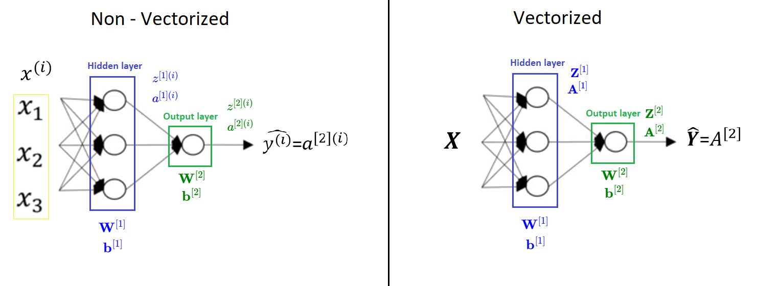
In the following picture we can see comparation of vectorized and non-vectorized version.
Explanation for Vectorized Implementation
Let’s go through part of a forward propagation calculation for a few examples. \(\color{Orange} {x^{(1)}} \) , \(\color{Green}{x^{(2)} } \) and \(\color{Blue} {x^{(3)} }\) are 3 input vectors, those are three examples of feature vectors or three training examples.
\(z^{[1](1)} = \textbf{W}^{[1]} \color{Orange} {x^{(1)}} + b^{[1]} \)
\(z^{[1](2)} =\textbf{W}^{[1]} \color{Green} {x^{(2)}} + b^{[1]} \)
\(z^{[1](3)} = \textbf{W}^{[1]} \color{Blue} {x^{(2)}} + b^{[1]} \)
We will ignore \( b^{[1]} \) values, to simplify these calculations, so we have following equations:
\(z^{[1](1)} = \textbf{W}^{[1]} \color{Orange} {x^{(1)}} \tag {1}\)
\(z^{[1](2)} = \textbf{W}^{[1]} \color{Green} {x^{(2)}} \tag {2} \)
\(z^{[1](3)} = \textbf{W}^{[1]} \color{Blue} {x^{(2)}} \tag {3} \)
Our training set \(\textbf{X} \) we will get as we stack our three training examples horizontally.
$$ \textbf{X} = \begin{bmatrix} \color{Orange} \vert & \color{Green}\vert & \color{Blue} \vert \\ \color{Orange} {x^{(1)}} & \color{Green} {x^{(2)}}& \color{Blue} {x^ {(2)}}\\ \color{Orange}\vert & \color{Green} \vert & \color{Blue} \vert \end{bmatrix} $$
So when we multiply matrix \( \textbf{W}^{[1]} \) with each training example we get following calculation:
\(\textbf{W}^{[1]} \color{Orange} {x^{(1)} }= \begin{bmatrix} \color{Orange}{\cdot} \\ \color{Orange}{\cdot} \\ \color{Orange}{\vdots} \\ \color{Orange}{\cdot} \end{bmatrix} \) \(\textbf{ W}^{[1]} \color{Green} {x^{(2)} }= \begin{bmatrix} \color{Green}{\cdot} \\ \color{Green}{\cdot} \\ \color{Green}{\vdots} \\ \color{Green}{\cdot} \end{bmatrix} \) \(\textbf{W}^{[1]} \color{Blue} {x^{(3)} }= \begin{bmatrix} \color{Blue}{\cdot} \\ \color{Blue}{\cdot} \\ \color{Blue}{\vdots} \\ \color{Blue}{\cdot} \end{bmatrix} \)
And if we multiply \(\textbf{W}^{[1]} \) with matrix \( \textbf{X}\) we will get:
$$ \textbf{W}^{[1]} \textbf{X} =\begin{bmatrix} \textbf{W}^{[1]}\color{Orange} {x^{(1)} } & \textbf{W}^{[1]}\color{Green} {x^{(2)} } & \textbf{W}^{[1]}\color{Blue} {x^{(3)} } \end{bmatrix} = \begin{bmatrix} \color{Orange}{\cdot} & \color{Green}{\cdot} & \color{Blue}{\cdot} \\ \color{Orange}\vdots & \color{Green}\vdots & \color{Blue}\vdots \\ \color{Orange}{\cdot} & \color{Green}{\cdot} & \color{Blue}{\cdot} \end{bmatrix} = \begin{bmatrix} \color{Orange}{z^{[1](1)}} & \color{Green}{z^{[1](2)}} & \color{Blue}{z^{[1](3)}} \end{bmatrix} = \textbf{ Z}^{[1]} $$
If we now put back the value of \(b^{[1]} \) in equations \((1), (2) , (3) \) values are still correct. What actully happens when we add \(b^{[1]} \) values is that we end up with Python broadcasting.
With these equations we have justified that \(\textbf{ Z}^{[1]} = \textbf{W}^{[1]} \textbf{X} + b^{[1]} \) is a correct vectorization.
In the next post we will talk about acticvation functions and their derivatives.