#007 Neural Networks Representation

A quick overview
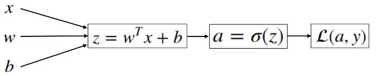
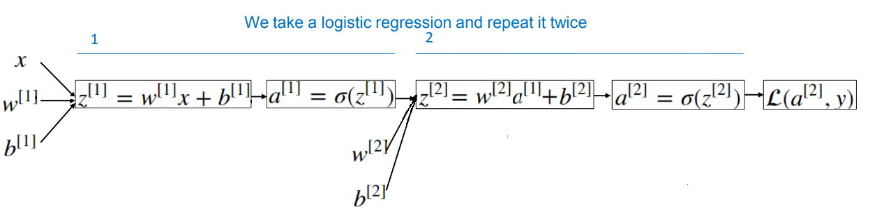
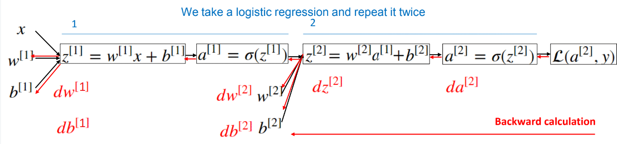
In previous posts we had talked about Logistic Regression and we saw how this model
corresponds to the following computation graph:
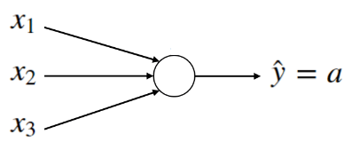
We have a feature vector \(x \)
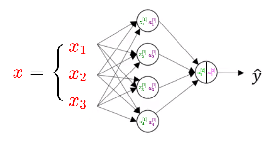
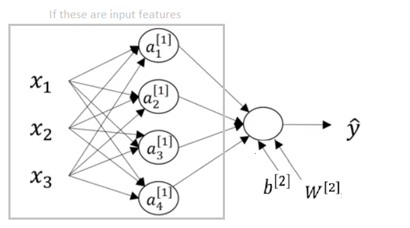
An example of a neural network is shown in the picture below. We can see we can form a neural network is created by stacking together several node units. One stack of nodes we will call a layer.
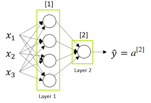
The first stack of nodes we will call Layer 1, and the second we will call Layer 2. We have two types of calculations in every node in the Layer 1, as well as in the Layer 2 ( which consists of just one node). We will use a superscript square bracket with a number of particular layer to refer to an activation function or a node that belongs to that layer. So, a superscript \([1] \) refers to the quantities associated with the first stack of nodes, called Layer 1. The same is with a superscript \([2] \) which refers to the second layer. Remember also that \(x^{(i)} \) refers to an individual training example.
The computation graph that corresponds to this Neural Network looks like this:

We have the following parts of the neural network:
-
\(x_1 , x_2 \) and \(x_3 \) are inputs of a Neural Network. These elements are scalars and they are stacked vertically. This also represents an input layer.
-
Variables in a hidden layer are not seen in the input set. Thus, it is called a hidden layer.
-
The output layer consists of a single neuron only and \(\hat{y} \) is the output of the neural network.
In the training set we see what the inputs are and we see what the output should be. But the things in the hidden layer are not seen in the training set, so the name hidden layer just means you don’t see it in the training set. An alternative notation for the values of the input features will be \(a^{[0]} \) and the term \(a \) also stands for activations. Refers to the values that different layers of the neural network are passing on to the subsequent layers.
The input layer passes on the value \(x \) to the hidden layer and we’re going to call that the activations of the input layer \(a^{[0]} \). The next layer, the hidden layer will in turn generate some set of activations which we will denote as \(a^{[1]} \), so in particular, this first unit or this first node will generate the value \(a_1^{[1]} \), the second node will generate the value \(a_2^{[1]} \) and so on.
\(a^{[1]} \) is a \(1×4 \) matrix. \(a^{[2]} \) will be a single value scalar and this is the analogous to the output of the sigmoid function in the logistic regression.
When we count layers in a neural network we do not count an input layer. Therefore, this is a 2-layer neural network. The first hidden layer is associated with parameters \(w^{[1]}\) and \(b^{[1]}\) . The dimensions of these matrices are:
- \(w^{[1]}\) is \((4,3) \) matrix
- \(b^{[1]}\) is \((4,1) \) matrix
Parameters \(w^{[2]}\) and \(b^{[2]}\) are associeted with the second layer or actually with the output layer. The dimensions of parameters in the output layer are:
- \(w^{[2]}\) is \((1,4) \) matrix
- \(b^{[2]}\) is a real number
Computing a Neural Network output
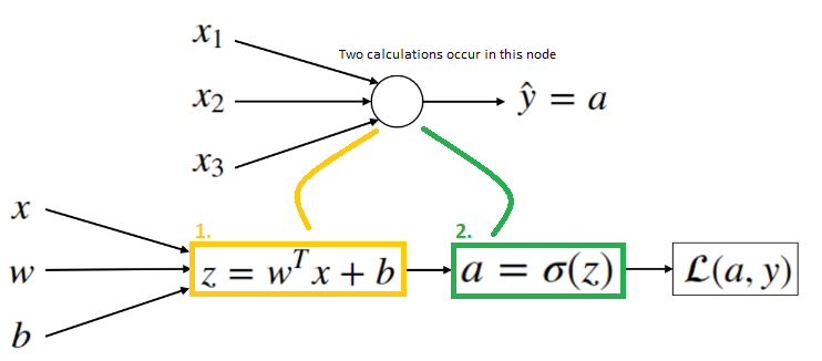
Computing an output of a Neural Network is like computing an output in Logistic Regression, but repeating it multiple times. We have said that circle in Logistic Regression, or one node in Neural Network, represents two steps of calculations. We have also said that Logistic Regression is the simplest Neural Network. So if we have, for

Now we will see how we can compute the output of this simplest neural network.
From the code we have presented above we can see that Logistic Regression doesn’t work well on datasets which are not linearly separable, so we need a deeper representation of a neural network.
We will show how to compute the output of the following neural network
If we look at the first node and write equations for that node, and the same we will do with the second node.
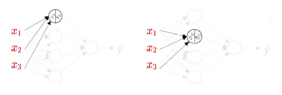
\(\color{Green} {z_1^{[1]} } = \color{Orange} {w_1^{[1]}} ^T \color{Red}x + \color{Blue} {b_1^{[1]} } \enspace \enspace \enspace \enspace \enspace \enspace \enspace \enspace \enspace \enspace \enspace \enspace \color{Green} {z_2^{[1]} } = \color{Orange} {w_2^{[1]}} ^T \color{Red}x + \color{Blue} {b_2^{[1]} } \)
\(\color{Purple} {a_1^{[1]}} = \sigma( \color{Green} {z_1^{[1]}} ) \enspace \enspace \enspace \enspace \enspace \enspace \enspace \enspace \enspace \enspace \enspace \enspace \color{Purple} {a_2^{[1]}} = \sigma( \color{Green} {z_2^{[1]}} ) \)
Calculations for the third and fourth node look the same. Now, we will put all these equations together:
\(\color{Green} {z_1^{[1]} } = \color{Orange} {w_1^{[1]}} ^T \color{Red}x + \color{Blue} {b_1^{[1]} }\) \(\color{Purple} {a_1^{[1]}} = \sigma( \color{Green} {z_1^{[1]}} ) \)
\(\color{Green} {z_2^{[1]} } = \color{Orange} {w_2^{[1]}} ^T \color{Red}x + \color{Blue} {b_2^{[1]} }\) \(\color{Purple} {a_2^{[1]}} = \sigma( \color{Green} {z_2^{[1]}} ) \)
\(\color{Green} {z_3^{[1]} } = \color{Orange} {w_3^{[1]}} ^T \color{Red}x + \color{Blue} {b_3^{[1]} }\) \(\color{Purple} {a_3^{[1]}} = \sigma( \color{Green} {z_3^{[1]}} ) \)
\(\color{Green} {z_4^{[1]} } = \color{Orange} {w_4^{[1]}} ^T \color{Red}x + \color{Blue} {b_4^{[1]} }\) \(\color{Purple} {a_4^{[1]}} = \sigma( \color{Green} {z_4^{[1]}} ) \)
Calculating all these equations with \(for \) loop is highly inefficient so we will need to vectorize this.
\begin{equation} \begin{bmatrix} \color{Orange}- & \color{Orange} {w_1^{[1]} }^T & \color{Orange}-\\ \color{Orange}- & \color{Orange} {w_2^{[1] } } ^T & \color{Orange}- \\ \color{Orange}- & \color{Orange} {w_3^{[1]} }^T & \color{Orange}- \\ \color{Orange}- & \color{Orange} {w_4^{[1]} }^T & \color{Orange}- \end{bmatrix} \begin{bmatrix} \color{Red}{x_1} \\ \color{Red}{x_2} \\ \color{Red}{x_3} \end{bmatrix} + \begin{bmatrix} \color{Blue} {b_1^{[1]} } \\ \color{Blue} {b_2^{[1]} } \\ \color{Blue} {b_3^{[1]} } \\ \color{Blue} {b_4^{[1]} } \end{bmatrix} = \begin{bmatrix} \color{Orange} {w_1^{[1]} }^T \color{Red}x + \color{Blue} {b_1^{[1]} } \\ \color{Orange} {w_2^{[1] } } ^T \color{Red}x +\color{Blue} {b_2^{[1]} } \\ \color{Orange} {w_3^{[1]} }^T \color{Red}x +\color{Blue} {b_3^{[1]} } \\ \color{Orange} {w_4^{[1]} }^T \color{Red}x + \color{Blue} {b_4^{[1]} } \end{bmatrix} = \begin{bmatrix} \color{Green} {z_1^{[1]} } \\ \color{Green} {z_2^{[1]} } \\ \color{Green} {z_3^{[1]} } \\ \color{Green} {z_4^{[1]} } \end{bmatrix} \end{equation}
So we can define these matrices:
| \(\color{Orange}{W^{[1]}} = \begin{bmatrix} \color{Orange}- & \color{Orange} {w_1^{[1]} }^T & \color{Orange}-\\ \color{Orange}- & \color{Orange} {w_2^{[1] } } ^T & \color{Orange}- \\ \color{Orange}- & \color{Orange} {w_3^{[1]} }^T & \color{Orange}- \\ \color{Orange}- & \color{Orange} {w_4^{[1]} }^T & \color{Orange}- \end{bmatrix} \) | \(\color{Blue} {b^{[1]}} = \begin{bmatrix} \color{Blue} {b_1^{[1]} } \\ \color{Blue} {b_2^{[1]} } \\ \color{Blue} {b_3^{[1]} } \\ \color{Blue} {b_4^{[1]} } \end{bmatrix} \) |
| \( \color{Green} {z^{[1]} } = \begin{bmatrix} \color{Green} {z_1^{[1]} } \\ \color{Green} {z_2^{[1]} } \\ \color{Green} {z_3^{[1]} } \\ \color{Green} {z_4^{[1]} } \end{bmatrix} \) | \( \color{Purple} {a^{[1]} } = \begin{bmatrix} \color{Purple} {a_1^{[1]} } \\ \color{Purple} {a_2^{[1]} } \\ \color{Purple} {a_3^{[1]} } \\ \color{Purple} {a_4^{[1]} } \end{bmatrix} \) |
To compute the output of a Neural Network we need the following four equations. For the first layer of a Neural network we need these equations:
\(\color{Green}{z^{[1]} } = W^{[1]} x + b ^{[1]}\)
\(dimensions\enspace are: (4,1) = (4,3)(3,1) + (4,1) \)
\(\color{Purple}{a^{[1]}} = \sigma (\color{Green}{ z^{[1]} }) \)
\(dimensions \enspace are: (4,1) = (4,1) \)
and for the second:
\(\color{YellowGreen}{z^{[2]} } = W^{[2]} x + b ^{[2]} \)
\(dimensions\enspace are: (1,1) = (1,4)(4,1) + (1,1) \)
\(\color{Pink}{a^{[2]}} = \sigma ( \color{LimeGreen}{z^{[2]} }) \)
\(dimensions\enspace are: (1,1) = (1,1) \)
Calculating the output of the Neural Network is like calculating a Logistic Regression with parameters \( W^{[2]} \) as \(w^T \) and \( b ^{[2]} \) as \(b \).
In the next post, we will learn about Shallow Neural Networks.