#010A Gradient Descent for Neural Networks
In this post we will see how to implement gradient descent for one hidden layer Neural Network as presented in the picture below.

One hidden layer Neural Network
Parameters for one hidden layer Neural Network are \(\textbf{W}^{[1]} \), \(b^{[1]} \), \(\textbf{W}^{[2]} \) and \(b^{[2]} \). Number of unitis in each layer are:
- input of a Neural Network is feature vector ,so the length of “zero” layer \(a^{[0]} \) is the size of an input feature vector \(n_{x} = n^{[0]} \)
- number of hidden units in a hidden layer is \(n^{[1]} \)
- number of units in output layer is \(n^{[2]}\), so far we had one unit in an output layer so \(n^{[2]} \)
As we have defined a number of units in hidden layers we can now tell what are dimension of the following matrices:
- \(\textbf{W}^{[1]} \) is \((n^{[1]} , n^{[0]} ) \) matrix
- \(b^{[1]} \) is \((n^{[1]} , 1 ) \) matrix or a column vector
- \(\textbf{W}^{[2]} \) is \((n^{[2]} , n^{[1]} ) \) matrix
- \(b^{[2]} \) is \((n^{[2]} , 1 )\) , so far \(b^{[2]} \) is a scalar
Notation:
- Superscript \([l]\) denotes a quantity associated with the \(l^{th}\) layer.
- Example: \(a^{[L]}\) is the \(L^{th}\) layer activation. \(\textbf{W}^{[L]}\) and \(b^{[L]}\) are the \(L^{th}\) layer parameters.
- Superscript \((i)\) denotes a quantity associated with the \(i^{th}\) example.
- Example: \(x^{(i)}\) is the \(i^{th}\) training example.
- Lowerscript \(i\) denotes the \(i^{th}\) entry of a vector.
- Example: \(a^{[l]}_i\) denotes the \(i^{th}\) entry of the \(i^{th}\) layer’s activations.
Equations for one example \(x^{(i)} \) :
\(z^{[1] (i)} = \textbf{W}^{[1]} x^{(i)} + b^{[1]} \)
\(a^{[1] (i)} = \tanh(z^{[1] (i)}) \)
\(z^{[2] (i)} = \textbf{W}^{[2]} a^{[1] (i)} + b^{[2]} \)
\(\hat{y}^{(i)} = a^{[2] (i)} = \sigma(z^{ [2] (i)}) \)
$$ \hat{y^{(i)}} = \begin{cases} 1 & \mbox{if } a^{[2](i)} > 0.5 \\ 0 & \mbox{otherwise } \end{cases} $$
Assuming that we are doing a binary classification, and assuming that we have \(m \) training examples, the cost function \(J \) is:
\(J (\textbf{W}^{[1]}, b^{[1]}, \textbf{W}^{[2]}, b^{[2]} ) = \frac{1}{m}\sum_{i=1}^{m} \mathcal{L}(\hat{y}^{(i)},y^{(i)}) = \frac{1}{m}\sum_{i=1}^{m} \mathcal{L}(a^{[2](i)},y^{(i)}) \)
\(J = – \frac{1}{m} \sum\limits_{i = 0}^{m} \large{(} \small y^{(i)}\log\left(a^{[2] (i)}\right) + (1-y^{(i)})\log\left(1- a^{[2] (i)}\right) \large{)} \small \)
To train parameters of our algorithm we need to perform gradient descent. When training neural network, it is important to initialize the parameters randomly rather then to all zeros. More about that you can see in this post. So after initializing the paramethers we get into gradient descent which looks like this:
\(repeat \enspace until \enspace convergence: \)
\(calculate \enspace predictions \enspace ( \hat{y}, i\enspace = \enspace 1 .. m ) \)
\(\textbf{dW}^{[1]} = \frac{\partial J}{\partial \textbf{W}^{[1]}} \)
\(db^{[1]} = \frac{\partial J}{\partial db^{[1]}} \)
\(\textbf{dW}^{[2]} = \frac{\partial J}{\partial \textbf{W}^{[2]}} \)
\(db^{[2]} = \frac{\partial J}{\partial db^{[2]}} \)
\(\textbf{W}^{[1]} = \textbf{W}^{[1]} – \alpha \textbf{dW}^{[1]} \)
\(b^{[1]} = b^{[1]} – \alpha db^{[1]} \)
\(\textbf{W}^{[2]} = \textbf{W}^{[2]} – \alpha \textbf{dW}^{[2]} \)
\(b^{[2]} = b^{[2]} – \alpha db^{[2]} \)
So we need equations to calculate these derivatives.
Forward propagation equations (remember that if we are doing a binary classification then the activation function in the output layer is a \(sigmoid\) function):
| Non – Vectorized (for a single training example) | Vectorized |
|
\(z^{[1] (i)} = \textbf{W}^{[1]} x^{(i)} + b^{[1]} \) \(a^{[1] (i)} = \tanh(z^{[1] (i)}) \) \(z^{[2] (i)} = \textbf{W}^{[2]} a^{[1] (i)} + b^{[2]} \) \(\hat{y}^{(i)} = a^{[2] (i)} = \sigma(z^{ [2] (i)}) \) |
\(\textbf{Z}^{[1]} = \textbf{W}^{[1]}X + b^{[1]} \) \(\textbf{A}^{[1]} = \tanh(\textbf{Z}^{[1]}) \) \(\textbf{Z}^{[1]}=\textbf{W}^{[2]}A^{[1]} + b^{[2]} \) \(\textbf{A}^{[2]} = \sigma(\textbf{Z}^{[2]})=\sigma (\textbf{Z}^{[2]}) \) |
Now we will show equations in the backpropagation step:
|
Non – Vectorized \(dz^{[2]} = a^{[2]} – y \) \(\textbf{dW}^{[2]} = dz^{[2]} a^{[1]T} \) \(db^{[2]} = dz^{[2]} \) \(dz^{[1]} = \textbf{W}^{[1]T}dz^{[2]} \ast g’^{[1]}(z^{[1]}) \) \(\textbf{dW}^{[1]} = dz^{[1]} x^{T} \) \(db^{[1]} = dz^{[1]} \) |
Vectorized \(\textbf{dZ}^{[2]} = \textbf{A}^{[2]} – \textbf{Y} \) \(\textbf{dW}^{[2]} = \textbf{dZ}^{[2]} \textbf{A}^{[1]T} \) \(db^{[2]} = \frac{1}{m} np.sum(\textbf{dZ}^{[2]}, axis = 1, keepdims=True ) \) \(\textbf{dZ}^{[1]} = \textbf{W}^{[1]T}\textbf{dZ}^{[2]} \ast g’^{[1]}(\textbf{Z}^{[1]}) \) \(\textbf{dW}^{[1]} = \frac{1}{m} \textbf{dZ}^{[1]}\textbf{X}^{T} \) \(db^{[1]} = \frac{1}{m}np.sum(\textbf{dZ}^{[1]}, axis=1, keepdims = True ) \) |
Sign \(*\) stands for element wise multiplication.
We will now the relation between a computation graph and these equations.
When we talked about Logistic Regression we had forward pass where we computed values of \(z \), \(a \) and at the end the loss \(\mathcal L\). Then we had backward pass for calculating the derivatives, so we computed \(da \), \(dz \), and then \(dw \) , \(db \). Let’s see now the graph for Logistic Regression.
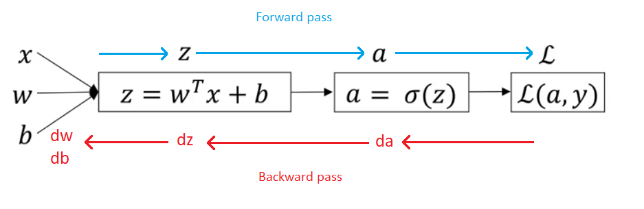
Computation graph for Logistic Regression
We have defined a loss function the actual loss when the ground truth label is \(y \), and our output is \(a\):
\( \mathcal L(a = \hat{y},y) =- \enspace y loga-(1-y) \enspace log(1-a) \enspace \)
And corresponding derivatives are:
\(da = -\frac{y}{a} + \frac{1-y}{1-a} \)
\(dz = da g'(z) \enspace if \enspace g(z) = \sigma(z) = a \enspace \Rightarrow \enspace\)
\(dz =(-\frac{y}{a} + \frac{1-y}{1-a} )a(1-a) = a-y \)
\(dw = dz \enspace x \)
\(db = dz \)
Backpropagation graph for one hidden layer Neural Network
Backprpagation grapf is a graph that describes which calculations do we need to make when we want to calculate various derivatives and do the parameters update. In the following graph we can see that it is similar to the Logistic Regression grapf except that we do those calculations twice.
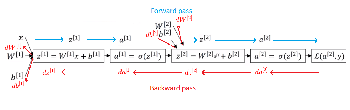
Computation graph for 2 – layer Neural Network
Backpropagation algorithm is a technique used in training neural networks to update the weights and biases by calculating the gradient so that the accuracy of the neural network can be improved iteratively.
Firstly, we calculate \(da^{[2]}\) , \(dz^{[2]}\) and these calculations allows us to calculate \(\textbf{dW}^{[2]}\) and \(db^{[2]}\). Then, as we go deeper in the backpropagation step, we calculate \(da^{[1]}\) , \(dz^{[1]}\) which allows us to calculate \(\textbf{dW}^{[1]}\) and \(db^{[1]}\). If you are interested in how these derivatives are calculated check these notes.
Click here to see how we can implement these ideas in Python.
In the next post we will learn how to train a shallow neural network with Gradient Descent.