🎯 What You’ll Learn

In this comprehensive guide, we’ll explore a unified framework for understanding deep learning architectures across different data types. You’ll learn how to design models based on fundamental principles of invariance and equivariance, understand the spectrum from domain-specific to general-purpose approaches, master the building blocks of temporal sequence models including RNNs and Transformers, and discover how spatial convolution models and graph neural networks all fit into one coherent paradigm. By the end, you’ll have both the theoretical foundation and practical knowledge to approach any deep learning architecture challenge with confidence.

The Domain-Specific to General-Purpose Spectrum

Any AI model you design will probably fit somewhere within a continuum, ranging from highly domain-specific methods that deeply incorporate structural knowledge and expert insights about your particular problem, to more general-purpose approaches that rely heavily on data and computation while requiring less specialized domain understanding.

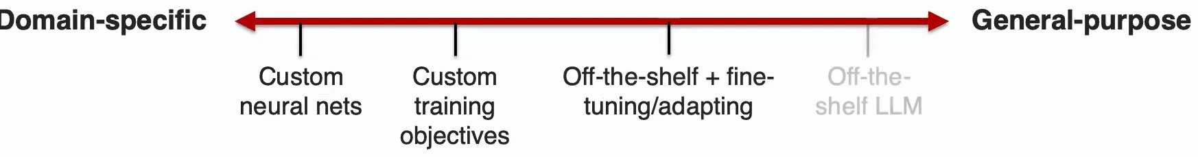
Domain-Specific Approaches: On one end of this spectrum, you might find yourself designing custom neural network architectures with very specialized structures tailored to your specific use case. This could involve creating custom training objectives that embed particular knowledge you have about the problem or enforce certain properties that you know your data should exhibit.

General-Purpose Approaches: Moving toward the other end, you’ll encounter approaches like taking off-the-shelf models and either applying them directly – which would be the most general-purpose approach – or performing some fine-tuning and adaptation of these pre-trained models to better suit your specific needs.

💡 Understanding Model Requirements

Once you understand where your problem sits on the modeling spectrum, the next step is determining what makes a model truly effective for your specific application. A good model should:

• Capture the right semantic information – Whether you’re making predictions, generating data with certain properties, or performing forecasting
• Work at appropriate granularity – Some problems require fine-grained localization while others need high-level summaries
• Use appropriate amounts of data and labels – Different points on the spectrum require fundamentally different amounts of both unlabeled and labeled data
• Respect resource constraints – Some models are more suitable for large GPUs while others work better on edge devices
• Provide the right usability level – Including interpretability and accessibility features that help explain the model’s decisions

🔴 Critical Design Question

Before you start designing your model, ask yourself: What are the properties that are good to have, and what are the ones you absolutely cannot compromise on? This fundamental question should guide every subsequent architecture decision.

The Modality Profile Concept

Every dataset you collect and every task you’re trying to model has certain characteristics that you need to break down systematically. For each characteristic, you need to understand how to model it from your data:

• Elements and their representations – What are the basic units of your data?
• Distribution of elements – Are you looking at sparse regions or high-frequency data?
• Structure – Is it spatial, graphical, sequential, or something else?
• Types of noise – What noise should your model be robust to?
• Relevance – How relevant is each aspect for your specific task?

After you’ve understood your data by breaking it down into individual elements, their composition, distribution, and other characteristics, you can start building your deep learning model. This foundational step sets the stage for how your model will process and understand the data patterns relevant to your specific application domain.

Learning Representations: The Foundation

Learning representations is fundamentally about taking high-dimensional raw data and transforming it into more abstract features that extract meaningful information. There’s going to be some auto-encoder that essentially transforms this into denser, lower-dimensional features while capturing the important information from your data.

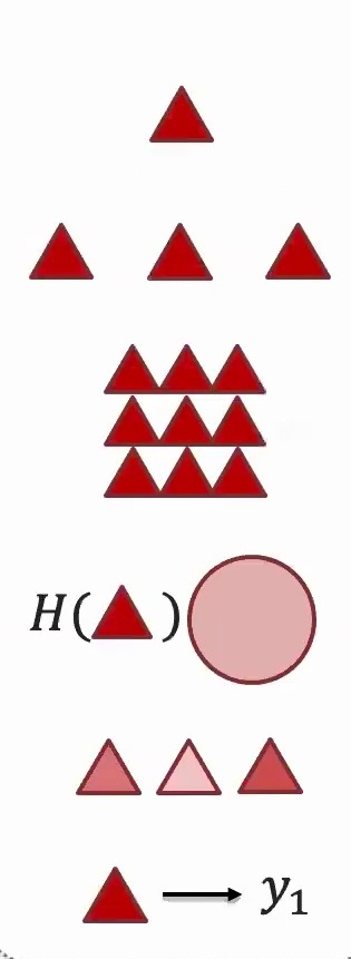
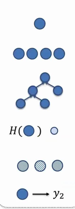
This process is crucial because it allows us to work with more manageable and informative representations rather than the overwhelming complexity of raw input. Different modalities (like the triangular and circular elements shown above) may require different representation strategies, but they all follow this same fundamental principle.

💡 Combining Representations

A second key property in almost all deep learning models is that of combining representations. You might have a representation for the plane in an image, your representation for the sky, your representation for the ground with houses on top of it – all those are representations that represent some meaning. But how do you combine them to learn the information in the holistic scene?

Deep learning is always alternating between steps of extracting features and learning representations, then combining these features later and later as you go deeper into the model to learn more informative and summarized representations.

Building Blocks for Learning Representations

When building deep learning models, it’s crucial to understand that if you have too many linear functions, you’re just going to end up learning a linear model. This is why we need several key components:

• Fully Connected Networks – Basically matrix multiplications that transform your data
• Non-linear Activation Functions (ReLU) – Allow you to start approximating more complicated functions. In fact, you can prove that in the limit, neural networks can express essentially any function
• Layer Normalization – Helps standardize your data and make everything into a nice normalized range
• Convolution – Essential for spatial feature extraction
• Self-Attention – Critical for understanding relationships between different parts of your data

🔴 Why Non-Linearity Matters

If everything were linear with just fully connected layers, those would be linear functions. This is precisely why we need non-linear activation functions to capture more complex patterns and relationships in the data. Without them, stacking multiple layers would be mathematically equivalent to having just one layer!

Blocks for Information Aggregation

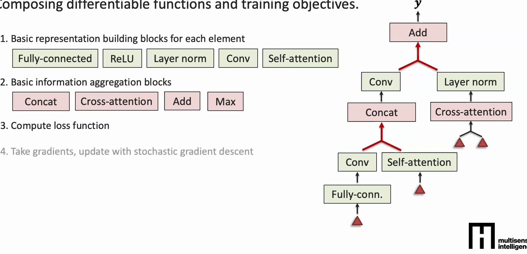
If you have features learned from one part of an image, how do you combine them with features from other parts to learn a representation for the whole image? There are several approaches:

• Concatenation – A very simple way of combining information by stacking features together
• Attention Mechanisms – Dynamically weight different parts of your input
• Pointwise Addition – Simply add corresponding elements from two vectors
• Pointwise Max – Take the maximum between corresponding elements of two vectors

These aggregation methods allow you to combine local information into increasingly global representations as you move deeper into the network.

The Unified View

A unified view of deep learning models shows that these models always have several key steps, with learning representations being the foundational one. Every deep learning architecture – whether it’s a CNN, RNN, Transformer, or Graph Neural Network – can be understood through this lens of:

1. Learning representations from raw data
2. Combining these representations hierarchically
3. Repeating this process through multiple layers to capture increasingly abstract patterns

💡 Set-Based Data Classification

Imagine you have a set of five images representing different objects. Your goal is to classify this collection – perhaps determining which image is the anomalous one, or deciding if this particular set depicts outdoor versus indoor scenes.

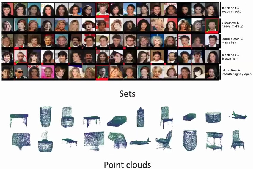
The key challenge: The classification should not depend on the order in which we present these images to our model. Whether we show them as A, B, C, D, E or E, C, B, D, A, the model should produce the same result. This is called permutation invariance.

Two Key Architectural Principles for Sets

Almost all successful deep learning models for sets rely on two key architectural principles:

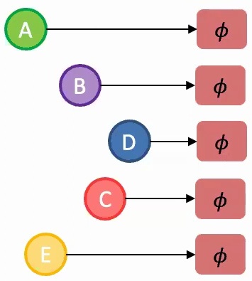
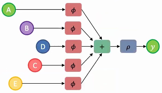
1. Parameter Sharing: You should share parameters across the model components that encode each set element – think of this as using the same parameter file (represented by the same color \(\phi\)) for processing each element A, B, C, D, and E.

2. Permutation-Invariant Aggregation: You need to aggregate the learned information from individual representations using a permutation-invariant function. Element-wise addition works perfectly here since adding vectors maintains permutation invariance.

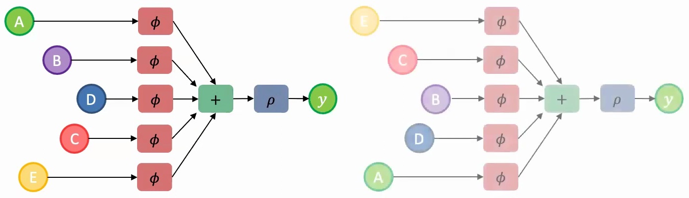
Once you have this aggregated feature representation, you can pass it through additional layers \(\rho\) to make your final predictions. This approach ensures that regardless of whether you present the model with images in order A, B, C, D, E or E, C, B, D, A, the underlying computation and results remain consistent.

🔴 The Cost of Violating These Principles

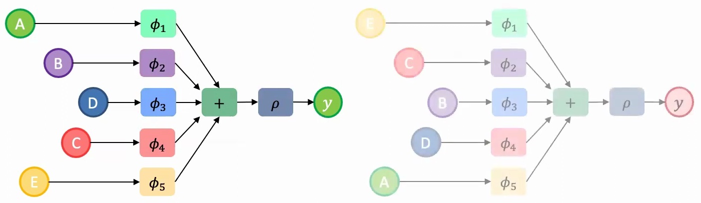
If we don’t use parameter sharing and instead employ different feature extractors \(\phi_1, \phi_2, \ldots, \phi_5\) for each set element, the model will learn vastly different representations for the same set presented in different orders. This means we’d need to train the model on all possible permutations – that’s \(5! = 120\) times more training examples!

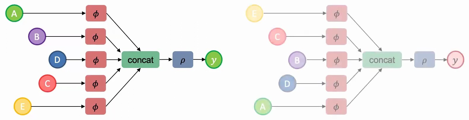
If we use parameter sharing but employ a non-permutation-invariant aggregation function like concatenation instead of addition, we face the same problem since concatenating AB produces a different result than concatenating BA.

Key Insight: Architecture as Prior Knowledge

This analysis generalizes to a fundamental principle in deep learning architecture design: careful architectural choices can dramatically reduce the amount of training data required.

When we design our models to respect the inherent symmetries and invariances in our data – such as permutation invariance for sets – we essentially provide the model with built-in knowledge about the problem structure. This allows the model to generalize from fewer examples, making our learning process both more efficient and more robust.

Understanding Data Invariances

The first key concept is data invariances – these are transformations that you can apply to your data where the label or outcome should not change. Let me give you a concrete example to illustrate this principle.

Imagine you have an image of the digit three, and your goal is to classify what digit it represents. Now, if you move this image up, down, left, or right by a couple of pixels, it should still be classified as a three. Similarly, if you rotate the image by 45 degrees or 90 degrees, or even change it from grayscale to RGB, you should still arrive at the same label of three.

🔴 Why Invariances Matter

This concept of invariances is absolutely crucial for building robust models. Ideally, a model should capture these invariances naturally, because if it doesn’t – if a model is overly sensitive to color changes, rotation, or small shifts in pixel positions left and right – then you’re going to need significantly more training data to learn the same task effectively.

When models fail to understand these fundamental invariances, they essentially treat each slight variation as a completely different input, forcing you to provide examples of every possible transformation rather than learning the underlying structure that makes a three recognizable regardless of these superficial changes.

Invariance vs Equivariance in Vision Tasks

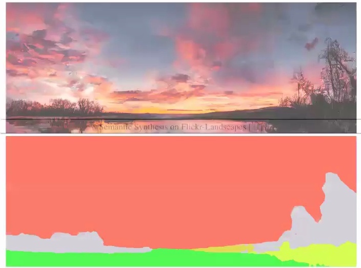
While image classification exemplifies a task where certain invariances exist in your data, we also need to understand equivariances. Invariances are changes to the input where the model should not be sensitive to, which stands in contrast to equivariances. Equivariances are changes in the input data that the model should be sensitive to and respond accordingly.

Consider an image with a digit three on it, where your goal is to create a semantic map – essentially labeling regions as background, digit, tree, ocean, or other semantic categories for segmentation purposes. If you shift this image up by two pixels, your semantic map should correspondingly shift upwards by two pixels. Similarly, if you rotate the image 45 degrees, your semantic map should also rotate 45 degrees.

💡 Practical Examples

In the segmentation context, shifting and rotating are equivariant transformations because whatever change you make to the input data, you want the model to capture that same change in the output.

This contrasts with properties like color, where whether the image is RGB or black and white, you should still obtain the same semantic map. RGB and color variations are something the model should be invariant to, while shift and rotation should be equivariant transformations.

These are fundamental properties you need to consider when working with different types of data. For instance, when classifying data based on sets, you must respect the idea of permutation invariance – meaning you can permute your elements however you want, whether given as ABC or CBA, and the model should produce the same result regardless of the ordering of elements in the set.

Group-Equivariant Function Mappings

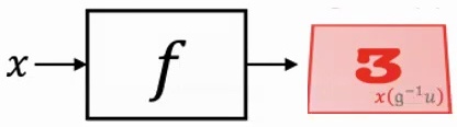
When we talk about group-equivariant function mappings, we’re dealing with a fundamental principle that ensures consistency in how transformations affect both inputs and outputs. The core idea is that applying a group transformation to the input should produce the same result as applying the function first and then transforming the output – this property should ideally not change the output behavior of our model.

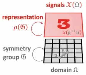
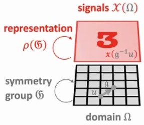
To understand this mathematically, we work with functions \(f\) that map from signal space \(\mathcal{X}(\Omega)\) to itself, where \(\Omega\) represents our domain and \(\mathfrak{G}\) is our symmetry group. The representation \(\rho(\mathfrak{G})\) describes how group elements act on our signals, creating a framework where transformations preserve the essential structure of our data.

💡 Mathematical Formulation

A function \(f : \mathcal{X}(\Omega) \to \mathcal{X}(\Omega)\) is \(\mathfrak{G}\)-equivariant if:

$$f(\rho(g)x) = \rho(g)f(x)$$

for all \(g \in \mathfrak{G}\). This means the group action on the input affects the output in the same way.

This equivariance property is crucial for building robust models that respect the inherent symmetries in our data. When we have a function that satisfies this property for all group elements, we ensure that our model’s behavior remains consistent regardless of how the input is transformed by the group action.

Geometric Deep Learning Framework

Building on these equivariance principles, the geometric deep learning framework provides an elegant way to approach custom architecture design – given your data, you want to create architectures that are both sample-efficient and computationally effective. The key insight is moving beyond ad-hoc design choices toward principled approaches grounded in mathematical structure.

When we examine common architectures through this lens, we can understand why they’re motivated the way they are, essentially mapping mathematical operators to practical building blocks.

🔴 Key Reference

For those interested in diving deeper into this formalization, Bronstein et al.’s paper on geometric deep learning with groups and graphs stands out as probably the best reference. This work rigorously formalizes what’s needed for invariant and equivariant operations – they mathematically define the associated functions needed for permutation invariance and related concepts.

💡 Practical Implementation

However, the beauty of this approach is that it usually doesn’t need to be overly complicated in practice. Often, you can achieve the desired invariances through simple tricks – think about operations like summation or taking element-wise maximum when working with set data.

These straightforward techniques can effectively bake in the mathematical properties you need. So as we move on to explore some common model architectures, keep in mind that they’re all inspired by these fundamental phenomena of invariance and equivariance.

Key Takeaway

The geometric deep learning framework unifies different architectures under common mathematical principles. By understanding group equivariance and invariance, we can design models that are both theoretically sound and practically efficient, requiring less data and computation while maintaining robust performance across transformations.

Elements and Structure of Sequences

You might have some element, for example a word, and this word might constitute part of a longer sequence. So you might have a long sequence of words, or you could have a sequence of time steps in temporal data. These could be various types of data – code, genomics data, or any other sequential information. All of these share the common characteristic of being sequences where the order and relationships between elements matter.

The goal with sequential data is typically to perform some classification task – whether that’s predicting the next word in a sequence, determining some topic, or assigning labels based on the sequential information we’ve observed.

💡 Key Question for Sequential Models

This brings us to the key question: how do you create meaningful representations from this sequential data, and how do you effectively aggregate information across the sequence elements?

Currently, for temporal data processing, a very key idea that emerges is this concept of hierarchical locality. This principle helps us understand how information flows and gets processed within sequential structures, allowing us to build more effective models that can capture both local patterns and longer-range dependencies in our sequential data.

Text Prediction and Classical Models

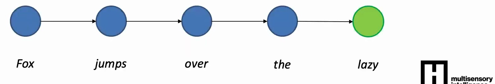
Building on our understanding of sequential structure, when we want to predict the next word in a sequence, it’s natural to consider what comes before it. The word immediately preceding our target is probably going to be the most important factor in making an accurate prediction.

However, we shouldn’t limit ourselves to just the immediate predecessor. It also makes sense to take into account longer context – perhaps the five words before, or even longer range dependencies depending on how much context we can effectively utilize.

🔴 The Core Challenge

The fundamental question we’re addressing is: how do we predict the next word? This challenge really motivates our exploration of classical approaches to sequence modeling, where we learn to balance the importance of immediate context with longer-range dependencies in the text.

Time Series Classification Methods

Intuitively, any model designed for sequential data should be invariant to time itself – whether you obtain a sequence and shift it one step before or after shouldn’t make a big impact on the model’s performance. However, the model should be extremely sensitive to order. For example, if you change “Fox jumps over the dog” to “Dog jumps over the Fox,” that change in word order should significantly affect the model’s output.

💡 Two Key Properties for Sequential Models

To deal with these invariant versus equivariant requirements, almost all models for sequential data incorporate two key properties:

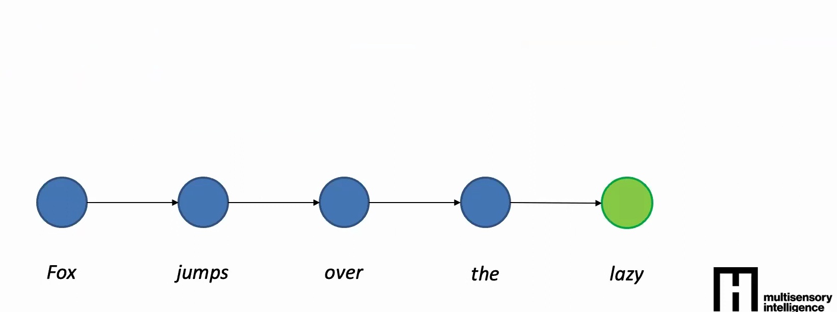
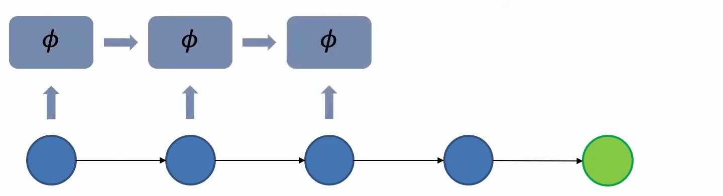
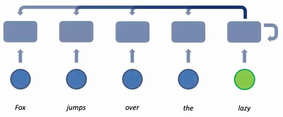
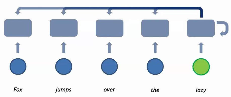
1. Parameter Sharing Across Time Steps: The same model with the same features should process each word in the sequence. Even though the words themselves might be different, the functions you use to process them should be the same. This is critical because otherwise, if you just shift the sequence left or right by a couple of time steps, you’re going to get a very different output without parameter sharing.

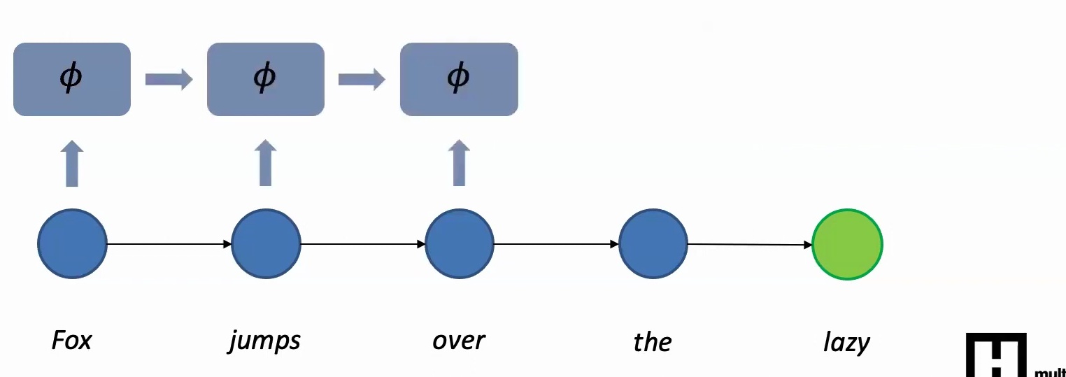
2. Information Aggregation Through Recurrence: You first extract features from the first word, then look at the next word, extract features and accumulate information from the previous word, then extract features from the third word and accumulate what you have from the second and first words, and so on. This idea of information aggregation across time is what makes the model equivariant to word order.

🔴 Critical Design Principle

In summary, models should be insensitive to individual time steps but highly sensitive to the order in which words are presented. The two fundamental ideas are parameter sharing – using the same feature extraction at all time steps – and information aggregation across time in an autoregressive manner. These principles form the foundation for implementing these concepts in neural network architectures.

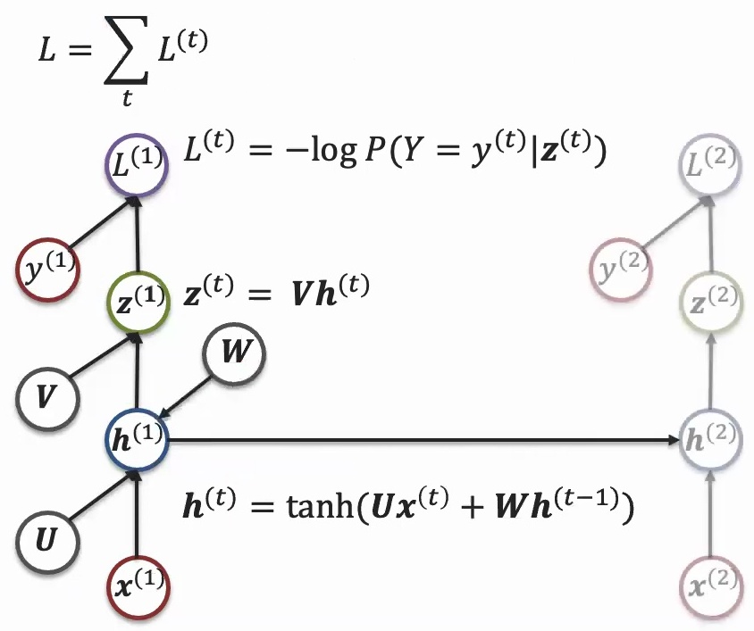
Recurrent Neural Networks for Sequences

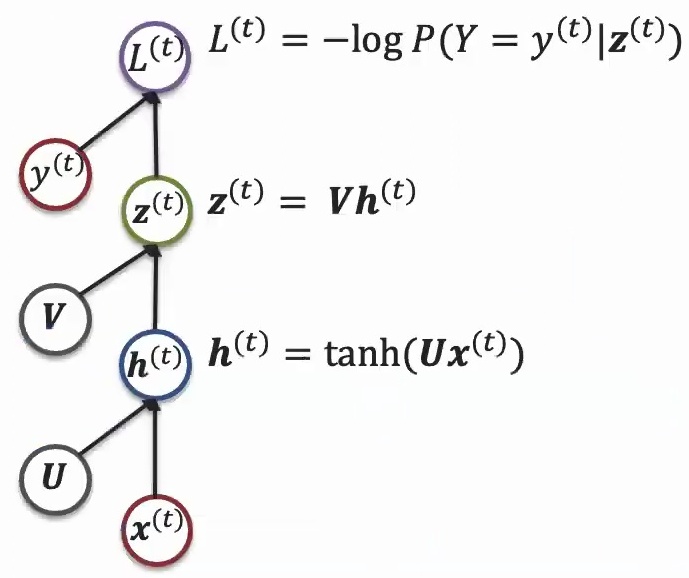
Now let’s see how these theoretical principles translate into concrete neural network architectures. When you have your data \(X\), you apply parameters \(U\) through linear transformations – essentially \(U\) times \(X\) as a matrix multiplication, followed by some activation function like tanh. This allows you to express non-linear functions, and then you might apply a next layer to it with parameter \(V\) times the output from the previous layer. Finally, you compute the loss with respect to the real label – in classification cases, this would be negative log probability.

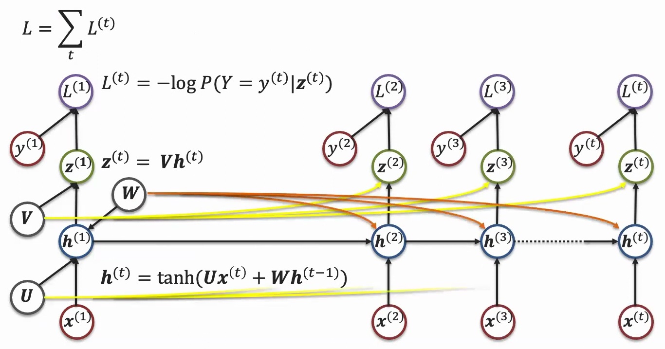
What makes recurrent models special is how they unroll this basic structure across time. The same parameters \(U\) and \(V\) are applied to different time steps in the sequence – \(X_1\), \(X_2\), \(X_3\), and so on. This is the key insight: while the data coming in is different at each time step, the same parameters are applied consistently. This parameter sharing allows information to accumulate across the sequence, creating a memory effect where each time step builds upon the previous ones.

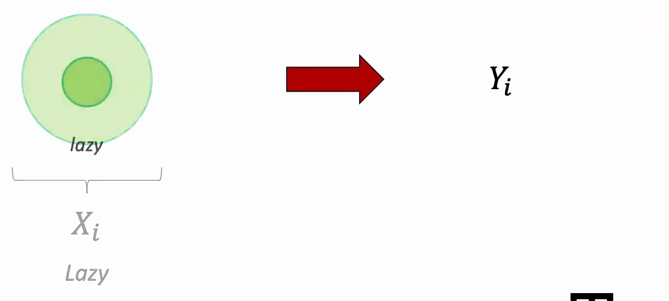
💡 From Classification to Generation

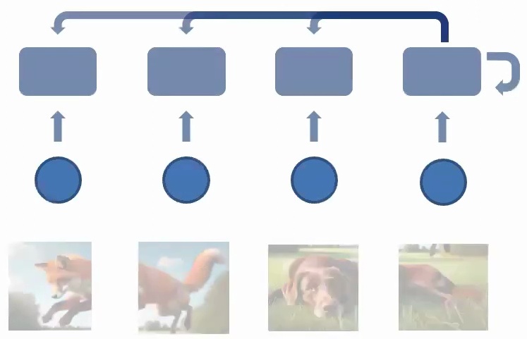
This framework isn’t limited to just sequence classification – you can extend it to sequence generation as well. Instead of having a sequence coming in and predicting a single label, you can take one input and predict multiple outputs.

For example, if I give you the word ‘fox’ and your goal is to complete the story or generate music, you use the same parameters at every time step to generate something, then take what you generated previously (\(Y_1\)) as input into the next step. This creates a generative process where the model builds upon its own outputs.

Key Takeaway

Recurrent neural networks implement the fundamental principles of sequential modeling through parameter sharing and recurrent information aggregation. By maintaining the same weights across time steps while accumulating context, RNNs can be both time-invariant and order-equivariant, making them powerful tools for sequence classification and generation tasks.

Text and Music Generation Models

In these models, we follow an autoregressive approach where we generate \(Y_2\) and then take what we generated in \(Y_2\) as the next step to generate \(Y_3\). The key principle is parameter sharing at every step – there’s one set of parameters \(U\) and \(W\) that are shared across all time steps, and you accumulate information across time by taking what you generated previously and feeding it into the next step.

💡 Evolution of Recurrent Architectures

What some of you might realize is that these are recurrent networks, and you might say these are out of fashion, but I actually promise you otherwise. RNNs have evolved significantly over time – the progression goes:

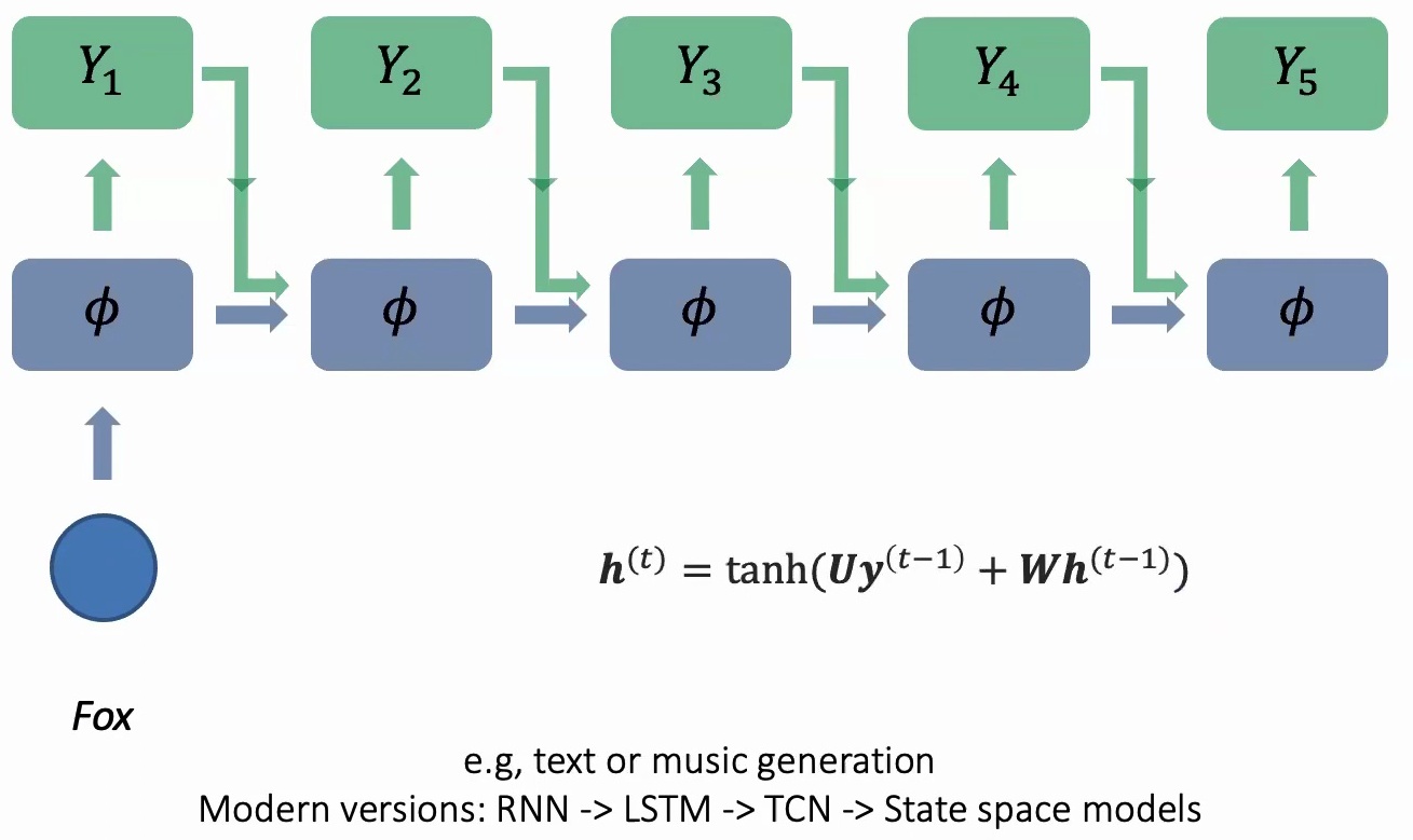
RNN → LSTM → TCN → State space models

RNNs evolved into LSTMs, LSTMs evolved to temporal convolutional networks, and temporal convolutional networks have already inspired a lot of modern work in state-based models, which are still quite popular nowadays if you want to process time series or continuous data as an alternative to transformers.

In sequence-to-sequence models, every feature at your \(t\)-th time step is a function of what you generated at the previous time step and also the hidden features \(h\) at the \(t-1\) previous time step:

$$h^{(t)} = \tanh(Uy^{(t-1)} + Wh^{(t-1)})$$

The parameters \(U\) and \(W\) remain shared across all time steps, maintaining the fundamental principle of parameter sharing that makes these models efficient and effective for sequential data processing.

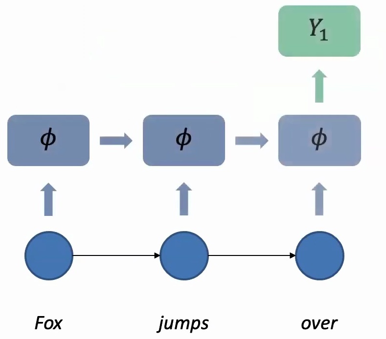
Sequence-to-Sequence Translation

Building on the generation principles we just covered, sequence-to-sequence models operate on a fundamental principle: there’s a sequence coming in and a sequence that comes out. When the input sequence arrives, we apply the same parameters at every time step to process each word, accumulating information across time steps.

You’ll take words like “Fox,” “jumps,” “over,” and accumulate information progressively. Once you finish reading the entire sequence, you can predict the first output \(Y_1\), and then autoregressively take the previous output, feed it into the next step to generate \(Y_2\), then use \(Y_2\) to generate \(Y_3\), and so on.

🔴 The Translation Challenge

These sequence-to-sequence models are extensively used in machine translation, where you want to convert a sentence of three English words into a sentence of three French words. They’re also fundamental to many generative models we use today.

However, translation isn’t straightforward because different languages have different structures – why does one word correspond to “Fox” and another to “jumps”? In some languages, the subject-object relationship might be expressed differently than in others, creating complex mapping challenges between source and target languages.

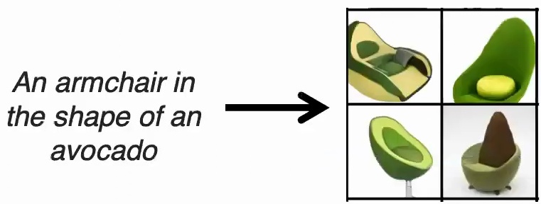
💡 The Birth of Attention Mechanisms

A pivotal breakthrough in machine translation came with the introduction of attention mechanisms, visualized through heat maps that show which English words correspond to which French words in the output.

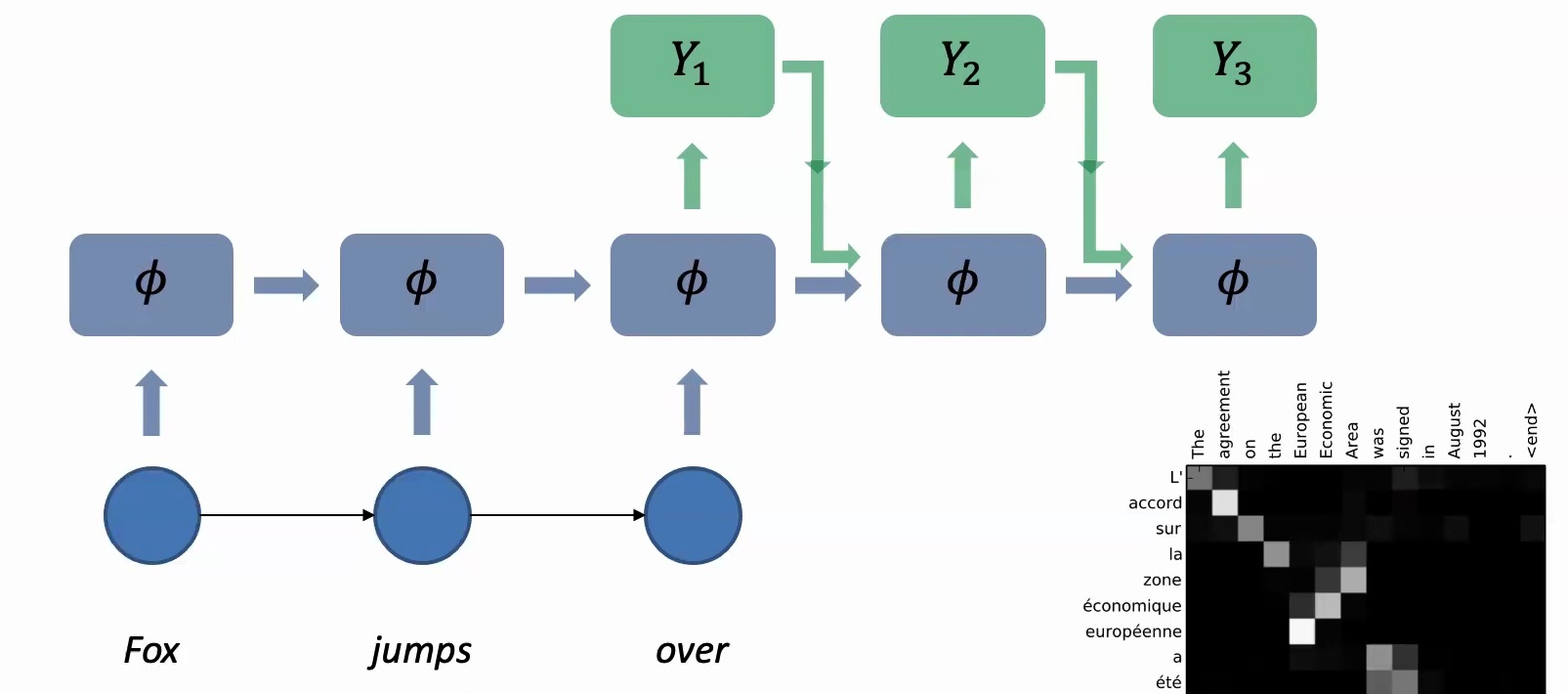
These attention maps reveal fascinating patterns – while many alignments fall on the diagonal indicating preserved word order, several appear off-diagonal, showing that word order often shifts between English and French. When generating \(Y_1\), the attention mechanism determines which of the input words are most relevant – is it purely “Fox” or maybe a combination of “Fox” and “jumps over”?

This creates a matrix of size input sequence length by output sequence length, which could be square for similar languages but becomes increasingly off-diagonal for more different language pairs like English-Chinese or English-Japanese. The attention matrix doesn’t have to be square – it can absolutely be rectangular with dimensions \(T_1\) by \(T_2\), where you might have three English input words but five Chinese output words.

Key Takeaway

Sequence-to-sequence models with attention mechanisms revolutionized machine translation by allowing models to dynamically focus on relevant parts of the input when generating each output token. This attention-based approach became the foundation for modern transformers, with the first transformer paper benchmarked on machine translation tasks.

Attention Mechanisms in Sequence Models

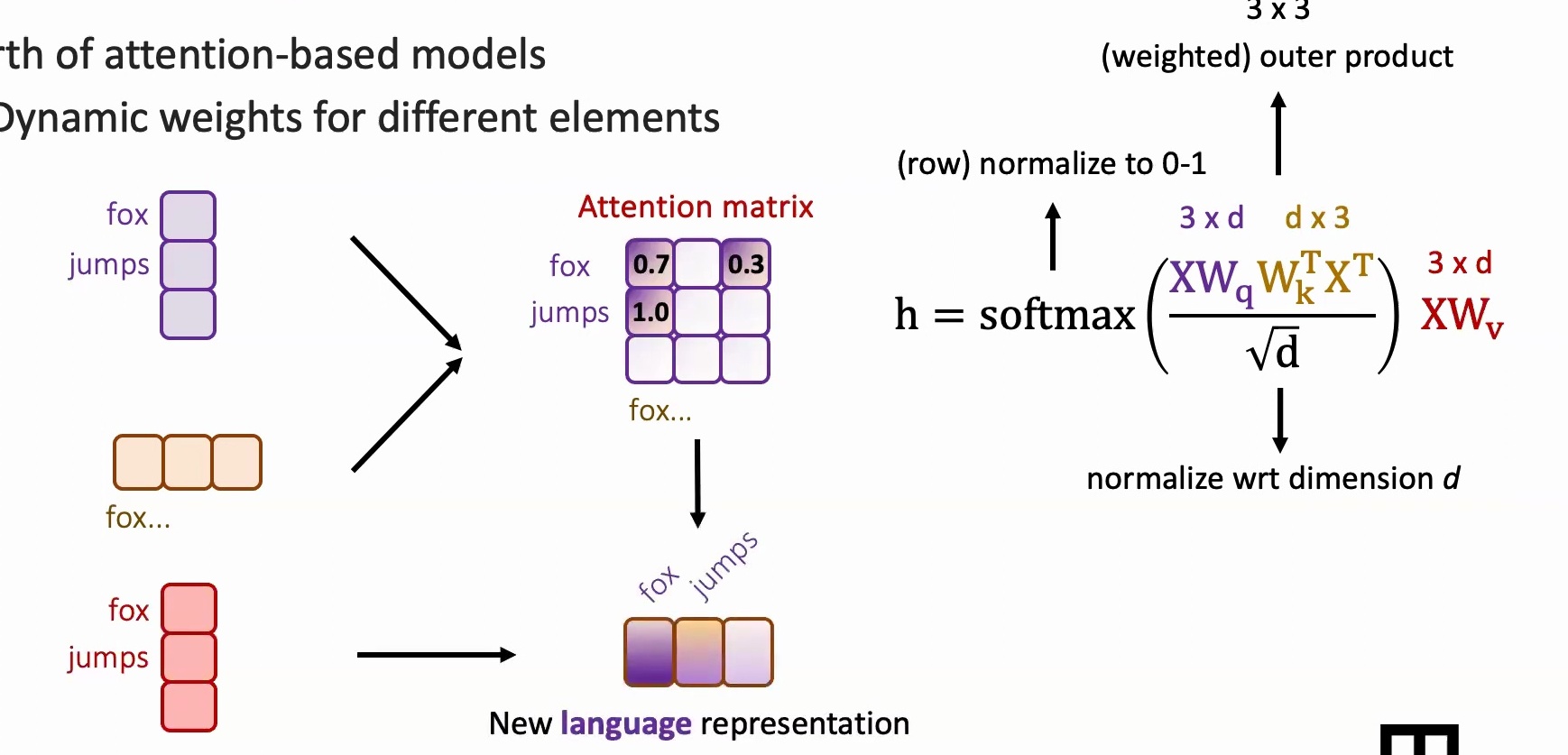
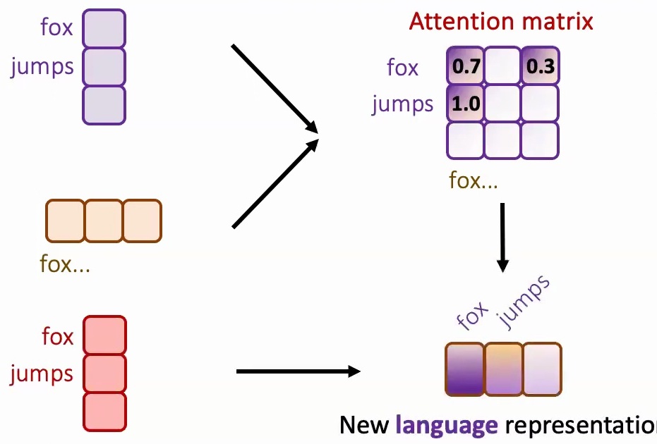
The birth of attention-based models marked a revolutionary shift in sequence modeling, achieving state-of-the-art results across the board. The core idea behind these attention mechanisms is to provide dynamic weights for different elements in a sequence.

When translating text, for example, while processing the first word, the model might focus mostly on that first word but also attend slightly to the second and third words. Similarly, when processing the second word, it looks primarily at the second word while giving some attention to the first and third. This dynamic weighting allows the model to compute new features by leveraging their context in a much more flexible way than traditional approaches.

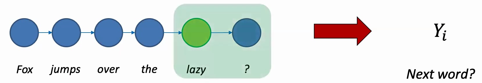
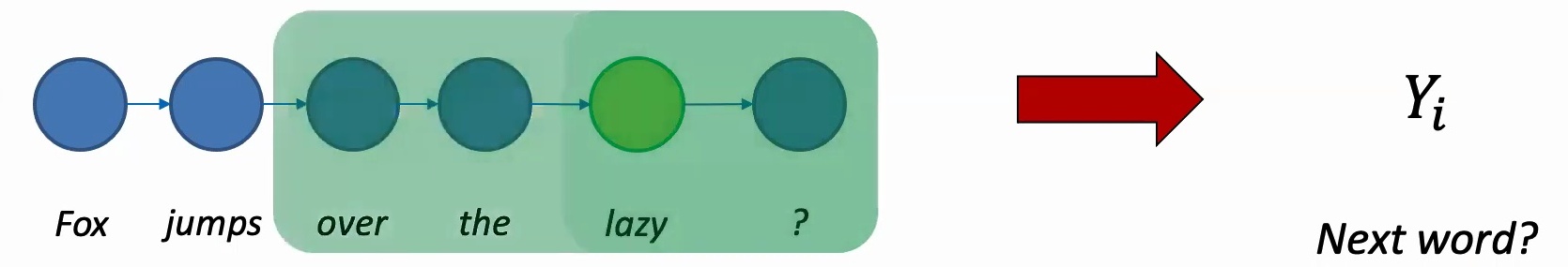
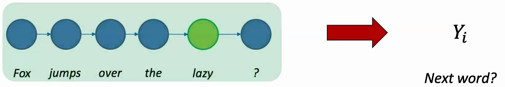
💡 How Attention Scores Work

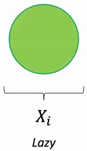
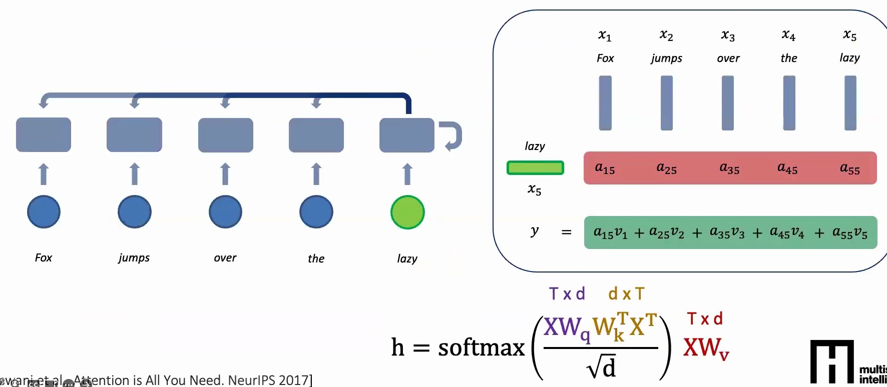
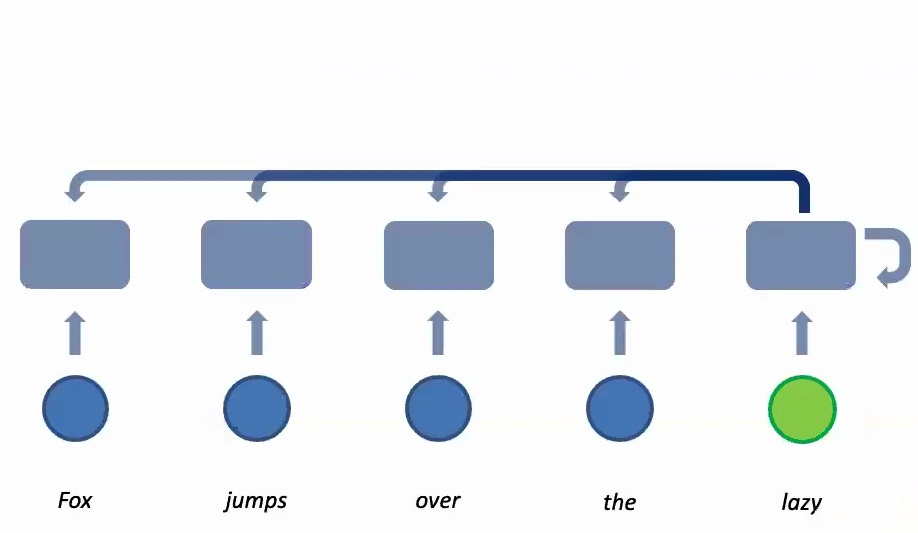
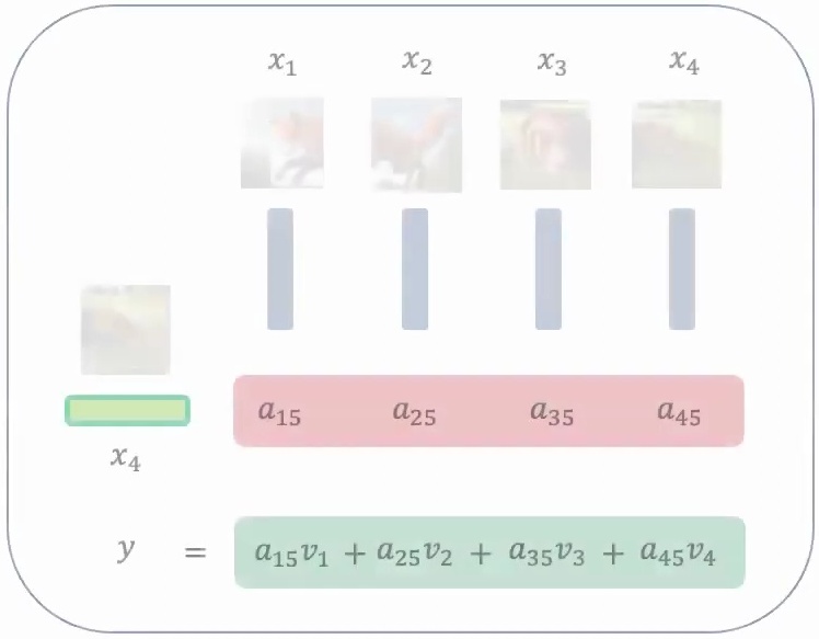
Let me illustrate this with a concrete example. When computing a new feature for the word ‘lazy’ in a five-word sequence, the attention mechanism looks at all four preceding words and computes attention scores \(a_1\) through \(a_5\). These scores tell us how much each of the previous words should contribute to the feature we’re learning for ‘lazy’.

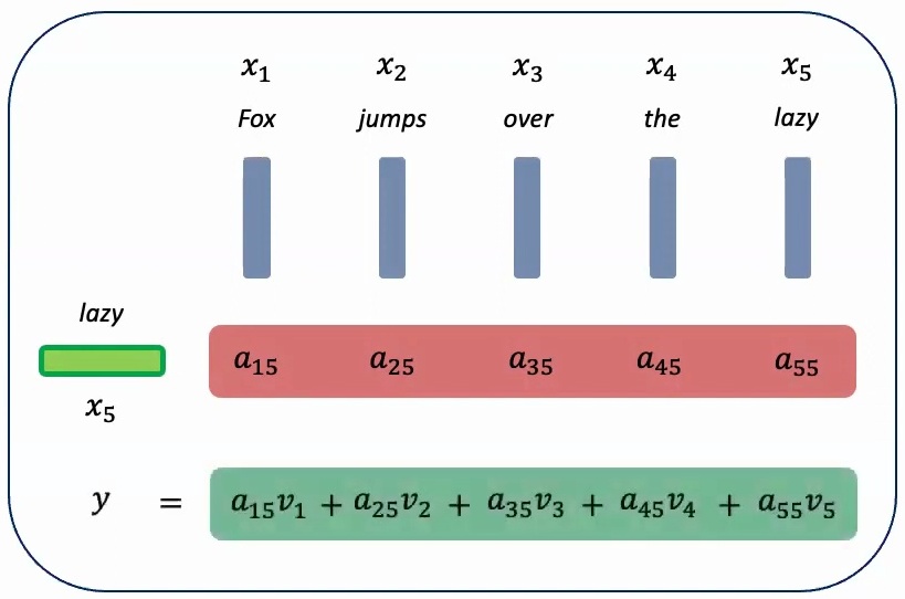
The attention scores represent relative contributions – we might have \(a_1\) times the value of ‘fox’, plus \(a_2\) times the attention given to ‘jumps’, plus \(a_3\) times ‘over’, and so on. Once we obtain these attention scores, we multiply them with the actual features to get a weighted summation, creating a context-aware representation.

The Mathematics of Attention

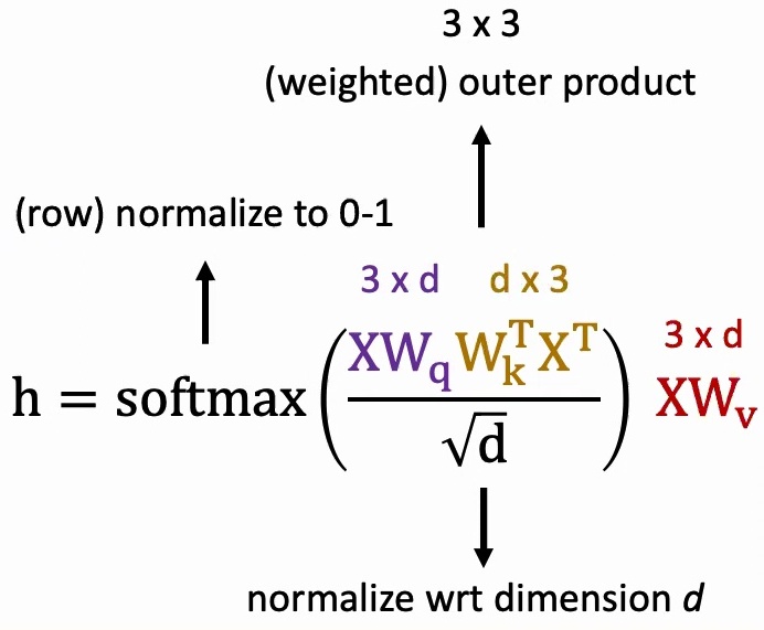
I like to think about attention models abstractly through matrix multiplications, using the equation that everybody has seen in Transformers. Your data \(X\) is essentially \(3 \times D\) – assuming you have three words, each with some \(D\)-dimensional representation.

The query, key, and value matrices are linear transformations that convert your one-hot tokens into lower-dimensional dense features. When we compute \(XW_k^T\), we’re taking the transpose of our \(3 \times D\) data multiplied by another learnable parameter, creating a \(D \times 3\) matrix. This weighted outer product helps us determine, for every one of our three words (say ‘fox’, ‘jumps’, ‘over’), what the pairwise attention scores should be with each other word, resulting in a \(3 \times 3\) attention matrix.

🔴 Critical Implementation Details

The normalization by \(\sqrt{D}\) is crucial because each entry in your \(3 \times 3\) matrix results from a \(D\)-dimensional vector dot product. If \(D\) is large, the magnitude grows quickly, so we normalize by \(\sqrt{D}\) to keep the variance at \(1/D\) and values properly scaled.

After applying softmax row-wise, each row’s entries become non-negative and sum to one, creating a probability distribution. You might see values like \(0.7, 0.3\) or \(1.0, 0.0, 0.0\) – these represent how much attention to focus on each position.

Finally, we multiply this \(3 \times 3\) attention matrix with our feature matrix \(XW_v\) (which is \(3 \times D\)) to get our final \(3 \times D\) output. This output gives us a new representation where each word’s feature incorporates information from all other words, weighted by their attention scores.

Transformer Architectures

Building on these attention mechanisms, let’s return to our unified framework for understanding transformer architectures. When working with sequential data, any model must respect two fundamental properties: invariance to time and equivariance to word order.

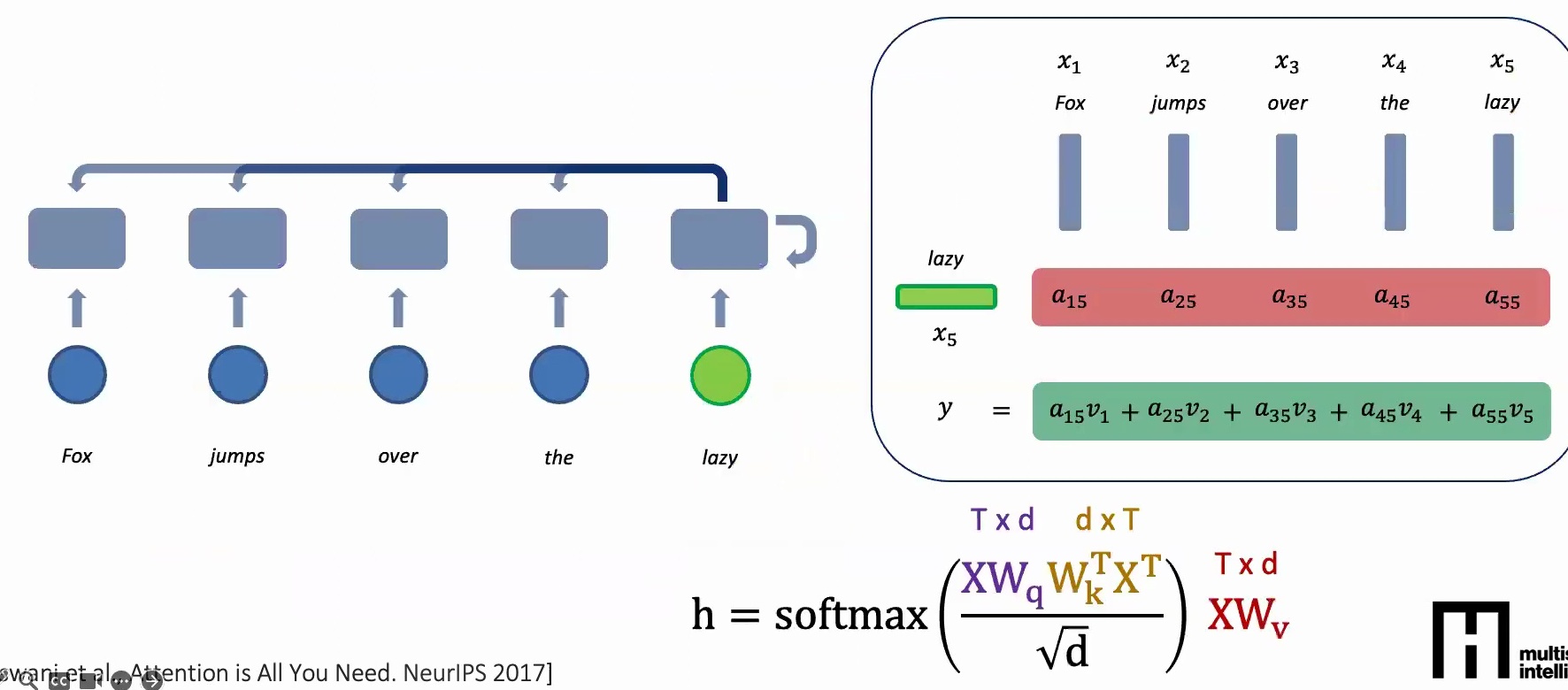
The transformer architecture elegantly maintains both of these critical properties through its design. First, we achieve parameter sharing across time steps – each word that enters the system gets embedded through the same transformer using identical learnable transformations with weight matrices \(W_q\), \(W_k\), and \(W_v\). These three sets of weight matrices are repeated across time, creating the parameter sharing that allows the model to be invariant to time shifts.

This parameter sharing mechanism ensures that whether you shift the sequence back and forth, or pad it with zeros from the left or right, the model will still produce consistent outputs.

💡 Parallel Processing Advantage

The beauty of the transformer lies in how it handles information aggregation differently from traditional sequential models. Instead of processing information sequentially, which can be slower on GPUs, the transformer performs information aggregation in parallel using matrix multiplication.

The model computes the entire attention weight matrix – say a five by five matrix for a sequence of five words – and performs all attention computations in one parallel operation. This parallel processing is what makes transformers so efficient on modern hardware.

Crucially, the model remains equivariant to word order because if you permute the input sequence, the attention patterns change accordingly, and the output will reflect those changes. This maintains the essential property that word order matters while allowing for efficient parallel computation.

Key Takeaway

Transformers revolutionized sequence modeling by replacing sequential recurrence with parallel attention mechanisms. By computing all attention weights simultaneously through matrix operations, transformers achieve both computational efficiency and the ability to capture long-range dependencies, while maintaining the fundamental properties of time invariance and order equivariance through clever use of parameter sharing and attention-based aggregation.

Feature Learning and Data Analysis

The key question becomes how to build a model that can break down the individual elements of an image, learn specific features for each localized region, and then combine information from these local parts to extract increasingly comprehensive insights from the overall image.

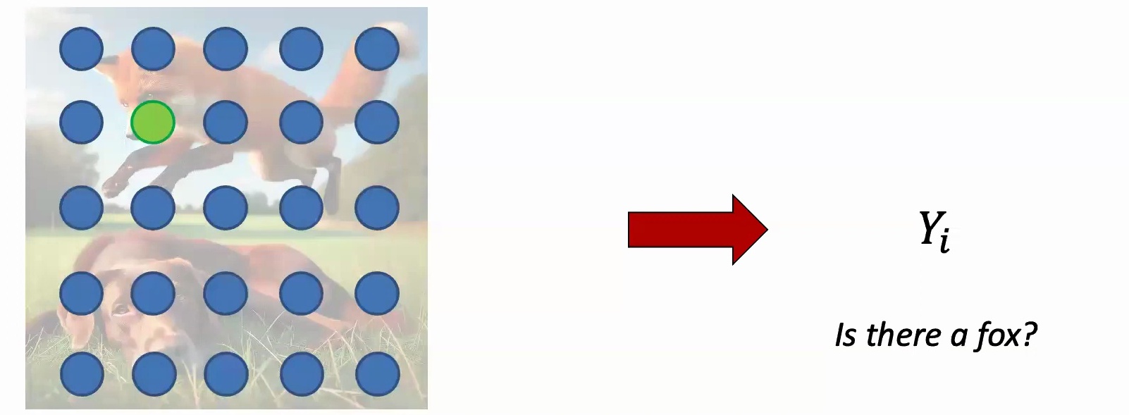
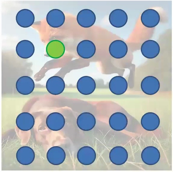
One naive approach to this problem is to systematically sample the image using a grid-based method. By overlaying a regular pattern of sampling points across the spatial data, we can extract features from specific locations and begin to understand the local characteristics of different regions within the image.

This systematic approach allows us to define specific prediction tasks, such as determining whether particular objects or features are present in different regions of the spatial data. By analyzing the sampled points and their corresponding features, we can build models that not only identify local patterns but also understand the broader spatial relationships that exist across the entire dataset.

Data Flattening and Spatial Invariance

Building on our feature extraction approach, let’s examine what happens when we process image data through traditional network architectures. One common approach is to flatten the pixel structure into a sequence that can be processed by fully connected networks.

If you just flatten it, usually these are pixels, and you can flatten it into a sequence of pixels to connect with the next layer for tasks like classification. However, this flattening approach has important implications for spatial invariance – when you’re trying to do classification, the network will probably be very invariant to spatial locations, meaning it doesn’t care much about where features appear in the image.

💡 Task-Dependent Spatial Sensitivity

The choice of spatial sensitivity depends heavily on your specific task:

For Classification: If you’re trying to do classification, you will probably be very invariant to spatial locations. If it’s just to classify something as red and white blocks, then you could rotate all you want without affecting the outcome.

For Segmentation: If you’re trying to do segmentation, you will be sensitive to spatial locations, so the model should be equivariant to any sense of locations. When precise spatial information is required, rotation invariance becomes problematic.

In general, most of these models for images, especially those designed for classification or detection tasks, are going to be very invariant to spatial transformations. This invariance is often desirable for recognition tasks but can be problematic when precise spatial information is required for the application.

🔴 Critical Design Question

Before choosing your architecture, ask yourself: Does my task require spatial equivariance (like segmentation) or spatial invariance (like classification)? This fundamental distinction will guide whether you need models that preserve spatial relationships or models that abstract away from specific locations.

CNN Architecture and Core Principles

Convolutional Neural Networks represent one of the most successful approaches to spatial data processing. CNNs achieve spatial invariance through two fundamental mechanisms that mirror the principles we’ve discussed for sequential data: parameter sharing and hierarchical information aggregation.

Just as we saw with sequential models where the same parameters process each word in a sequence, CNNs apply the same convolutional filters across all spatial locations in an image. This parameter sharing means that whether a feature (like an edge or a corner) appears in the top-left or bottom-right of an image, the same learned filter will detect it, making the model translation-invariant.

The key insight is that CNNs learn a small set of filters (typically \(3 \times 3\) or \(5 \times 5\) pixels) and slide these filters across the entire image. Each filter looks for a specific pattern – one might detect vertical edges, another horizontal edges, another circular shapes, and so on. By sharing these filter parameters across all spatial locations, CNNs dramatically reduce the number of parameters needed compared to fully connected networks.

💡 Sparse Connectivity and Local Receptive Fields

Another crucial property of CNNs is sparse connectivity. Unlike fully connected layers where every input connects to every output, convolutional layers only connect each output to a small local region of the input – the receptive field.

For example, when processing a \(224 \times 224\) image, a \(3 \times 3\) convolutional filter only looks at 9 pixels at a time to compute each output value. This sparse connectivity has several advantages:

• Fewer parameters: Dramatically reduces the number of weights to learn
• Computational efficiency: Less computation per layer
• Better generalization: Reduces risk of overfitting
• Local pattern detection: Naturally captures local spatial relationships

The receptive field grows as you stack more convolutional layers. While the first layer might only see \(3 \times 3\) pixels, the second layer effectively sees a larger region of the original image, and by the time you reach deeper layers, neurons can integrate information from much larger spatial regions while maintaining the efficiency of local operations.

Hierarchical Feature Learning in CNNs

Perhaps the most powerful aspect of CNNs is their ability to learn hierarchical representations automatically. This hierarchy mirrors how the human visual system processes information, moving from simple to complex features:

Early Layers (Low-level features): The first few convolutional layers typically learn to detect simple patterns like edges, corners, and color gradients. These are the fundamental building blocks of visual perception.

Middle Layers (Mid-level features): As we go deeper, the network combines these simple features to recognize more complex patterns like textures, simple shapes (circles, rectangles), and parts of objects (wheels, windows, faces).

Deep Layers (High-level features): The deepest layers combine mid-level features to recognize complete objects and scenes. At this stage, the network might have neurons that respond strongly to specific objects like cars, faces, or buildings.

This hierarchical learning happens automatically through backpropagation – the network discovers which features are most useful for the task at hand. The beauty is that these learned features are often highly interpretable and transfer well across different tasks, which is why pre-trained CNNs are so effective for transfer learning.

🔴 Pooling and Downsampling

An essential component of CNN architectures is pooling layers, which perform spatial downsampling to progressively reduce the spatial dimensions while increasing the receptive field size.

Common pooling operations include:

• Max Pooling: Takes the maximum value in each local region (e.g., \(2 \times 2\)), providing translation invariance and selecting the strongest activations
• Average Pooling: Computes the average value in each region, providing a smoother downsampling

Pooling serves multiple purposes: it reduces computational cost for subsequent layers, provides a form of translation invariance (small shifts in input don’t dramatically change the pooled output), and helps the network learn more abstract representations by forcing it to identify the most important features while discarding less relevant spatial details.

Modern CNN Architectures

The evolution of CNN architectures has produced several landmark designs that pushed the boundaries of what’s possible with convolutional networks:

AlexNet (2012): Demonstrated the power of deep CNNs on ImageNet, using ReLU activations, dropout, and GPU training to achieve breakthrough performance.

VGGNet (2014): Showed that depth matters by stacking many \(3 \times 3\) convolutional layers, proving that deeper networks with smaller filters can outperform shallower networks with larger filters.

ResNet (2015): Introduced skip connections that allow gradients to flow directly through the network, enabling training of extremely deep networks (100+ layers) by solving the vanishing gradient problem.

Inception/GoogLeNet (2014): Used parallel convolutional paths with different filter sizes to capture multi-scale features efficiently.

Each of these architectures built upon the fundamental principles of parameter sharing, sparse connectivity, and hierarchical feature learning, but added innovations that made deeper and more powerful networks feasible.

💡 CNNs vs Fully Connected Networks

To appreciate the power of CNNs, consider this comparison:

Fully Connected Network on \(224 \times 224\) RGB image:

• Input: \(224 \times 224 \times 3 = 150,528\) neurons
• First hidden layer with 1000 neurons: \(150,528 \times 1000 = 150,528,000\) parameters!

CNN with \(3 \times 3\) filters:

• 64 filters in first layer: \(3 \times 3 \times 3 \times 64 = 1,728\) parameters
• Nearly 100,000x fewer parameters while achieving better performance!

This dramatic parameter reduction is possible because CNNs exploit the spatial structure of images through parameter sharing and sparse connectivity, encoding our prior knowledge that nearby pixels are more related than distant pixels.

Key Takeaway

Convolutional Neural Networks revolutionized computer vision by introducing architectures that respect the spatial structure of images. Through parameter sharing, sparse connectivity, and hierarchical feature learning, CNNs achieve translation invariance, dramatically reduce parameter counts, and automatically learn increasingly abstract representations from raw pixels to high-level concepts. This principled approach to spatial data processing has made CNNs the foundation of modern computer vision systems.

Vision Transformer for Image Recognition

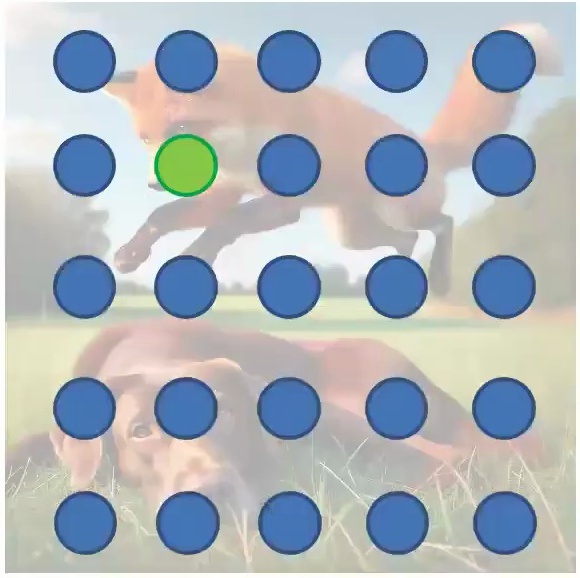
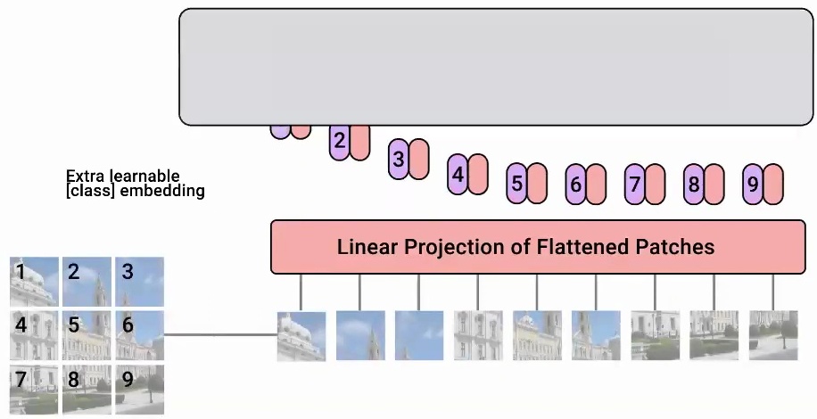
Vision Transformers apply the same fundamental principles that make convolutional neural networks effective for spatial data – they need to be invariant to spatial translation. What Vision Transformers do is cut the original image into patches, treating each \(K \times K\) patch as a separate component. So instead of processing the entire image at once, they divide it into distinct parts and treat these as a sequence, just like how you would treat a sequence of words in natural language processing.

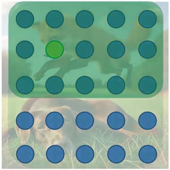
The transformer then learns features for every patch by computing attention scores with respect to each of the other patches and itself. This attention mechanism allows each patch to aggregate information from all other patches in the image, creating rich contextual representations.

The attention mechanism naturally aggregates information over the \(K \times K\) patch regions through the equation:

$$h = \text{softmax}\left(\frac{XW_q W_k^T X^T}{\sqrt{d}}\right) XW_v$$

💡 Key Insight: Patches as Tokens

The key insight is that Vision Transformers maintain the same beneficial properties as convolutional networks through parameter sharing across each of these \(K \times K\) regions. The same parameters are used across all patches, ensuring translation invariance. Additionally, the attention mechanism naturally aggregates information over the patch regions, making the model robust to small shifts and movements across patches.

You can think of these patches as similar to the receptive fields in convolutional layers, but implemented through the attention mechanism instead. This approach has proven remarkably effective, as demonstrated in the seminal work by Dosovitskiy et al. “An image is worth 16×16 words: Transformers for image recognition at scale” (ICLR 2021) that showed transformers can achieve state-of-the-art performance on image recognition tasks.

🔴 From Grids to Graphs

Now, having seen how transformers handle the structured grid of image patches, let’s explore how they can be adapted for an even more complex data structure: graphs.

Finally, we come to graphs, which represent yet another fascinating form of data structure. Graphs consist of nodes that are interconnected in various ways, creating complex relational patterns that differ significantly from the sequential or grid-like structures we’ve seen in other data types. This nodal structure presents unique challenges and opportunities when we consider applying transformer-like architectures to graph-based data.

Molecular Structures and Node Connections

The key insight is that you want to share parameters across each node because without this sharing, the model wouldn’t be able to generalize to new nodes or entirely new graphs. This concept of information aggregation focuses on examining what features exist in your neighbors and extracting those features from them.

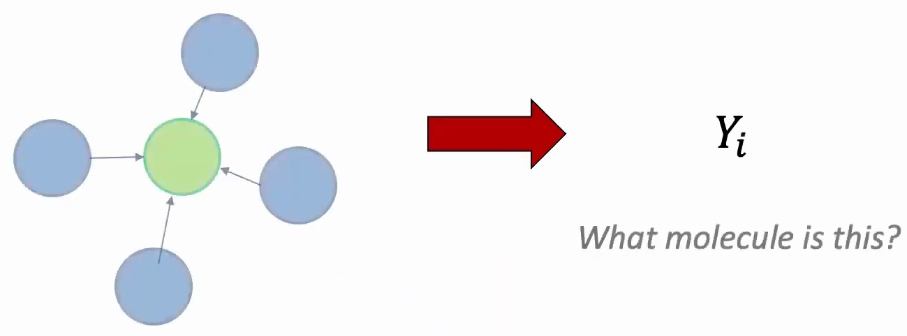
Let’s consider a concrete example: suppose you want to learn a feature representation for node A, where A represents a person in your social network. To accomplish this, you first examine A’s neighbors – perhaps nodes B and C, which represent A’s friends in the social network. However, learning features for C requires looking at C’s connections to A and B, while B depends on its connections to friends A and E, and E in turn depends on its relationships with A and B.

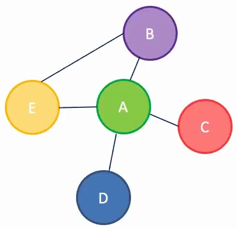
This creates a recursive dependency structure where each node’s representation depends on its neighbors’ features. The model design follows a neural network architecture where you learn features by taking the embeddings of neighboring nodes, passing them through nonlinear transformations, and recursively applying this process to the neighbors of neighbors. All nodes execute the same function, maintaining parameter sharing, while aggregating information based on the connectivity patterns between nodes.

💡 Graphs as a Unifying Framework

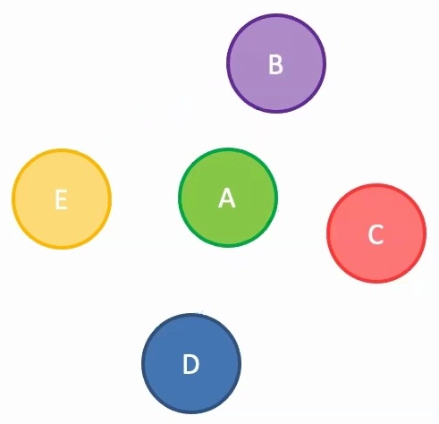
What’s particularly fascinating is that graphs can recover simpler data structures as special cases:

Sets as Graphs: Sets are essentially graphs containing only nodes with no edges connecting them – the same parameter sharing logic applies, but there’s no aggregation step since nodes have no neighbors.

Spatial Data as Graphs: Images can be viewed as graphs where pixels are connected to neighbors within some local region, creating structured connectivity patterns that graph networks can naturally handle.

Graph Recovery and Spatial-Temporal Data

Building on our understanding of graph structures, we can now see how they provide a unified framework for analyzing various deep learning architectures and their data processing patterns. When working with spatial data, you might connect regions based on their proximity – for instance, connecting region two to region three because they represent areas where the image should be spatially linked.

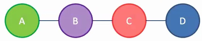
This concept extends naturally to different data types, where sequences can be viewed as graphs arranged in a simple chain structure. A key insight is that sequences are essentially graphs organized in a chain formation, which explains why many models we’ve encountered share common architectural principles.

Parameter sharing across nodes extends naturally to set elements, where the same model processes elements A, B, C, and D uniformly. Information aggregation consistently occurs across neighbors – for sequential data, this means aggregating information from left and right neighbors, while for spatial data, information flows up, down, left, and right among neighboring elements.

Unified View: All Architectures Through Graphs

This unified framework enables you to understand and design your own deep learning architectures by recognizing these fundamental patterns. Whether you’re working with sequences, images, sets, or complex graph structures, the same principles of parameter sharing and neighbor-based information aggregation apply – just with different connectivity patterns defining who the “neighbors” are for each data type.

The Modeling Decision Framework

When approaching any AI problem, one of the biggest decisions you’ll need to make is choosing your modeling paradigm. You have to decide whether to adapt and fine-tune an existing general-purpose model, or build a domain-specific model tailored to your particular setting. Throughout this guide, we’ve looked at more domain-specific methods for each modality and how to build custom architectures for settings like graphs.

The modeling process starts with crucial data decisions:

• Decide how much data to collect and how much to label, considering both costs and time constraints
• Clean your data by normalizing and standardizing it, finding noisy data points, and performing anomaly or outlier detection
• Visualize your data through plotting, dimensionality reduction techniques like PCA or t-SNE, and cluster analysis

💡 The Core Modeling Challenge

Once your data is prepared, you need to establish your evaluation framework and break down the complexity of your data:

• Decide on evaluation metrics that include both proxy and real metrics, as well as quantitative and qualitative measures
• Figure out how to break down complex data into individual elements – whether these elements are organized sequentially, spatially, or as elements of a set or graph
• Determine the base elements and how to represent them effectively

A critical aspect of model design is understanding data invariances and equivariances: Invariances are properties that the model should not be sensitive to, while equivariances are what the model should be sensitive to. If you’re not careful about identifying these properties, you can blow up the number of samples your model will need to train effectively.

🔴 The Iterative Nature of Model Development

The entire process is iterative. You’ll typically cycle between data collection, model design, model training, hyperparameter tuning, and evaluation until you’re satisfied with the results. This iterative approach allows you to refine each component based on what you learn from the others.

Unifying Architecture Paradigms

While we’ve examined domain-specific methods for different modalities, there are underlying principles that connect these seemingly disparate approaches:

The common thread running through all these architectural paradigms is the fundamental challenge of representation learning – how we transform raw data into meaningful representations that capture the essential structure and relationships within our problem domain.

Whether we’re dealing with sequential data, spatial information, or graph structures, the core principles of attention, hierarchical feature extraction, and adaptive computation remain consistent across different architectural choices:

• Parameter Sharing: Reusing the same learned transformations across different parts of the input
• Information Aggregation: Combining local features into increasingly global representations
• Hierarchical Processing: Building from simple to complex features through multiple layers
• Invariance and Equivariance: Respecting the fundamental symmetries in the data

Final Key Takeaways

• Universal Framework: All deep learning architectures can be understood through the lens of learning representations and combining them hierarchically, with specific designs emerging from the structure and invariances in your data.
• Architecture as Prior Knowledge: Careful architectural choices that respect data symmetries (like translation invariance for images or permutation invariance for sets) can dramatically reduce the amount of training data required.
• From Domain-Specific to General: The spectrum from highly specialized custom architectures to general-purpose models like transformers represents different trade-offs between sample efficiency and flexibility.
• Graphs as Unifying Abstraction: Viewing different data types through the graph lens – sequences as chains, images as grids, sets as disconnected nodes – provides a powerful unified framework for understanding all architectures.
• Attention Revolutionized Everything: The attention mechanism, born from sequence-to-sequence translation, has become the foundation of modern architectures across all modalities, enabling parallel processing and long-range dependencies.
• Iterative Refinement: Model development is fundamentally iterative – cycling between data preparation, architecture design, training, and evaluation until achieving satisfactory results.

Moving Forward

This unified perspective on architecture design provides you with a solid foundation for approaching any deep learning problem. Understanding these common principles will serve you well as you tackle new challenges and begin to design your own architectures.

Remember that successful modeling depends on understanding your data’s structure, identifying the right invariances and equivariances, choosing appropriate representations, and iteratively refining your approach based on empirical results. Whether you’re working with text, images, graphs, or any other data modality, these fundamental principles remain constant.

The field of deep learning continues to evolve rapidly, with new architectures and techniques emerging regularly. However, by grounding yourself in these fundamental principles – parameter sharing, hierarchical representation learning, attention mechanisms, and respect for data structure – you’ll be well-equipped to understand, evaluate, and contribute to these advances.