LLM_log #001: Understanding Large Language Models: From Word Counting to Neural Networks
Part 1: The Evolution of Text Representation
🚀 The AI Revolution: How We Got Here
The period from 2012 to today marked a fundamental transformation in artificial intelligence. Deep neural networks enabled systems that can understand and generate human language with unprecedented accuracy.
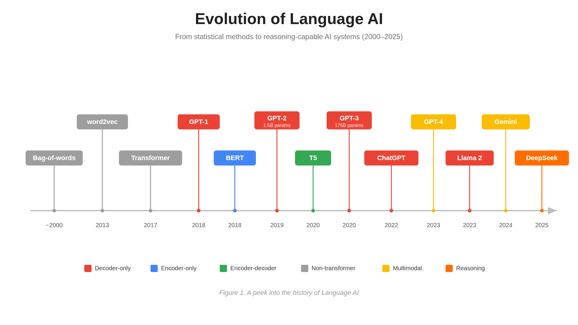 Figure 0: From word embeddings to reasoning-capable AI systems – the complete LLM timeline
The ChatGPT Moment
November 2022 brought ChatGPT – an application that:
- Reached 1 million users in 5 days
- Surpassed 100 million users in 2 months
- Became the fastest-growing consumer application in history
This wasn’t just another AI product – it was proof that language models were ready to transform how we interact with technology.
Where Are We Now? (2025-2026)
The field has accelerated dramatically:
- DeepSeek-R1 brought open reasoning models with RLVR training
- GPT-5 introduced 400K context windows and improved reasoning
- Claude 4.5 excels at computer use with 200K context
- Llama 4 adopted Mixture-of-Experts architecture
- RLVR Era – Reinforcement Learning from Verifiable Rewards is reshaping training
💡 What Is Language AI?
Language AI encompasses computational systems designed to:
- Understand human language in context
- Process textual information at scale
- Generate coherent, contextually appropriate responses
This field combines classical Natural Language Processing (NLP) with modern machine learning techniques.
Why Is Language Hard for Computers?
Text is fundamentally unstructured. Unlike tabular data or images with fixed dimensions:
- Variable length: Sentences and documents vary dramatically in size
- Context-dependent: The same word can have different meanings
- Ambiguous: Natural language contains inherent ambiguity
Computers process binary information (0s and 1s). Transforming unstructured text into meaningful numerical representations has been the central challenge of Language AI.
📊 Evolution of Text Representation
Let’s trace the historical evolution of how computers “see” text – from the simplest methods to sophisticated neural approaches.
PHASE 1: Bag-of-Words (2000s)
Core Idea: Represent text by counting word occurrences, ignore order and grammar.
How Does It Work?
The process happens in three steps:
Step 1: Tokenization – Split text into individual words
"Machine learning is powerful" → ["Machine", "learning", "is", "powerful"]Step 2: Vocabulary Creation – Collect all unique words
Vocabulary: ["Machine", "learning", "is", "powerful", "AI", "models"]Step 3: Word Counting – Create numerical vectors based on frequency
"Machine learning is powerful" → [1, 1, 1, 1, 0, 0]
"AI models are powerful"       → [0, 0, 0, 1, 1, 1]
Practical Example
Let’s analyze two simple statements:
Statement 1: “This is a sweet cat”
Statement 2: “My cat is sweet”
Step 1: Tokenization
First, we break each sentence into individual word tokens:
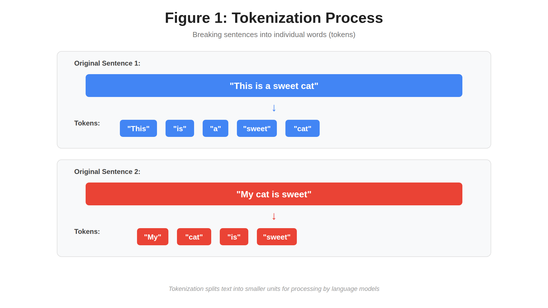
Figure 1: Breaking sentences into individual words (tokens)
Step 2: Vocabulary Creation
Next, we merge all unique words from both sentences to create a unified vocabulary:
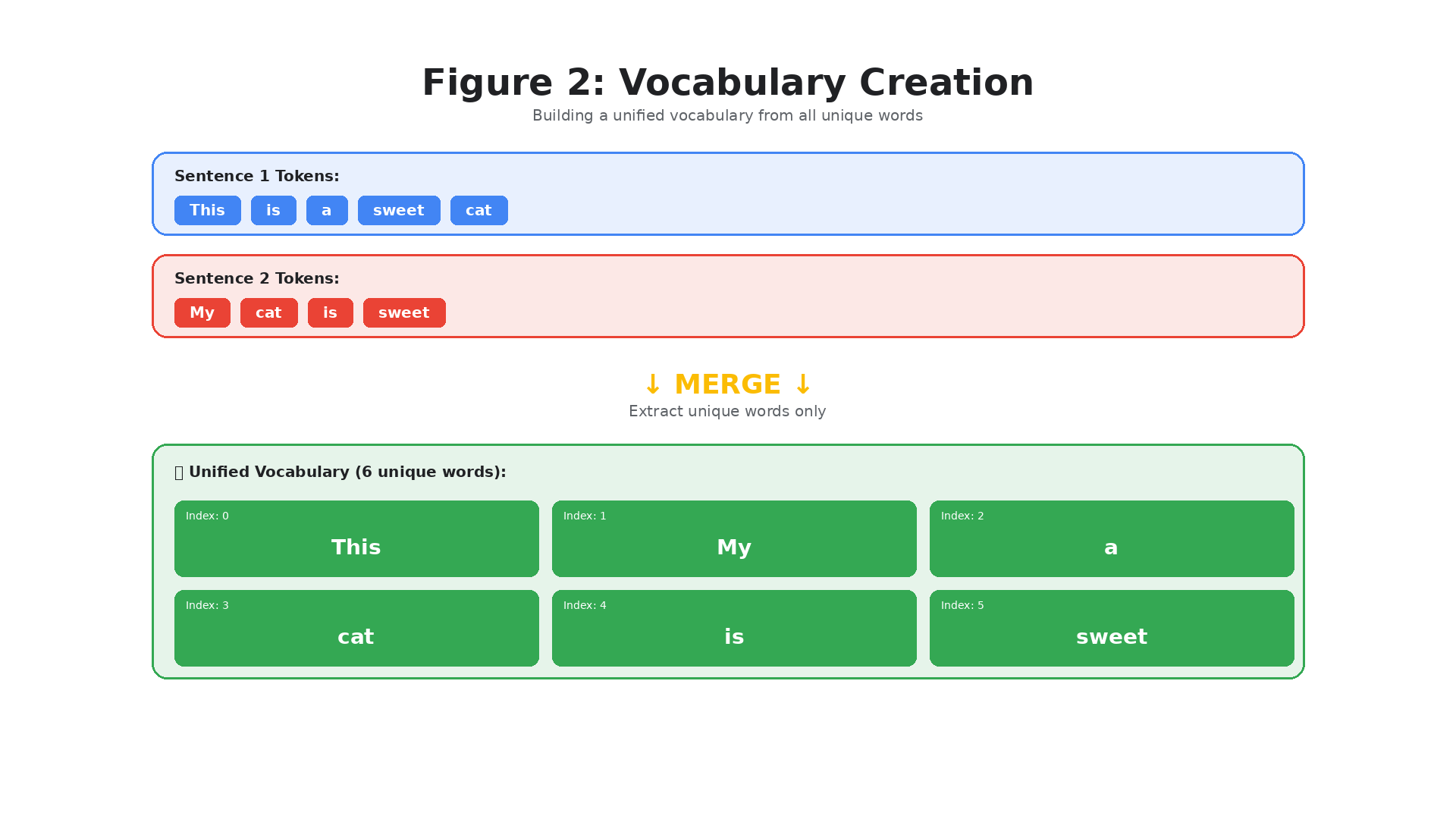
Figure 2: Building a unified vocabulary from all unique words (6 total)
Step 3: Bag-of-Words Vectors
Finally, we count occurrences of each vocabulary word in each sentence:

Figure 3: Converting text into numerical vectors by counting word occurrences
Notice how:
- Sentence 1 “This is a sweet cat” →
[1, 0, 1, 1, 1, 1] - Sentence 2 “My cat is sweet” →
[0, 1, 0, 1, 1, 1]
Both sentences share “cat”, “is”, and “sweet” (the last three positions), but differ in “This”, “My”, and “a”.
Advantages and Limitations
✅ Advantages:
- Simple to implement
- Computationally efficient
- Good for basic tasks (spam detection, basic classification)
- Still useful in certain scenarios
❌ Limitations:
- Ignores word order: “dog bites man” = “man bites dog”
- No semantic understanding: Can’t distinguish similar meanings
- High dimensionality: Large vocabularies create huge vectors
- No context: “bank” (financial) vs “bank” (river) – same representation
PHASE 2: Dense Embeddings – word2vec (2013)
The Breakthrough: Represent words as dense vectors that capture semantic meaning.
Core Principle: “You shall know a word by the company it keeps”
Words appearing in similar contexts have similar meanings. This simple idea revolutionized NLP.
How word2vec Works
Step 1: Initialize random vectors for each word (e.g., 300 dimensions)
Step 2: Create training pairs from text
"The cat sat on the mat"
     ↓
Target: "sat"
Context: ["cat", "on"]
Step 3: Train neural network to predict if words appear together
Step 4: Extract learned embeddings as word representations
Magic of Embeddings
The resulting vectors have amazing properties:
- Semantic similarity → geometric proximity
- Mathematical operations capture relationships:
king - man + woman ≈ queenParis - France + Italy ≈ Rome
- Word clusters form naturally:
- “happy”, “joyful”, “pleased” → nearby vectors
- “sad”, “unhappy”, “depressed” → different cluster

Figure 4: 2D projection showing how semantically similar words cluster together. Animals (blue), positive emotions (green), negative emotions (red), and food (yellow) each form distinct regions.
This visualization demonstrates the core insight: meaning becomes geometry. Words with similar meanings end up close together in the embedding space.
The Limitation of word2vec: Static Representations
The training process of word2vec creates static, downloadable representations of words. Once trained, the embedding for a word never changes. For instance, the word “spring” will always have the same embedding regardless of the context in which it is used.
However, “spring” can refer to:
- A season: “I love spring when flowers bloom”
- A coiled metal device: “The spring in my mattress broke”
- A water source: “We found a natural spring in the mountains”
- An action: “Watch the cat spring onto the table”
Its meaning, and therefore its embedding, should change depending on the context. But with word2vec, all four meanings get compressed into a single vector — a fundamental limitation.
PHASE 3: Contextual Representations with RNNs
A step toward encoding contextual information was achieved through Recurrent Neural Networks (RNNs). These are variants of neural networks that can model sequences by treating previous outputs as additional inputs.
What Makes RNNs “Autoregressive”?
RNNs are autoregressive models. This means the current output depends on previous outputs. Each step in the sequence uses information from all preceding steps.
Side note — Autoregressive in equations:
A simple autoregressive process might look like:
\(\varepsilon_t = \varepsilon_{t-1} + 3 \cdot \varepsilon_{t-2}\)
Here, each value depends on the two values that came before it.
Practical intuition: Imagine predicting the next word in a sentence. If you’ve generated “The cat sat on the…”, your prediction for the next word depends heavily on what you’ve already said. You’re more likely to predict “mat” or “floor” than “airplane” — because you’re conditioning on the previous context. That’s autoregressive prediction in action.
The Encoder-Decoder Architecture
RNNs are used for two complementary tasks:
- Encoding: Representing (compressing) an input sentence into a fixed-size vector
- Decoding: Generating an output sentence from that representation
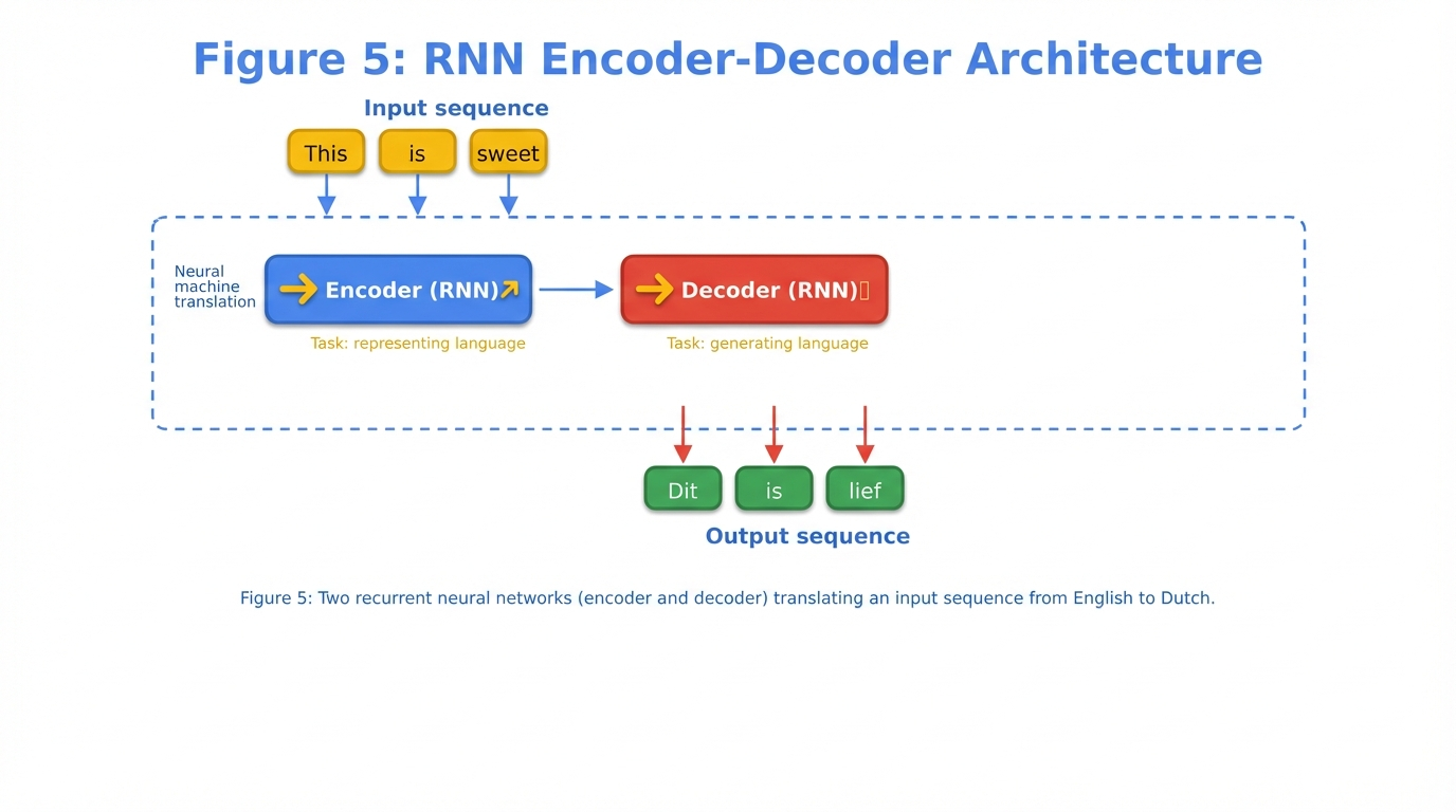
Figure 5: Two recurrent neural networks (encoder and decoder) translating an input sequence from English to Dutch.
The encoder reads the input sequence “This is sweet” and compresses it into a context embedding. The decoder then uses this embedding to generate the Dutch translation “Dit is lief” one word at a time.
Autoregressive Generation Step-by-Step
Because the architecture is autoregressive, when generating the next word, the decoder must consume all previously generated words:
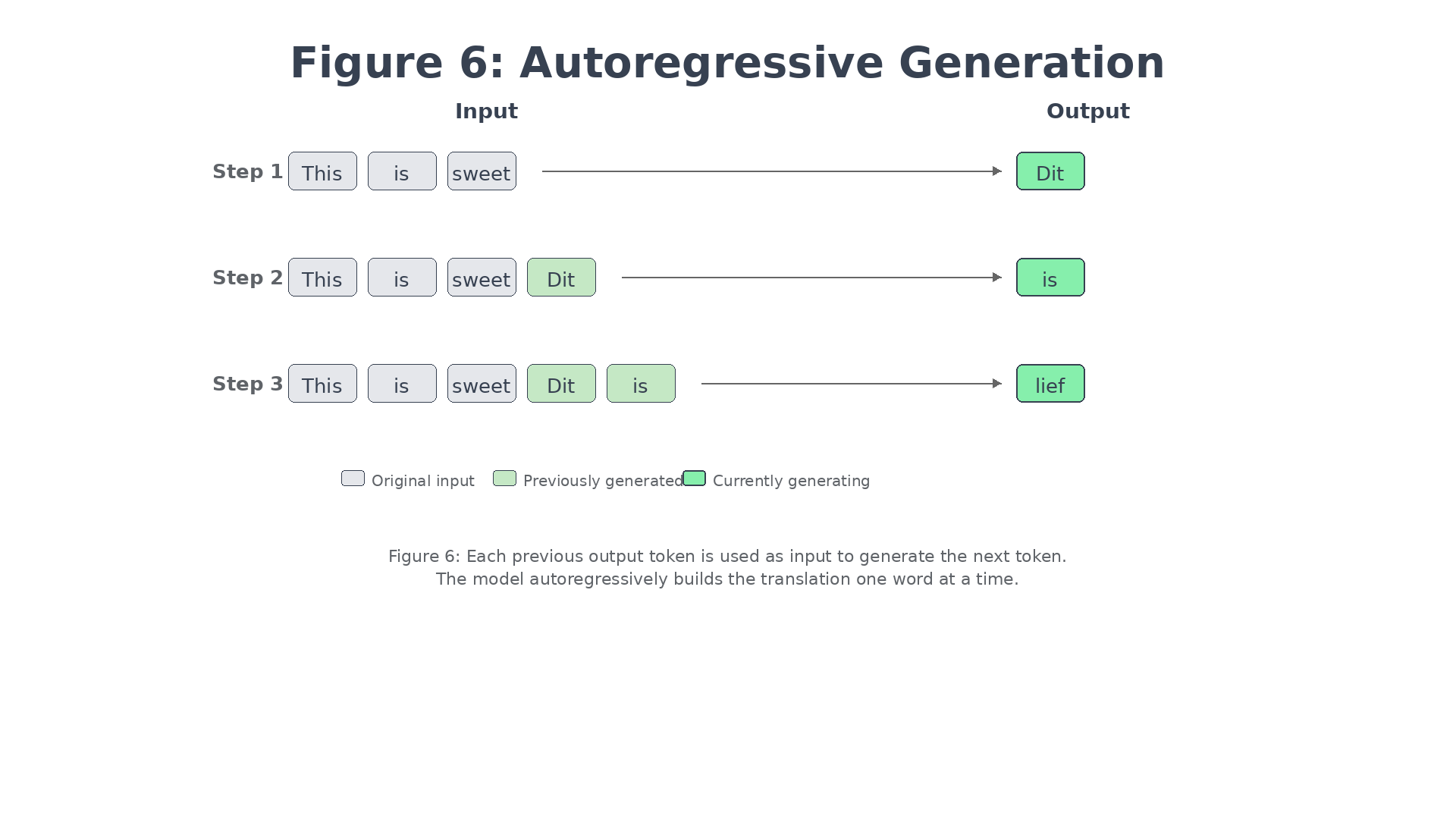
Figure 6: Each previous output token is used as input to generate the next token. The model builds the translation one word at a time.
At each step:
- Step 1: Input is “This is sweet” → Output: “Dit”
- Step 2: Input is “This is sweet” + “Dit” → Output: “is”
- Step 3: Input is “This is sweet” + “Dit is” → Output: “lief”
Why This Approach Had Limitations
The encoder compresses the entire input sequence into a single fixed-size context embedding. This creates a bottleneck — for longer sentences, critical information gets lost in the compression. The decoder has no way to “look back” at specific parts of the input; it only sees the compressed summary.
This limitation becomes severe with longer sequences, where important details from the beginning of the input may be forgotten by the time they’re needed for generation.
The Introduction of Attention (2014)
In 2014, a solution called attention was introduced that dramatically improved upon the original RNN architecture.
The core insight: instead of forcing all information through a single bottleneck embedding, why not let the decoder look directly at the input sequence and focus on the most relevant parts for each output word?
Attention allows the model to selectively focus on parts of the input sequence that are relevant to the current output being generated. Different input words get different “attention weights” depending on how useful they are for predicting the current output.
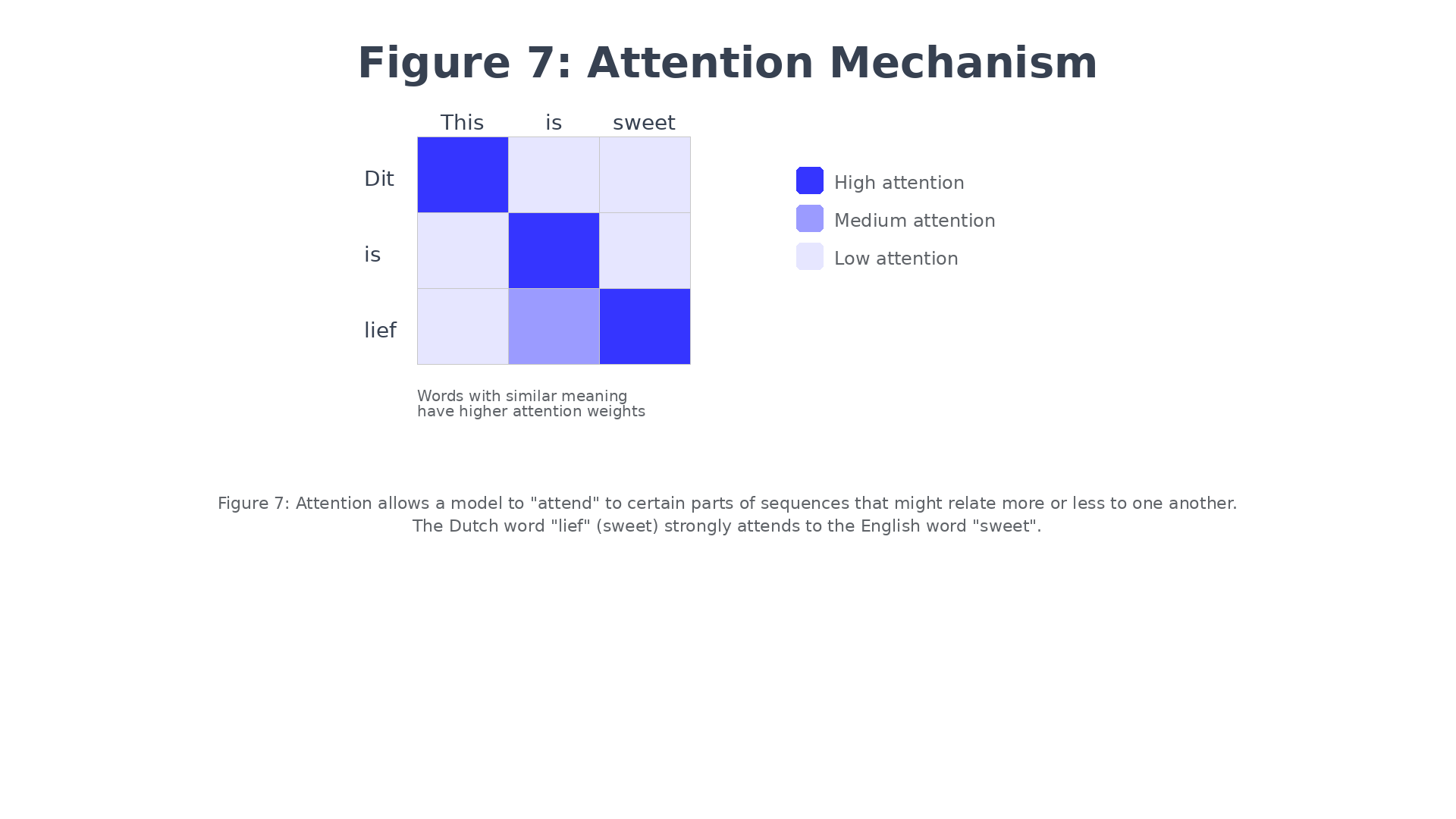
Figure 7: Attention allows a model to “attend” to certain parts of sequences that might relate more or less to one another.
When generating “lief” (the Dutch word for “sweet”), the attention mechanism assigns a high weight to the English word “sweet” because they share meaning. Meanwhile, “Dit” attends strongly to “This”, and “is” attends to “is”. The model learns these alignments automatically during training.
🔄 The Transformer: “Attention Is All You Need”
The true power of attention, and what drives the capabilities of modern large language models, was first explored in the landmark paper “Attention is all you need” released in 2017.
The authors proposed a network architecture called the Transformer, which was based solely on the attention mechanism — completely removing the recurrent connections that we saw in RNNs.
This was revolutionary for one key reason: unlike RNNs that must process sequences one step at a time, Transformers can process all positions in parallel. This dramatically sped up training and enabled scaling to much larger models.
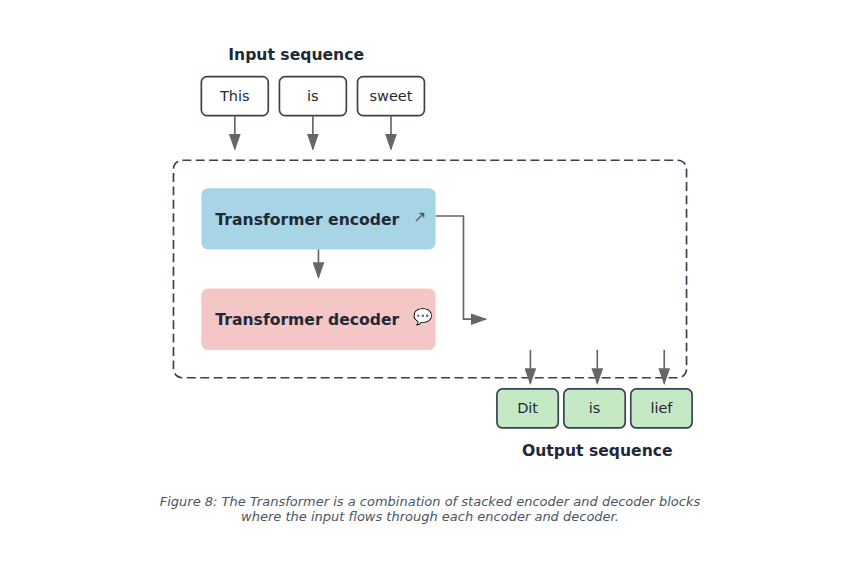
Figure 8: The Transformer is a combination of stacked encoder and decoder blocks where the input flows through each encoder and decoder.
The Transformer retains the encoder-decoder structure, but both components now use attention mechanisms instead of recurrence.
The Transformer Encoder
The encoder block in the Transformer consists of two main parts:
- Self-attention layer
- Feedforward neural network
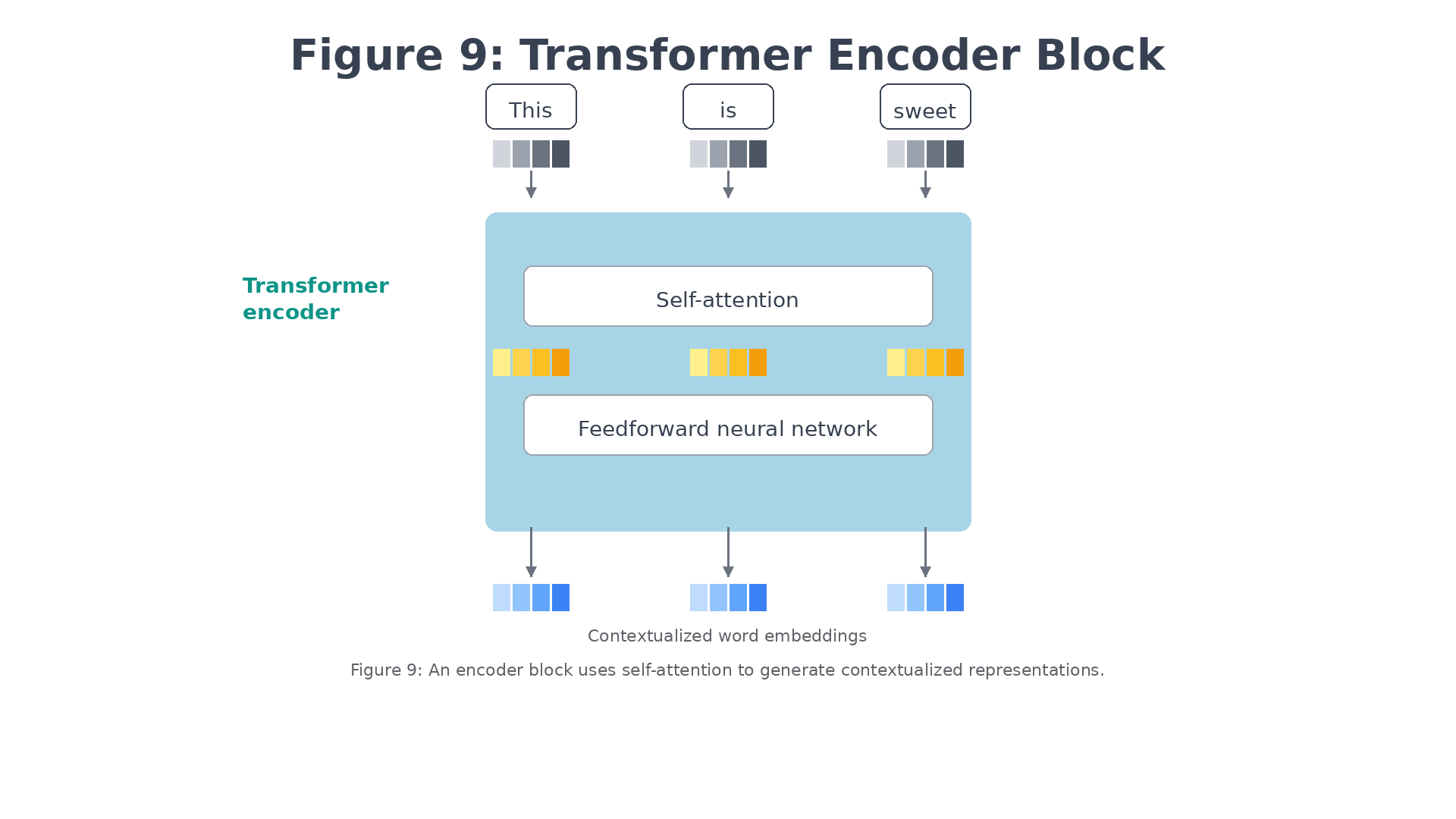
Figure 9: An encoder block revolves around self-attention to generate intermediate representations.
What is Self-Attention?
Unlike the attention mechanism in RNNs (which attended from decoder to encoder), self-attention allows each position in a sequence to attend to all other positions in the same sequence.
When processing the word “sweet” in “This is sweet”, self-attention can look at both “This” and “is” simultaneously to understand the full context. It can “look” both forward and backward in the sequence in a single operation.
This is powerful because:
- The word “This” can gather information from “is” and “sweet”
- The word “is” can gather information from “This” and “sweet”
- The word “sweet” can gather information from “This” and “is”
All of this happens in parallel, producing contextualized embeddings where each word’s representation is informed by the entire sequence.
The Transformer Decoder
The decoder has a similar structure to the encoder, but with an important addition: an extra attention layer that attends to the encoder’s output.
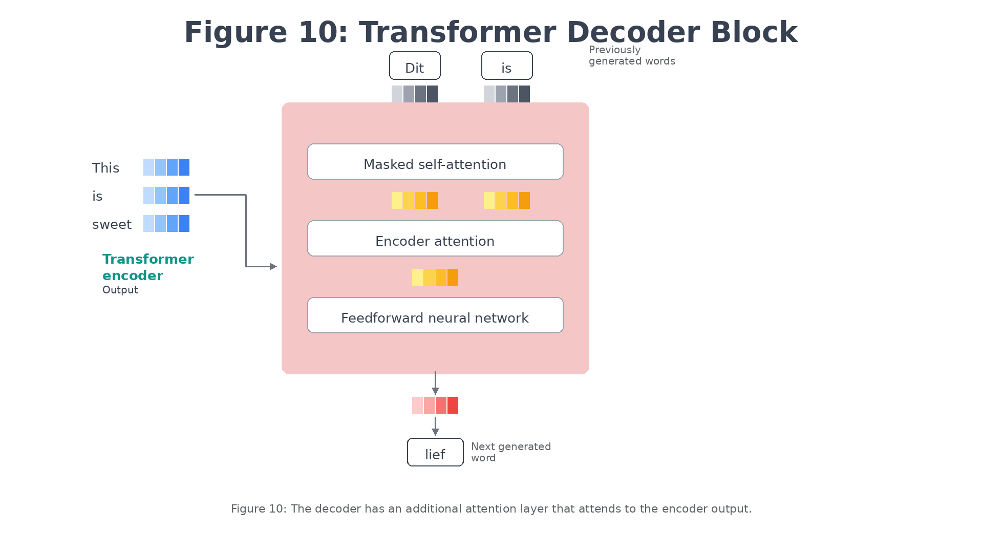
Figure 10: The decoder has an additional attention layer that attends to the encoder’s output.
The decoder consists of three layers:
- Masked self-attention: Attends to previously generated output tokens
- Encoder attention: Attends to the encoder’s output (to find relevant parts of the input)
- Feedforward neural network: Processes the combined information
After generating “Dit” and “is”, the encoder attention layer enables the decoder to focus on the relevant input word “sweet” before generating the Dutch translation “lief”.
Masked Self-Attention: Preventing “Cheating”
There’s a critical constraint in the decoder’s self-attention: it can only attend to earlier positions, not future ones. This is called masked self-attention.
Why is this necessary? During training, we show the decoder the complete target sequence. But during generation, future words don’t exist yet — we’re creating them one at a time. If the decoder could see future tokens during training, it would learn to “cheat” by just copying them, and fail completely during actual generation.
The mask ensures that when predicting position t, the model can only use information from positions 1 through t-1. This makes training consistent with generation.
🎯 Key Takeaways
- Text representation evolved from simple counting to sophisticated neural embeddings
- Bag-of-Words was simple but lost word order and semantics
- word2vec captured semantic relationships but created static representations
- RNNs introduced sequential processing and context, but suffered from bottleneck issues
- Attention allowed models to focus on relevant parts of the input
- Transformers combined self-attention and encoder-decoder architecture, enabling parallel processing and modern LLMs
📚 Modern Language Model Architectures
Representation Models: Encoder-Only Models
The original Transformer model is an encoder-decoder architecture that serves translation tasks well but cannot easily be used for other tasks, like text classification.
In 2018, a new architecture called Bidirectional Encoder Representations from Transformers (BERT) was introduced that could be leveraged for a wide variety of tasks and would serve as the foundation of Language AI for years to come. BERT is an encoder-only architecture that focuses on representing language, as illustrated in Figure 11. This means that it only uses the encoder and removes the decoder entirely.
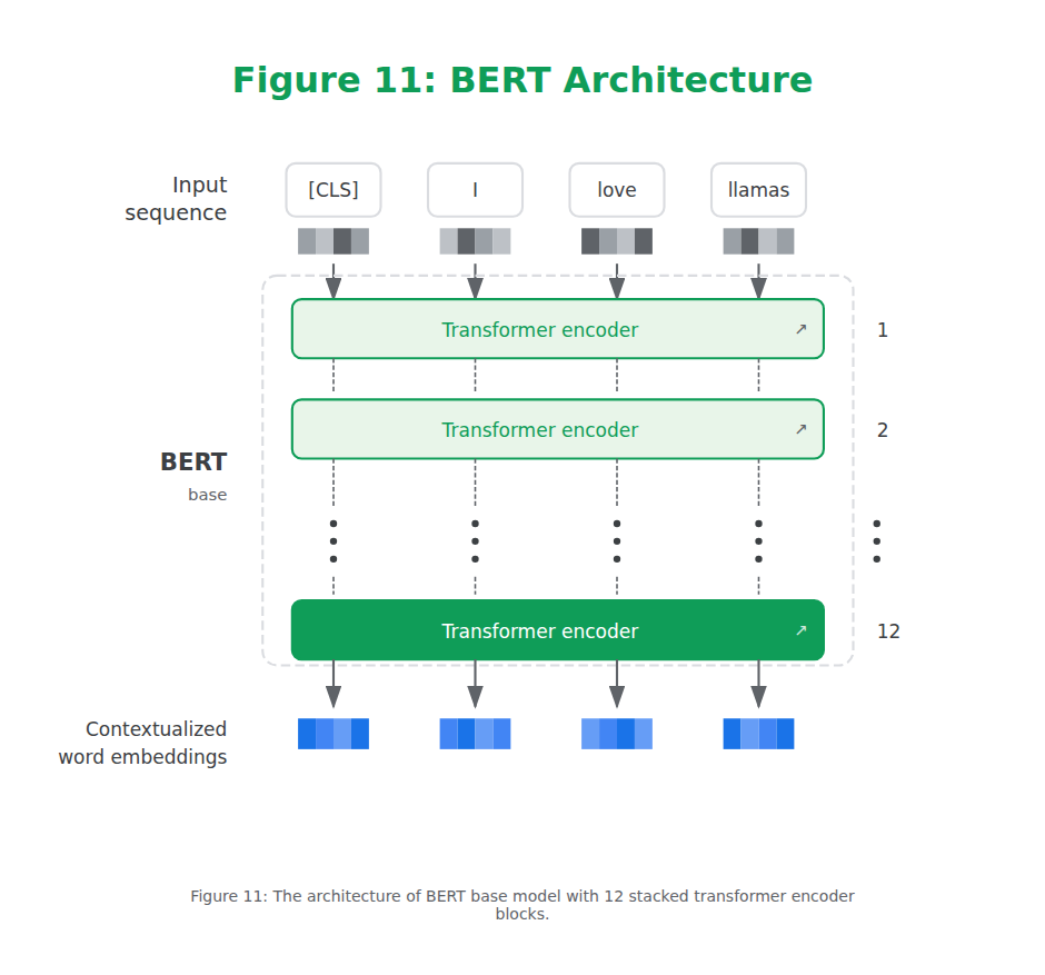
Figure 11: The architecture of BERT base model with 12 stacked transformer encoder blocks.
These encoder blocks are the same as we saw before: self-attention followed by feedforward neural networks. The input contains an additional token, the [CLS] or classification token, which is used as the representation for the entire input. Often, we use this [CLS] token as the input embedding for fine-tuning the model on specific tasks, like classification.
Training these encoder stacks can be a difficult task that BERT approaches by adopting a technique called masked language modeling. This method masks a part of the input for the model to predict. This prediction task is difficult but allows BERT to create more accurate (intermediate) representations of the input.
This architecture and training procedure makes BERT and related architectures incredible at representing contextual language. BERT-like models are commonly used for transfer learning, which involves first pretraining it for language modeling and then fine-tuning it for a specific task. For instance, by training BERT on the entirety of Wikipedia, it learns to understand the semantic and contextual nature of text. Then, we can use that pretrained model to fine-tune it for a specific task, like text classification.
A huge benefit of pretrained models is that most of the training is already done for us. Fine-tuning on specific tasks is generally less compute-intensive and requires less data. Moreover, BERT-like models generate embeddings at almost every step in their architecture. This also makes BERT models feature extraction machines without the need to fine-tune them on a specific task.
Encoder-only models, like BERT, will be used in many parts of the book. For years, they have been and are still used for common tasks, including classification tasks, clustering tasks, and semantic search.
Throughout the book, we will refer to encoder-only models as representation models to differentiate them from decoder-only, which we refer to as generative models. Note that the main distinction does not lie between the underlying architecture and the way these models work. Representation models mainly focus on representing language, for instance, by creating embeddings, and typically do not generate text. In contrast, generative models focus primarily on generating text and typically are not trained to generate embeddings.
Generative Models: Decoder-Only Models
Similar to the encoder-only architecture of BERT, a decoder-only architecture was proposed in 2018 to target generative tasks. This architecture was called a Generative Pre-trained Transformer (GPT) for its generative capabilities (it’s now known as GPT-1 to distinguish it from later versions). As shown in Figure 12, it stacks decoder blocks similar to the encoder-stacked architecture of BERT.
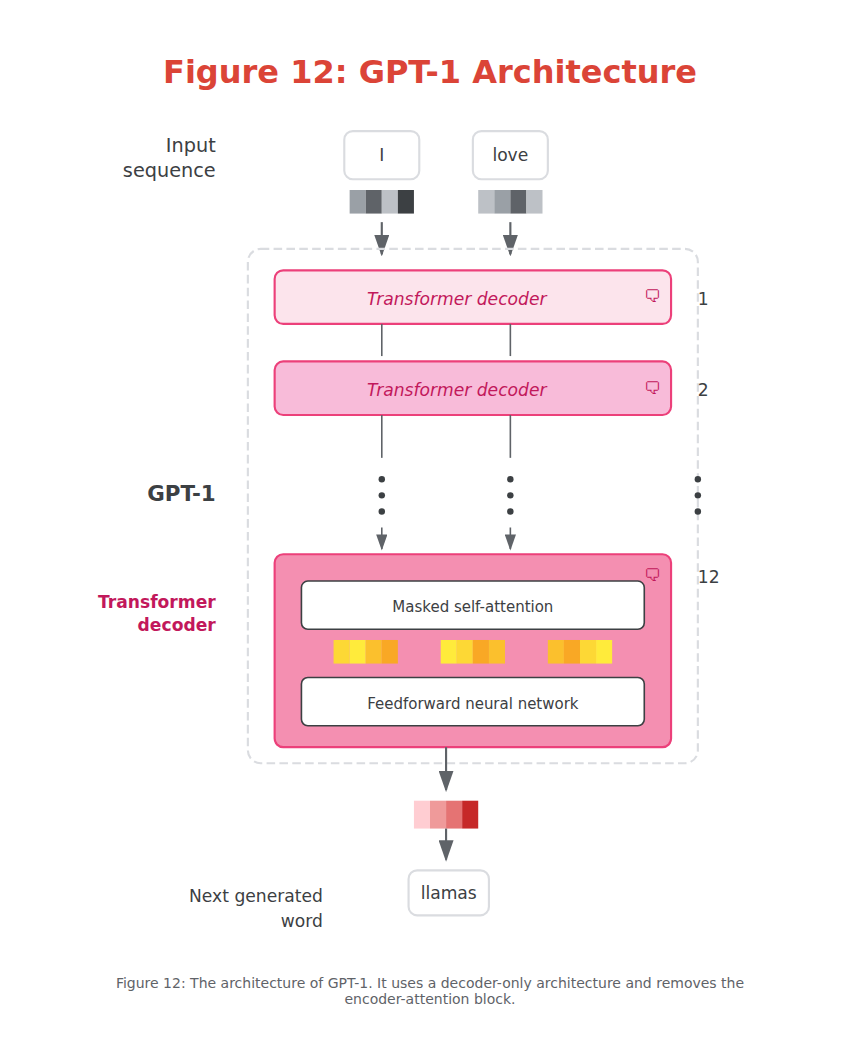
Figure 12: The architecture of GPT-1. It uses a decoder-only architecture and removes the encoder-attention block.
GPT-1 was trained on a corpus of 7,000 books and Common Crawl, a large dataset of web pages. The resulting model consisted of 117 million parameters. Each parameter is a numerical value that represents the model’s understanding of language.
If everything remains the same, we expect more parameters to greatly influence the capabilities and performance of language models. Keeping this in mind, we saw larger and larger models being released at a steady pace. GPT-2 had 1.5 billion parameters and GPT-3 used 175 billion parameters quickly followed.
These generative decoder-only models, especially the “larger” models, are commonly referred to as large language models (LLMs). As we will discuss later in this chapter, the term LLM is not only reserved for generative models (decoder-only) but also representation models (encoder-only).
Generative LLMs, as sequence-to-sequence machines, take in some text and attempt to autocomplete it. Although a handy feature, their true power shone from being trained as a chatbot. Instead of completing a text, what if they could be trained to answer questions? By fine-tuning these models, we can create instruct or chat models that can follow directions.

Figure 13: Generative LLMs take in some input and try to complete it. With instruct models, this is more than just autocomplete and attempts to answer the question.
As illustrated in Figure 13, the resulting model could take in a user query (prompt) and output a response that would most likely follow that prompt. As such, you will often hear that generative models are completion models.
Context Length
A vital part of these completion models is something called the context length or context window. The context length represents the maximum number of tokens the model can process, as shown in Figure 14. A large context window allows entire documents to be passed to the LLM. Note that due to the autoregressive nature of these models, the current context length will increase as new tokens are generated.
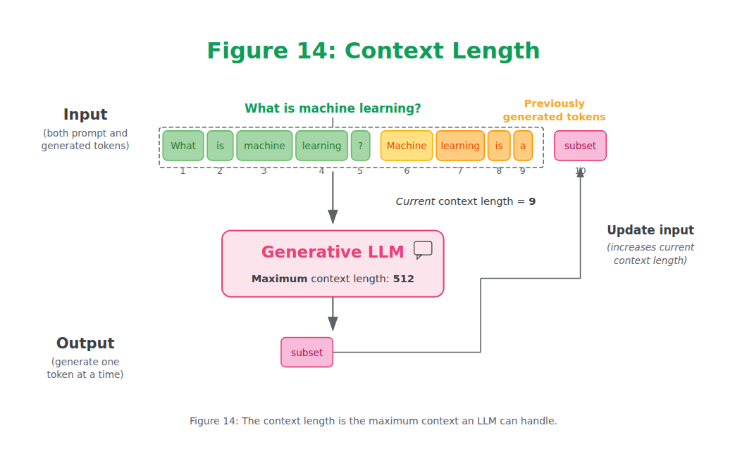
Figure 14: The context length is the maximum context an LLM can handle.
🔧 The Training Paradigm of Large Language Models
Traditional machine learning generally involves training a model for a specific task, like classification. We consider this to be a one-step process.
Creating LLMs, in contrast, typically consists of at least two steps:
Language modeling
The first step, called pretraining, takes the majority of computation and training time. An LLM is trained on a vast corpus of internet text allowing the model to learn grammar, context, and language patterns. This broad training phase is not yet directed toward specific tasks or applications beyond predicting the next word. The resulting model is often referred to as a foundation model or base model. These models generally do not follow instructions.
Fine-tuning
The second step, fine-tuning or sometimes post-training, involves using the previously trained model and further training it on a narrower task. This allows the LLM to adapt to specific tasks or to exhibit desired behavior. For example, we could fine-tune a base model to perform well on a classification task or to follow instructions. It saves massive amounts of resources because the pretraining phase is quite costly and generally requires data and computing resources that are out of the reach of most people and organizations. For instance, Llama 2 has been trained on a dataset containing 2 trillion tokens. Imagine the compute necessary to create that model!
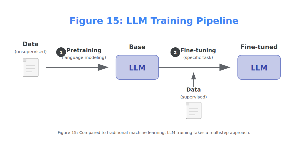
Figure 15: Compared to traditional machine learning, LLM training takes a multistep approach.
Any model that goes through the first step, pretraining, we consider a pretrained model, which also includes fine-tuned models. This two-step approach of training is visualized in Figure 15.
Additional fine-tuning steps can be added to further align the model with the user’s preferences.