#012A Building a Deep Neural Network
Building blocks of a Deep Neural Network
In this post we will see what are the building blocks of a Deep Neural Network.
We will pick one layer, for example layer \(l \) of a deep neural network and we will focus on computatons for that layer. For layer \(l \) we have parameters \(\textbf{W}^{[l]} \) and \( b^{[l]} \). Calculation of the forward pass for layer \( l \) we get as we input activations from the previous layer and as the output we get activations of the current layer, layer \(l \).
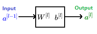
Diagram of a Forward pass through layer \(l \)
Equations for this calculation step are :
\(z^{[l]} = \textbf{W}^{[l]}\color {Blue}{a^{[l-1]}} + b^{[l]} \)
\(\color {Green} {a^{[l]}} = g(z^{[l]}) \)
where \(g(z^{[l]}) \) is an activation function in the layer \(l \).
It is good to cache the value of \( z^{[l]} \) for calculations in backwardpass.
Backward pass is done as we input \(da^{[l]} \) and we get the output \(da^{[l-1]} \), as presented in the following graph. We will always draw backward passes in red.
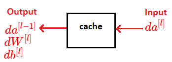
Diagram of a Backward pass through layer \(l \)
In the following picture we can see a diagram of both a forward and a backward pass in the layer \(l \). So, to calulate values in the backward pass we need cached values. Here we just draw \(z^{[l]} \) as a cached value, but indeed we will need to cache also \(W^{[l]} \) and \(b^{[l]} \).
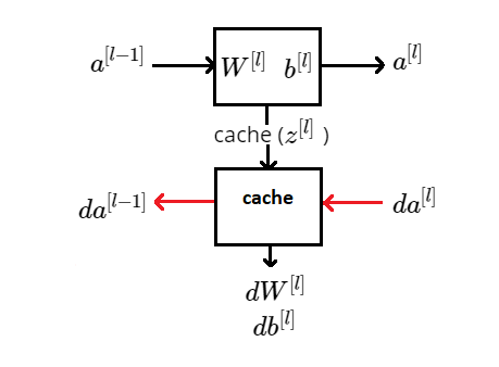
Diagram of a Forward and Backward pass through layer \(l \)
If we implement these two calculations as presented in a graph above, the computation for an \(L \) layer neural network will be as follows. We will get \(a^{[0]} \), which is our feature vector, feed it in, and that will compute the activations of the first layer. The same thing we will do with next layers.

Diagram for a Forward and a Backward pass paths for \(L \) layer Neural Network
Having all derivative terms we can update parameters:
\(\textbf{W}^{[l]} := \textbf{W}^{[l]} – \alpha \textbf{dW}^{[l]} \)
\(b^{[l]} := b^{[l]} – \alpha db^{[l]} \)
In our programming implementation of this algorithm, when we cache \( z^{[l]} \) for backpropagation calculations we will cache also \(\textbf{W}^{[l]} \) and \(b^{[l]} \), and \(a^{[l-1]} \) .
So, building blocks of a deep neural network are the forward step and the corresponding backward step. Next, we will see equations for these steps and their implementation in Python.
Forward and Backward propagation step equations
Here, we will see equations for calculating the forward step.
| Non – Vectorized | Vectorized |
|
\(z^{[l]} = \textbf{W}^{[l]}a^{[l-1]} + b^{[l]} \) \(a^{[l]} = g(z^{[l]}) \) |
\(\textbf{Z}^{[l]} = \textbf{W}^{[l]}\textbf{A}^{[l-1]} + b^{[l]} \) \(\textbf{A}^{[l]} = g(\textbf{Z}^{[l]}) \) |
You can always remind how we have defined matrices \(\textbf{Z}^{[l]} \), \(\textbf{A}^{[l]}\) and \(\textbf{W}^{[l]}\) here.
Here we will see equations for caluculating backward step:
| Non – Vectorized | Vectorized |
|
\(dz^{[l]} = da^{[l]} * g’^{[l]}(z^{[l]}) \enspace \enspace (1)\) \( \textbf{dW}^{[l]} = dz^{[l]} a^{[l-1]} \) \(db^{[l]} = dz^{[l]} \) \(da^{[l-1]} = \textbf{dW}^{[l]T} dz^{[l]}\enspace \enspace (2) \) and from equations \((1) \) and \((2)\) we have: \(dz^{[l]} = \textbf{dW}^{[l+1]T}dz^{[l+1] } * g’^{[l]}(z^{[l]}) \) |
\(\textbf{dZ}^{[l]} = \textbf{dA}^{[l]} *g’^{[l]}(\textbf{Z}^{[l]}) \) \( \textbf{dW}^{[l]} = \textbf{dZ}^{[l]} \textbf{A}^{[l-1]T}\) \(db^{[l]} = \frac{1}{m}np.sum(\textbf{dZ}^{[l]}, axis = 1, keepdims = True) \) \( \textbf{dA}^{[l-1]} = \textbf{W}^{[l]T} \textbf{dZ}^{[l]} \) |
Remember that \(* \) represents an element wise multiplication.
A 2-layer neural network is presented in the picture below:
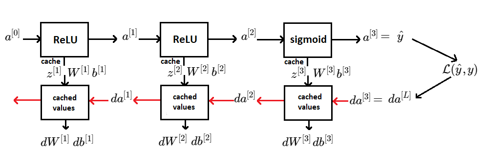
Diagram of a Forward and Backward pass for 2 – layer Neural Network
First, we initialize the forward step of the deep neural network with \(L \) layers, with input feature vector \(x = a^{[0]} \) or with a matrix \(\textbf{X} \) where we stack all training examples horizontally. After computing the final forward step, we get the prediction \(\hat{y}\) and that allows us to compute the loss for that prediction \(\mathcal {L} (\hat{y}, y) \). Within the backward step we initialize with \( da^{[L]} \) and if we are doing binary classification (so sigmoid function is activation in the layer \(L\)) :
\(da^{[L]} = – \frac {y}{a} + \frac {1-y}{1-a} \)
and for vectorized version we have:
\( \textbf{dA}^{[L]} \) = \(\begin {bmatrix} – \frac {y^{(1)}}{a^{(1)}} + \frac {1-y^{(1)}}{1-a^{(1)}} & – \frac {y^{(2)}}{a^{(2)}} + \frac {1-y^{(2)}}{1-a^{(2)}} & \dots & – \frac {y^{(m)}}{a^{(m)}} + \frac {1-y^{(m)}}{1-a^{(m)}} \end {bmatrix} \).
Parameters and Hyperparametes of a Deep Neural Network
For building a deep neural network it is very important to organize both parameters and hyperparameters. Parameters of a deep neural network are \(\textbf{W}^{[1]}, b^{[1]}, \textbf{W}^{[2]}, b^{[2]}, \textbf{W}^{[3]}, b^{[3]} …\) and deep neural network also has other parameters which are crucial for our algorithm. Those parameters are :
- a learning rate – \(\alpha\)
- a number of iteration
- a number of layers \(L\)
- a number of hidden units \(n^{[1]}, n^{[2]}, … n^{[L]} \)
- a choice of activation function
These are parameters that control our parameters \(\textbf{W}^{[1]}, b^{[1]}, \textbf{W}^{[2]}, b^{[2]}, \textbf{W}^{[3]}, b^{[3]} …\) and we call them hyperparameters. In deep learning there are also these parameters: momentum, bach size, number of epochs etc…
We can see that hyperparameters are the variables that determines the network structure and the variables which determine how the network will be trained. Notice also that hyperparameters are set before training or before optimizing weights and biases.
To conclude, model parameters are estimated from data during the training step and model hyperparameters are manually set earlier and are used to assist estimation model parameter.
For more examples of what are parameters and hyperparameters click here and here.
In the next post we will learn how to build a Deep Neural Network from Scratch.