LLM_log #005: Implementing Attention Mechanisms — From Simplified Self-Attention to Multi-Head Attention
Highlights: In this post, we will implement four types of attention mechanisms step by step. We start with a simplified self-attention to build intuition, then move to self-attention with trainable weight matrices that forms the backbone of modern LLMs. Next, we add causal masking and dropout to enforce temporal order during text generation. Finally, we extend everything to multi-head attention — the workhorse behind GPT, Claude, and LLaMA. Every formula is accompanied by concrete numbers you can verify by hand.
Tutorial Overview:
- Chapter Roadmap — Four Types of Attention
- Where Attention Fits in the LLM Pipeline
- Why Attention? — The Translation Motivation
- Simplified Self-Attention
- Self-Attention with Trainable Weights (Q, K, V)
- Causal Attention — Masking and Dropout
- Multi-Head Attention — Parallel Subspaces
- Compact Code Implementations
1. Chapter Roadmap — Four Types of Attention
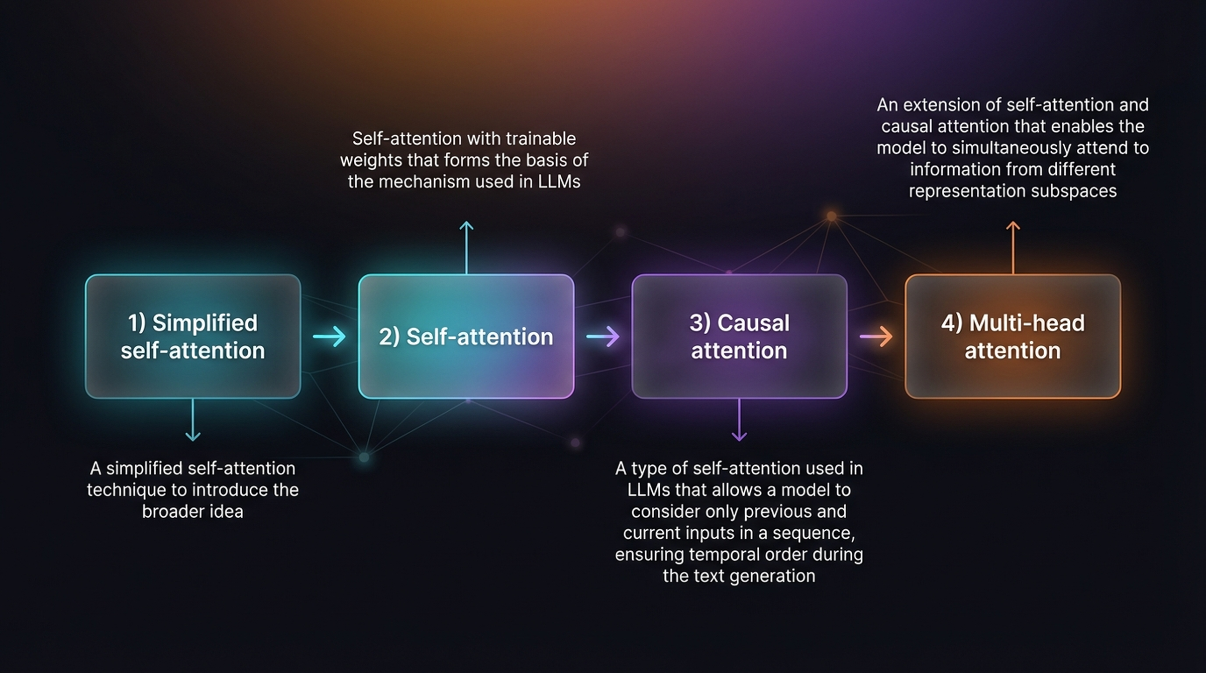
We will walk through attention in four progressive stages. Each one builds on the previous, adding one key idea at a time.
The four stages are:
- Simplified self-attention — A simplified self-attention technique to introduce the broader idea
- Self-attention — Self-attention with trainable weights that forms the basis of the mechanism used in LLMs
- Causal attention — A type of self-attention used in LLMs that allows a model to consider only previous and current inputs in a sequence, ensuring temporal order during text generation
- Multi-head attention — An extension of self-attention and causal attention that enables the model to simultaneously attend to information from different representation subspaces
2. Where Attention Fits in the LLM Pipeline
This chapter implements the attention mechanism, an important building block of GPT-like LLMs. The figure below shows where this piece fits within the larger picture of building an LLM from scratch.
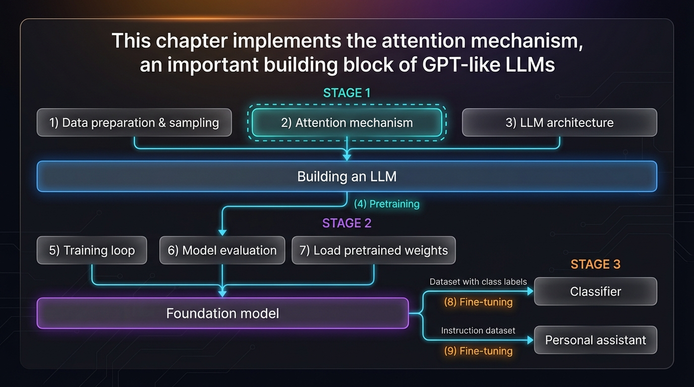
In Stage 1, the three core building blocks are: (1) Data preparation & sampling, (2) Attention mechanism (the current chapter, highlighted with a dashed border), and (3) LLM architecture. Together these components let us build the raw model that is then pretrained, evaluated, and fine-tuned in the later stages.
3. Why Attention? — The Translation Motivation
Before diving into formulas, let us understand why attention was invented. Consider translating from German to English.
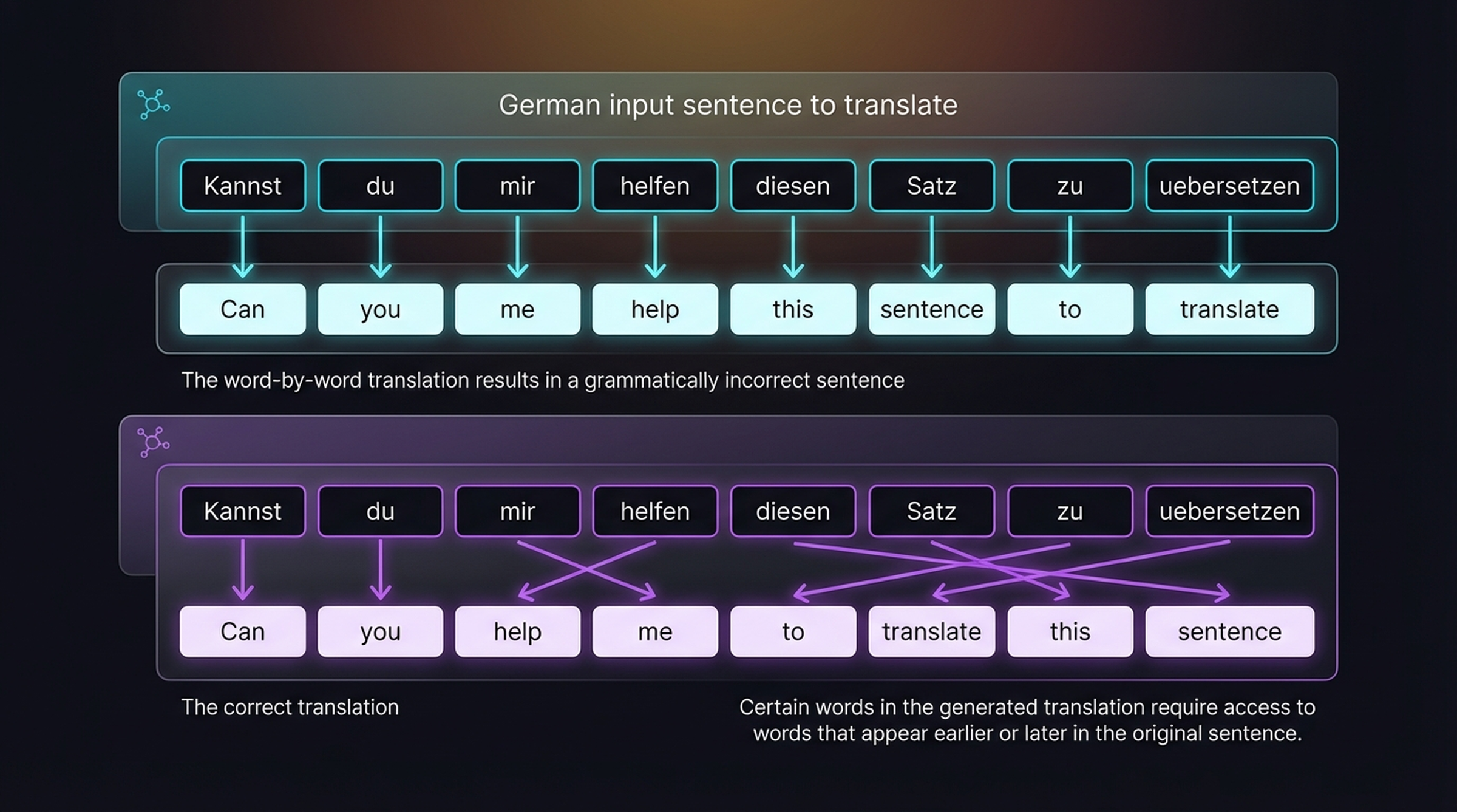
A word-by-word translation of “Kannst du mir helfen diesen Satz zu uebersetzen” gives “Can you me help this sentence to translate” — grammatically incorrect. The correct English is “Can you help me to translate this sentence.” Certain words in the generated translation require access to words that appear earlier or later in the original sentence. Attention provides exactly this capability — it lets the model selectively focus on the most relevant parts of the input when producing each output token.
From Encoder-Decoder to Self-Attention
The original attention mechanism was developed for encoder-decoder architectures used in machine translation. The encoder reads the full input sentence and compresses it into a sequence of hidden states. The decoder then generates the output one token at a time, and attention allows each decoder step to look back at all encoder hidden states, weighting them by relevance.
Modern GPT-like LLMs use a decoder-only architecture with self-attention — a variant where both the “query” and the “memory” come from the same sequence.
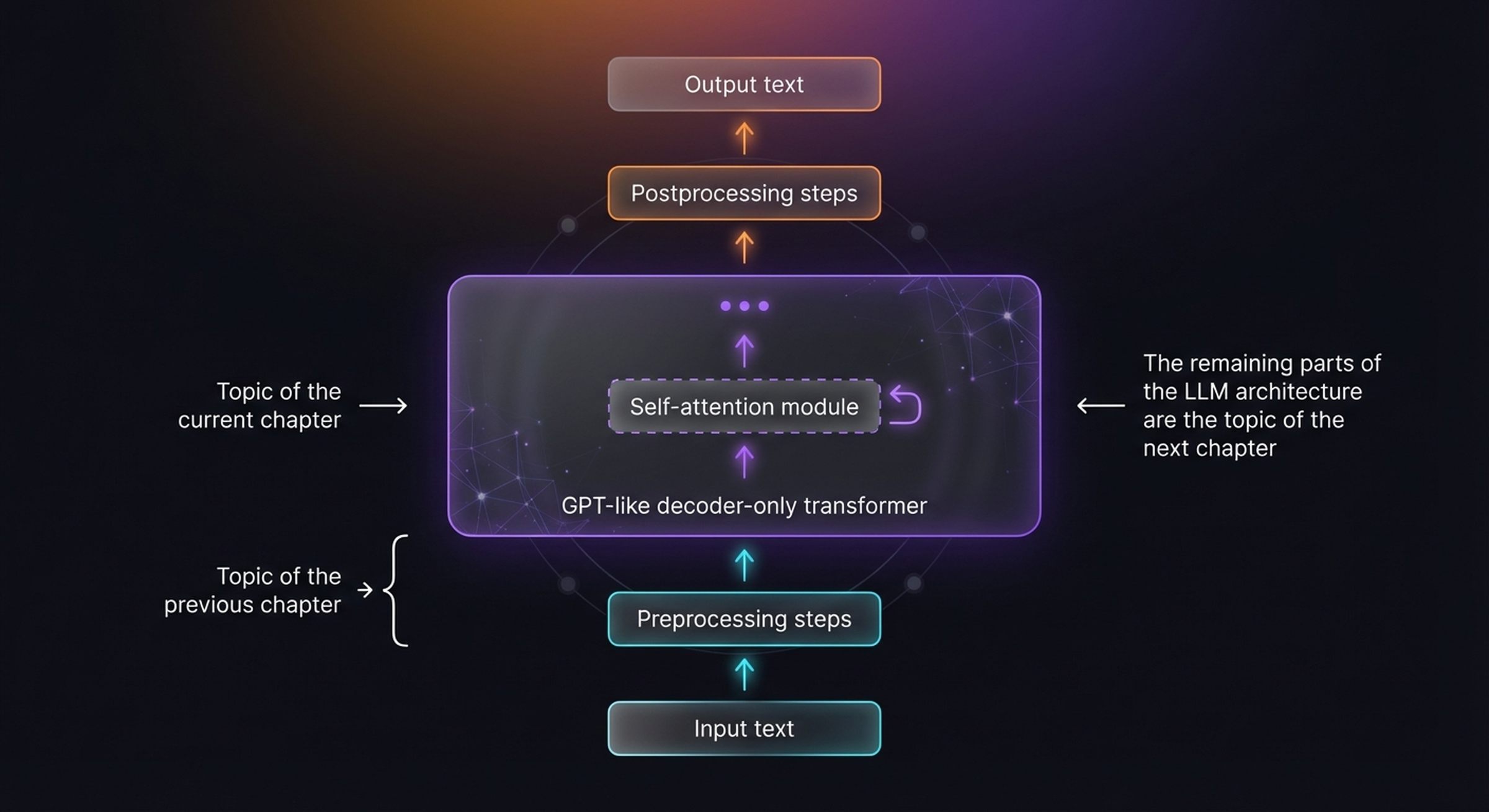
The figure above shows how a GPT-like decoder-only transformer processes text. The self-attention module (dashed box) is the core topic of this chapter. The preprocessing steps (tokenization, embeddings) were covered in the previous chapter, and the remaining architectural pieces will be the topic of the next chapter.
4. Simplified Self-Attention
We start with the simplest form of self-attention — no trainable weights, just raw dot products between input embeddings. This gives us a clean foundation to build on.
Throughout this chapter, we use the sentence “Each model learns through many rounds” (6 tokens) as our running example. Each token is represented by a 3-dimensional embedding vector:
| Token | Notation | Embedding |
|---|---|---|
| Each | \(x^{(1)}\) | \([0.31,\; 0.82,\; 0.45]\) |
| model | \(x^{(2)}\) | \([0.73,\; 0.39,\; 0.81]\) |
| learns | \(x^{(3)}\) | \([0.65,\; 0.47,\; 0.78]\) |
| through | \(x^{(4)}\) | \([0.18,\; 0.71,\; 0.29]\) |
| many | \(x^{(5)}\) | \([0.85,\; 0.22,\; 0.14]\) |
| rounds | \(x^{(6)}\) | \([0.09,\; 0.76,\; 0.62]\) |
4.1 Overview of Simplified Self-Attention
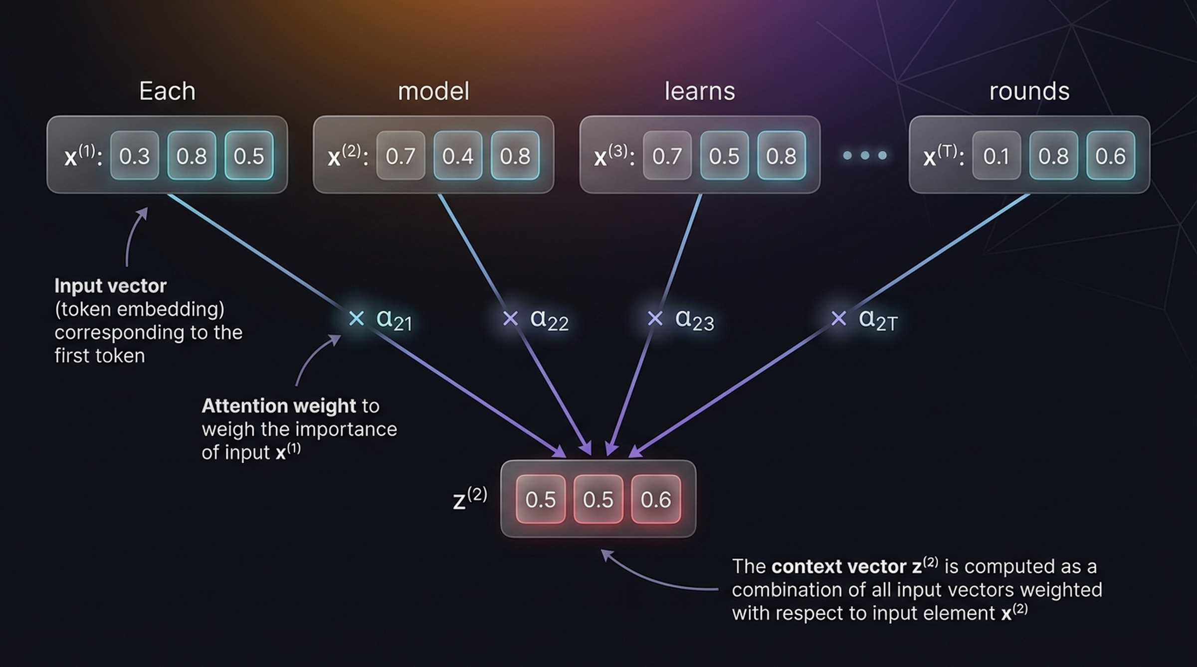
The goal: for each token, compute a context vector that is a weighted combination of all input embeddings. The weights are determined by how similar each pair of tokens is.
The context vector \(z^{(2)}\) is computed as a combination of all input vectors, weighted with respect to input element \(x^{(2)}\). Each attention weight \(\alpha_{2j}\) determines how much influence input \(x^{(j)}\) has on the output for position 2.
4.2 Step 1 — Compute Attention Scores
The attention score between the query token \(x^{(2)}\) and each input token \(x^{(j)}\) is the dot product:
\[\omega_{ij} = x^{(i)} \cdot x^{(j)} = \sum_{k=1}^{d} x^{(i)}_k \, x^{(j)}_k\]
For the query token “model” (\(x^{(2)} = [0.73, 0.39, 0.81]\)), the dot products with each input are:
\[\omega_{21} = x^{(2)} \cdot x^{(1)} = 0.73 \times 0.31 + 0.39 \times 0.82 + 0.81 \times 0.45 = 0.9\]
\[\omega_{22} = x^{(2)} \cdot x^{(2)} = 0.73^2 + 0.39^2 + 0.81^2 = 1.3\]
\[\omega_{23} = x^{(2)} \cdot x^{(3)} = 0.73 \times 0.65 + 0.39 \times 0.47 + 0.81 \times 0.78 = 1.3\]
\[\omega_{2T} = x^{(2)} \cdot x^{(6)} = 0.73 \times 0.09 + 0.39 \times 0.76 + 0.81 \times 0.62 = 0.9\]
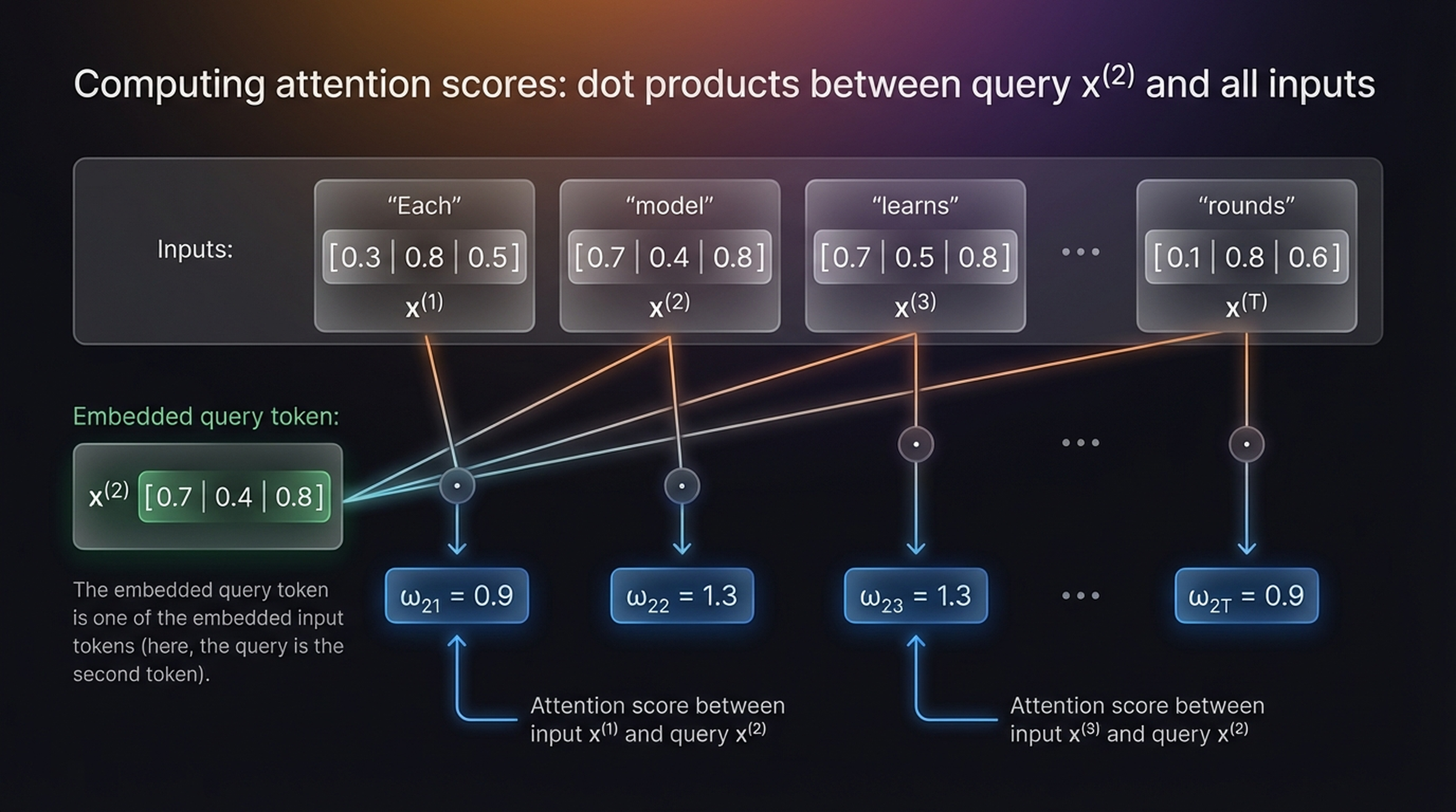
The embedded query token is one of the embedded input tokens (here, the query is the second token). Note that \(\omega_{22}\) and \(\omega_{23}\) are the highest — “model” is most similar to itself and to “learns”, which makes intuitive sense since both relate to the learning process.
4.3 Step 2 — Normalize to Attention Weights
The raw scores are not probabilities — they do not sum to 1. We normalize them using the softmax function:
\[\alpha_{ij} = \frac{\exp(\omega_{ij})}{\sum_{k=1}^{T} \exp(\omega_{ik})}\]
Applying softmax to our scores:
\[\alpha_{21} = 0.15, \quad \alpha_{22} = 0.23, \quad \alpha_{23} = 0.22, \quad \alpha_{24} = 0.12, \quad \alpha_{25} = 0.14, \quad \alpha_{2T} = 0.14\]
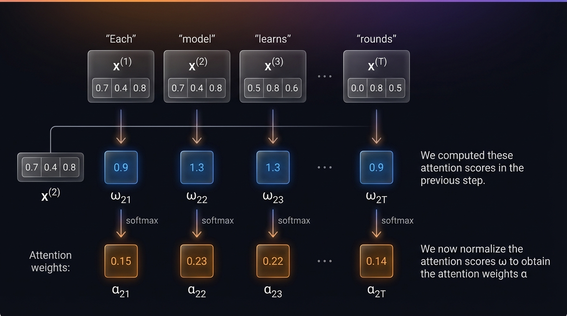
We can verify: \(0.15 + 0.23 + 0.22 + 0.12 + 0.14 + 0.14 = 1.0\) ✓. The attention weights are a normalized version of the attention scores. Notice that “model” (\(\alpha_{22}=0.23\)) and “learns” (\(\alpha_{23}=0.22\)) receive the highest weights.
4.4 Step 3 — Compute the Context Vector
The context vector is a weighted sum of all input embeddings:
\[z^{(i)} = \sum_{j=1}^{T} \alpha_{ij} \, x^{(j)}\]
Multiplying each input vector with the corresponding attention weight and summing:
\[z^{(2)} = 0.15 \cdot x^{(1)} + 0.23 \cdot x^{(2)} + 0.22 \cdot x^{(3)} + 0.12 \cdot x^{(4)} + 0.14 \cdot x^{(5)} + 0.14 \cdot x^{(6)}\]
\[z^{(2)} = [0.5,\; 0.5,\; 0.6]\]
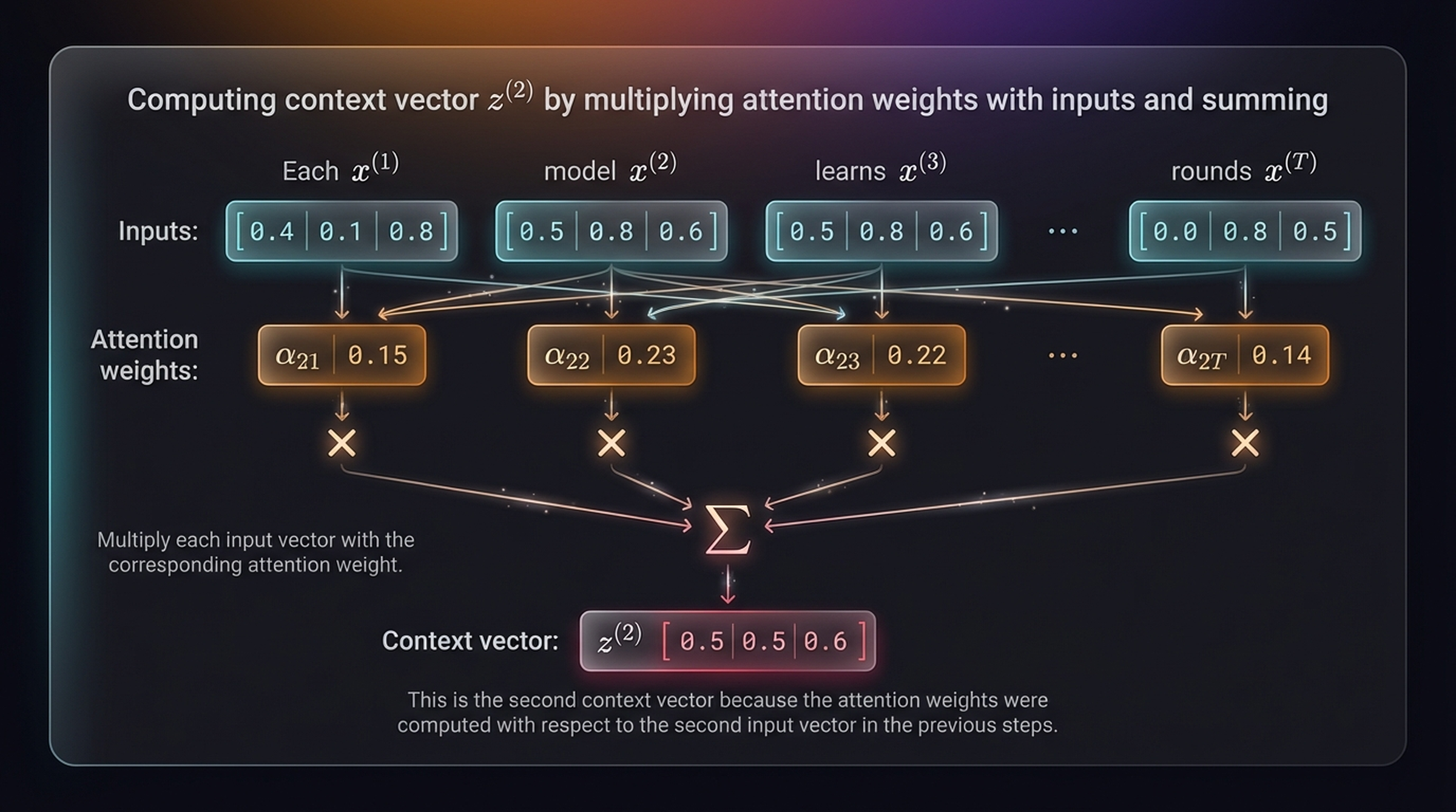
This is the second context vector because the attention weights were computed with respect to the second input vector in the previous steps.
4.5 The Full Attention Matrix
If we repeat the above three steps for every token as the query, we get a \(6 \times 6\) attention weight matrix. Each row shows how much each token attends to every other token:
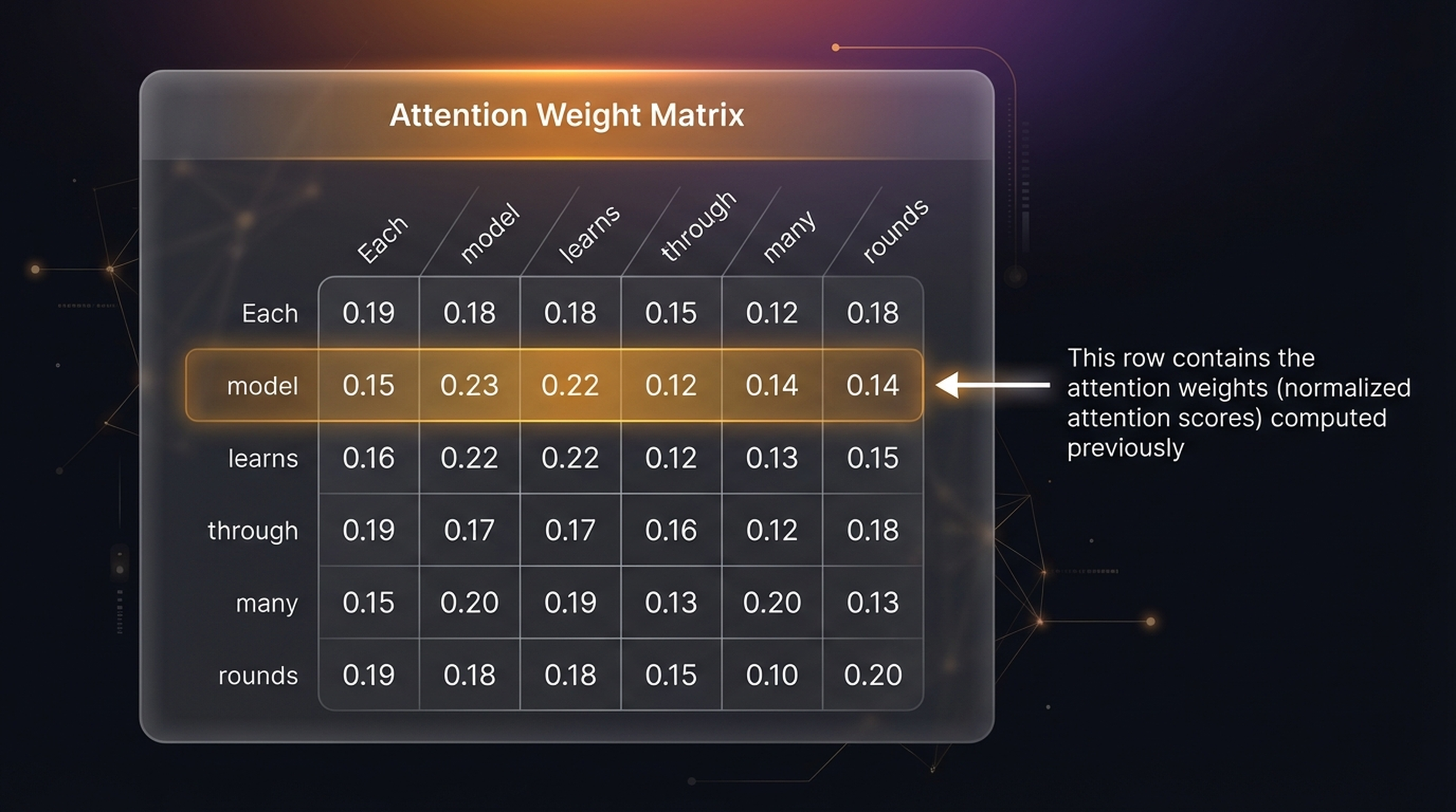
| Each | model | learns | through | many | rounds | |
|---|---|---|---|---|---|---|
| Each | 0.19 | 0.18 | 0.18 | 0.15 | 0.12 | 0.18 |
| model | 0.15 | 0.23 | 0.22 | 0.12 | 0.14 | 0.14 |
| learns | 0.16 | 0.22 | 0.22 | 0.12 | 0.13 | 0.15 |
| through | 0.19 | 0.17 | 0.17 | 0.16 | 0.12 | 0.18 |
| many | 0.15 | 0.20 | 0.19 | 0.13 | 0.20 | 0.13 |
| rounds | 0.19 | 0.18 | 0.18 | 0.15 | 0.10 | 0.20 |
The highlighted “model” row contains the attention weights we computed previously. Each row sums to 1.0.
4.6 Summary — Three Steps of Simplified Self-Attention
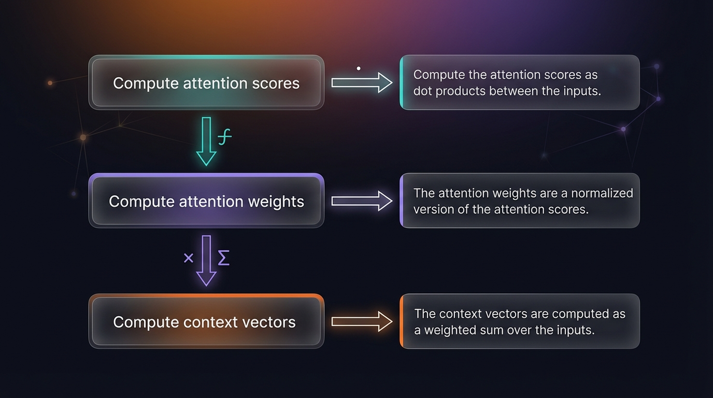
- Compute attention scores — Compute the attention scores as dot products between the inputs
- Compute attention weights — The attention weights are a normalized version of the attention scores
- Compute context vectors — The context vectors are computed as a weighted sum over the inputs
5. Self-Attention with Trainable Weights (Q, K, V)
The simplified self-attention has no learnable parameters — the attention scores are fully determined by the fixed input embeddings. To make the mechanism learnable, we introduce three weight matrices: \(W_q\) (query), \(W_k\) (key), and \(W_v\) (value).
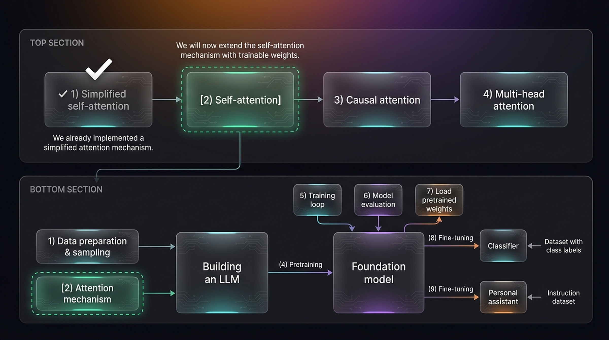
We already implemented a simplified attention mechanism. We will now extend the self-attention mechanism with trainable weights.
Why Three Separate Projections?
In simplified self-attention, each token plays all three roles at once — it is simultaneously the thing asking the question, the thing being compared against, and the thing contributing information to the output. This is limiting because what makes a token relevant to another token is not necessarily the same as what information that token should contribute.
Think of it like a library analogy. You walk in with a query — “I need something about machine learning.” The librarian compares your query against the key on each book’s catalog card — the title, subject tags, and summary that describe what the book is about. Once the best matches are found, you do not read the catalog cards — you read the actual values, the book contents themselves.
The query (\(q\)) encodes “what am I looking for?”, the key (\(k\)) encodes “what do I contain?”, and the value (\(v\)) encodes “what information do I actually provide if selected?”. By learning three separate projections, the model decouples these three roles so that the matching criterion (query vs key) can be completely independent from the information being passed (value).
For example, consider the sentence “The cat sat on the mat because it was tired.” When processing the word “it”, the query projection learns to encode something like “looking for an animate noun”, the key projection for “cat” learns to encode “I am an animate noun”, and the value projection for “cat” provides the actual semantic content — the meaning of “cat” — that gets blended into the context vector for “it”. Without separate projections, the model would be forced to use the same embedding for matching and for information transfer, which severely limits its expressiveness.
Why Does the Dot Product Work for Measuring Relevance?
The dot product \(q \cdot k = \sum_i q_i k_i\) measures how well two vectors align in the projected space. When two vectors point in the same direction, their dot product is large and positive — they are “similar” in whatever abstract feature space the weight matrices have learned. When they are orthogonal, the dot product is zero — they are unrelated. During training, the weight matrices \(W_q\) and \(W_k\) learn to project tokens into a space where semantically relevant pairs produce high dot products.
This is computationally elegant because \(Q K^T\) computes all pairwise attention scores in a single matrix multiplication — no loops, no conditionals, just one highly optimized operation that GPUs execute extremely efficiently.
5.1 Query, Key, and Value Projections
Each input token is projected into three different spaces using the learnable weight matrices:
\[q^{(i)} = x^{(i)} \cdot W_q, \qquad k^{(i)} = x^{(i)} \cdot W_k, \qquad v^{(i)} = x^{(i)} \cdot W_v\]
where \(W_q, W_k, W_v \in \mathbb{R}^{d_{in} \times d_{out}}\). In our example, \(d_{in} = 3\) and \(d_{out} = 2\), so each projection reduces the dimensionality from 3 to 2.
The weight matrices used throughout this section are:
\[W_q = \begin{bmatrix} 0.5 & 0.8 \\ 0.3 & 0.1 \\ 0.2 & 0.6 \end{bmatrix}, \quad W_k = \begin{bmatrix} 0.4 & 0.3 \\ 0.1 & 0.7 \\ 0.5 & 0.2 \end{bmatrix}, \quad W_v = \begin{bmatrix} 0.2 & 0.5 \\ 0.3 & 0.1 \\ 0.4 & 0.3 \end{bmatrix}\]
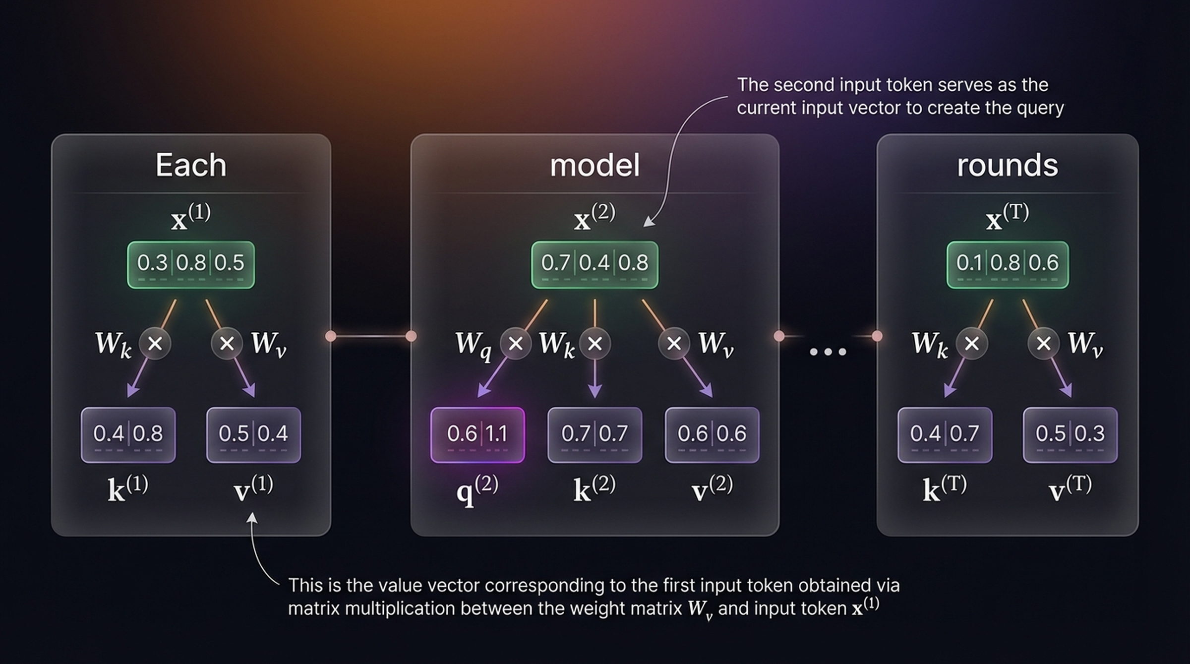
For the query token “model” (\(x^{(2)} = [0.73, 0.39, 0.81]\)):
\[q^{(2)} = x^{(2)} \cdot W_q = [0.73, 0.39, 0.81] \cdot \begin{bmatrix} 0.5 & 0.8 \\ 0.3 & 0.1 \\ 0.2 & 0.6 \end{bmatrix} = [0.6,\; 1.1]\]
The key and value vectors for representative tokens:
| Token | Key \(k^{(i)}\) | Value \(v^{(i)}\) |
|---|---|---|
| Each (\(x^{(1)}\)) | \([0.4,\; 0.8]\) | \([0.5,\; 0.4]\) |
| model (\(x^{(2)}\)) | \([0.7,\; 0.7]\) | \([0.6,\; 0.6]\) |
| rounds (\(x^{(T)}\)) | \([0.4,\; 0.7]\) | \([0.5,\; 0.3]\) |
The second input token serves as the current input vector to create the query.
5.2 Attention Scores via Dot Products
The unnormalized attention scores are computed as dot products between the query and each key vector:
\[\omega_{ij} = q^{(i)} \cdot k^{(j)}\]
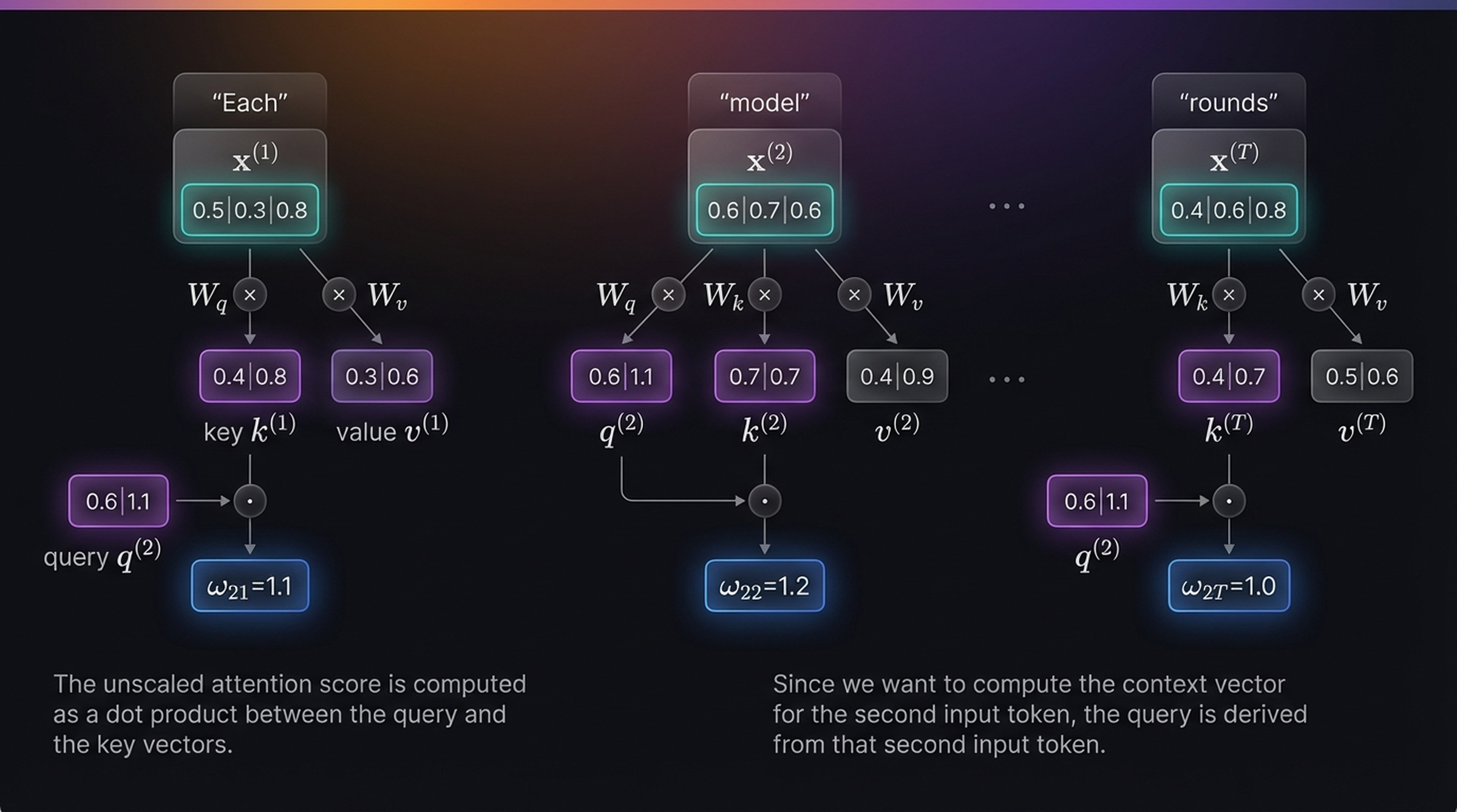
\[\omega_{21} = q^{(2)} \cdot k^{(1)} = [0.6,\; 1.1] \cdot [0.4,\; 0.8] = 0.6 \times 0.4 + 1.1 \times 0.8 = 1.1\]
\[\omega_{22} = q^{(2)} \cdot k^{(2)} = [0.6,\; 1.1] \cdot [0.7,\; 0.7] = 0.6 \times 0.7 + 1.1 \times 0.7 = 1.2\]
\[\omega_{2T} = q^{(2)} \cdot k^{(T)} = [0.6,\; 1.1] \cdot [0.4,\; 0.7] = 0.6 \times 0.4 + 1.1 \times 0.7 = 1.0\]
The unscaled attention score is computed as a dot product between the query and the key vectors.
5.3 Scaled Dot-Product Attention
In practice, the scores are scaled by \(\sqrt{d_k}\) to prevent the softmax from becoming too peaked when the dimensionality is large:
\[\alpha_{ij} = \text{softmax}\!\left(\frac{q^{(i)} \cdot k^{(j)}}{\sqrt{d_k}}\right)\]
where \(d_k\) is the dimensionality of the key vectors (\(d_k = d_{out} = 2\) in our example).
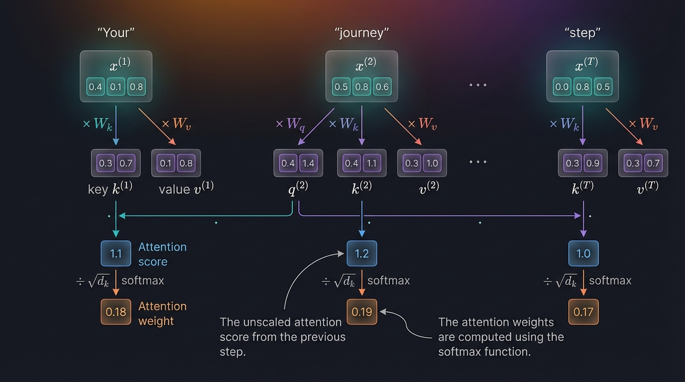
After scaling by \(\sqrt{2} \approx 1.41\) and applying softmax:
\[\alpha_{21} = 0.18, \quad \alpha_{22} = 0.19, \quad \alpha_{2T} = 0.17\]
The attention weights are computed using the softmax function. Notice the weights are more uniform than in simplified attention — this is because the scaling prevents extreme softmax outputs.
5.4 Context Vector with Trainable Attention
The final step multiplies each value vector by its attention weight and sums:
\[z^{(i)} = \sum_{j=1}^{T} \alpha_{ij} \, v^{(j)}\]
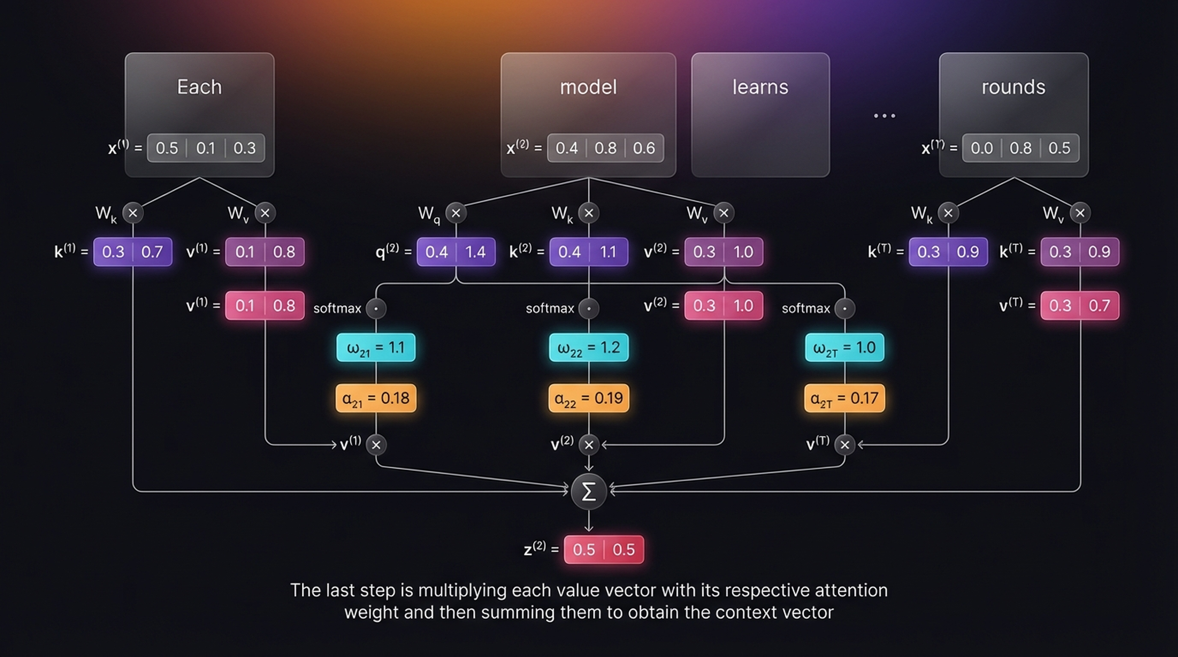
\[z^{(2)} = 0.18 \cdot v^{(1)} + 0.19 \cdot v^{(2)} + \cdots + 0.17 \cdot v^{(T)} = [0.5,\; 0.5]\]
The last step is multiplying each value vector with its respective attention weight and then summing them to obtain the context vector.
5.5 The Full Self-Attention Pipeline
Putting it all together into the SelfAttention class, the full pipeline for all 6 tokens is:
\[X \in \mathbb{R}^{n \times d_{in}} \xrightarrow{\times W_q} Q \in \mathbb{R}^{n \times d_{out}}, \quad \xrightarrow{\times W_k} K \in \mathbb{R}^{n \times d_{out}}, \quad \xrightarrow{\times W_v} V \in \mathbb{R}^{n \times d_{out}}\]
\[\text{Attention}(Q, K, V) = \text{softmax}\!\left(\frac{Q \, K^T}{\sqrt{d_k}}\right) V\]
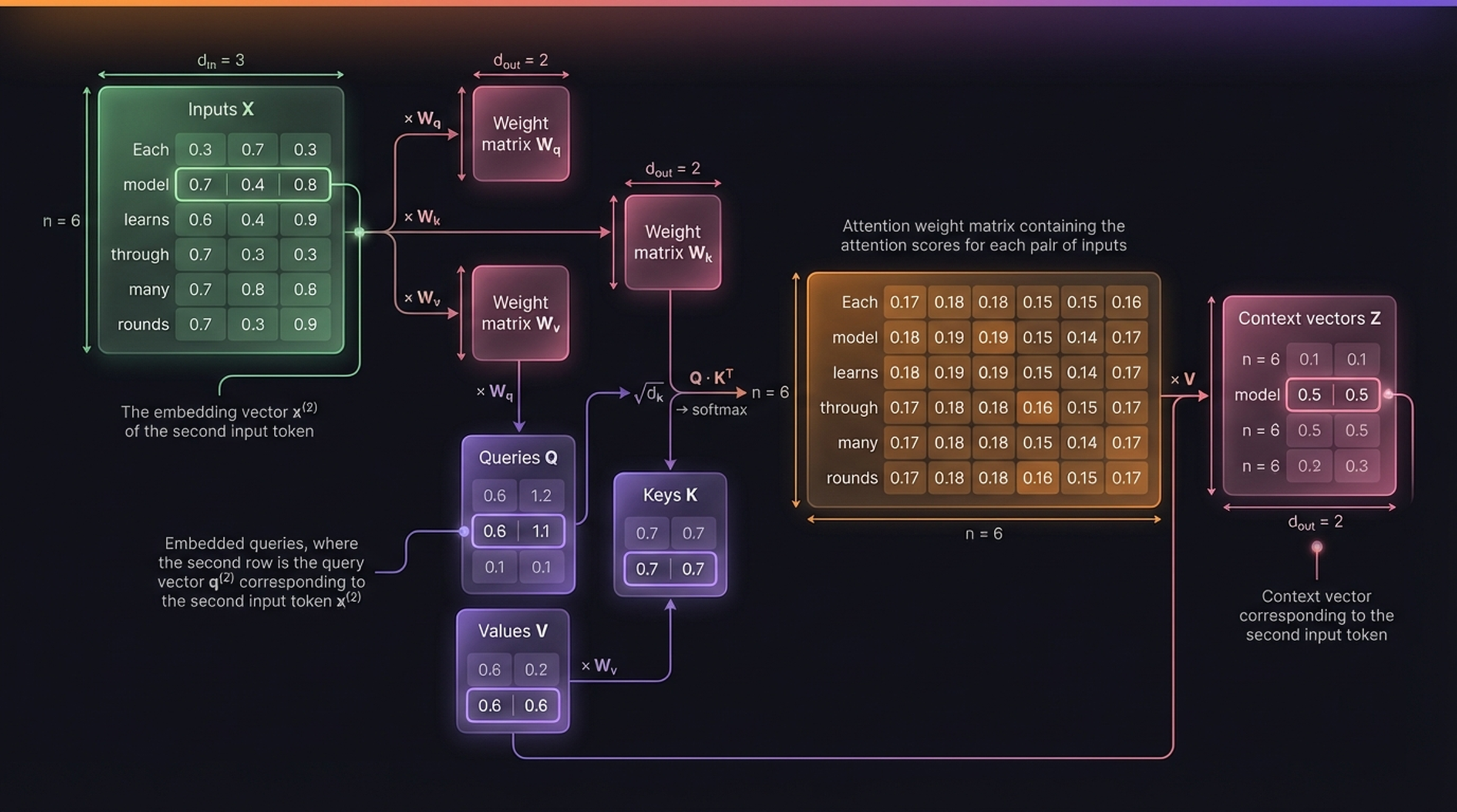
The full \(6 \times 6\) attention weight matrix with trainable weights:
| Each | model | learns | through | many | rounds | |
|---|---|---|---|---|---|---|
| Each | 0.17 | 0.18 | 0.18 | 0.15 | 0.15 | 0.16 |
| model | 0.18 | 0.19 | 0.19 | 0.15 | 0.14 | 0.17 |
| learns | 0.18 | 0.19 | 0.19 | 0.15 | 0.14 | 0.17 |
| through | 0.17 | 0.18 | 0.18 | 0.16 | 0.15 | 0.17 |
| many | 0.17 | 0.18 | 0.18 | 0.15 | 0.14 | 0.17 |
| rounds | 0.17 | 0.18 | 0.18 | 0.16 | 0.15 | 0.17 |
The context vector for “model” is \(z^{(2)} = [0.5,\; 0.5]\), now in \(\mathbb{R}^{d_{out}} = \mathbb{R}^2\) rather than the original \(\mathbb{R}^3\).
6. Causal Attention — Masking and Dropout
In autoregressive language models like GPT, a token should only attend to previous tokens and itself — never to future tokens. This is enforced with a causal mask.
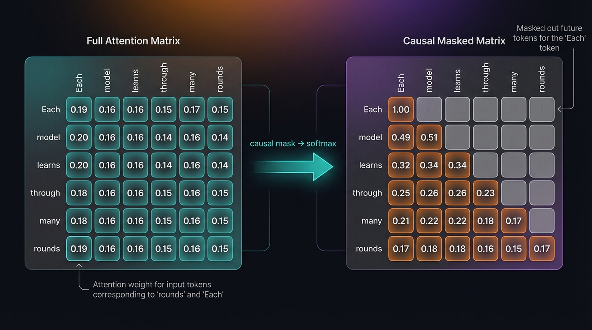
6.1 The Causal Mask
The causal mask zeros out the upper triangle of the attention matrix (future tokens) and renormalizes each row so the weights still sum to 1:
\[\text{CausalMask}_{ij} = \begin{cases} \alpha_{ij} & \text{if } j \leq i \\ 0 & \text{if } j > i \end{cases} \quad \text{then renormalize each row}\]
The causal-masked attention weights for our sentence:
| Each | model | learns | through | many | rounds | |
|---|---|---|---|---|---|---|
| Each | 1.00 | — | — | — | — | — |
| model | 0.49 | 0.51 | — | — | — | — |
| learns | 0.32 | 0.34 | 0.34 | — | — | — |
| through | 0.25 | 0.26 | 0.26 | 0.23 | — | — |
| many | 0.21 | 0.22 | 0.22 | 0.18 | 0.17 | — |
| rounds | 0.17 | 0.18 | 0.18 | 0.16 | 0.15 | 0.17 |
The first token “Each” can only attend to itself (weight = 1.0). The last token “rounds” can attend to all tokens. Each row sums to 1.0 after renormalization.
6.2 Naive vs Efficient Masking
There are two approaches to implementing the causal mask:
Naive approach (3 steps):
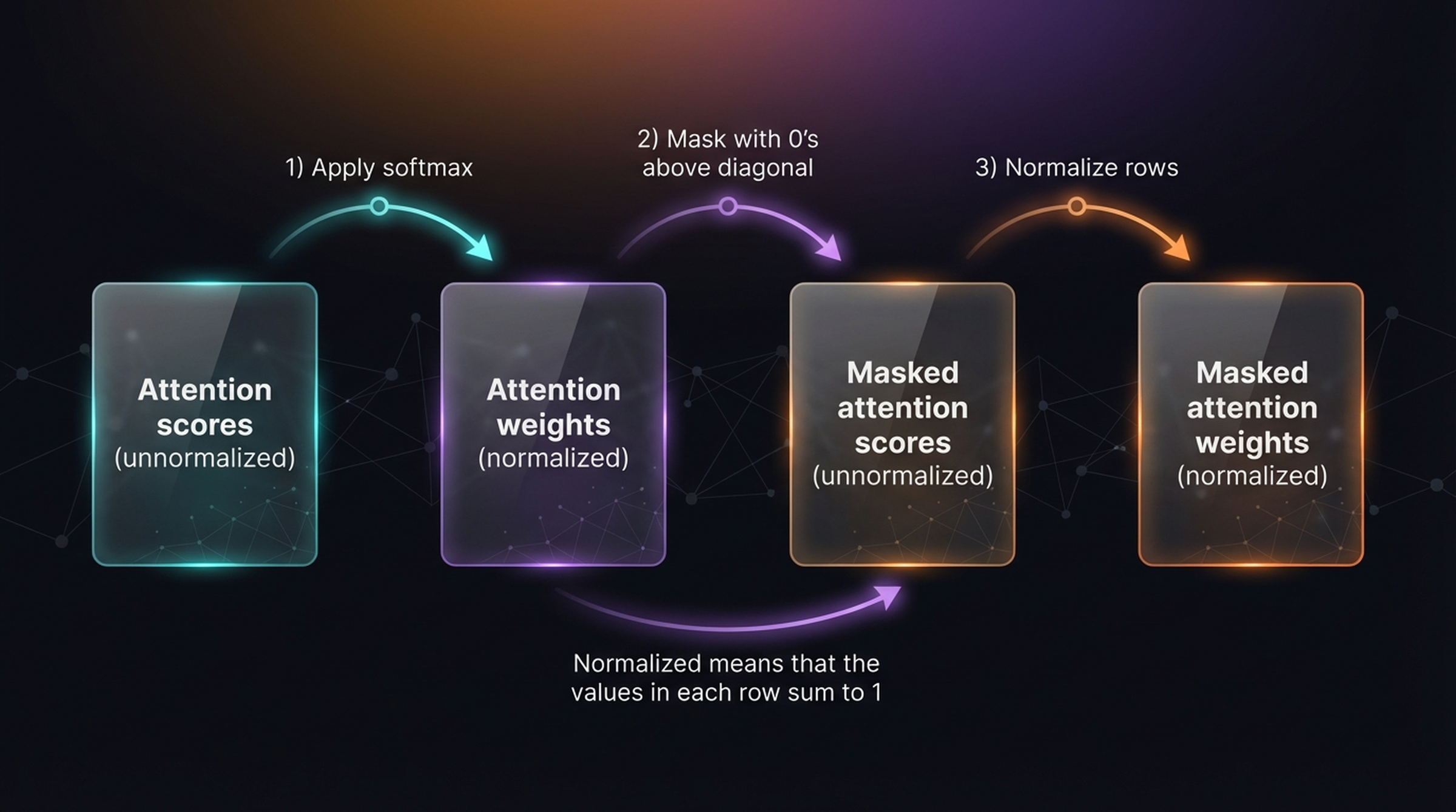
- Apply softmax to the unnormalized attention scores
- Mask with 0s above the diagonal
- Renormalize rows so they sum to 1
Efficient approach (2 steps):
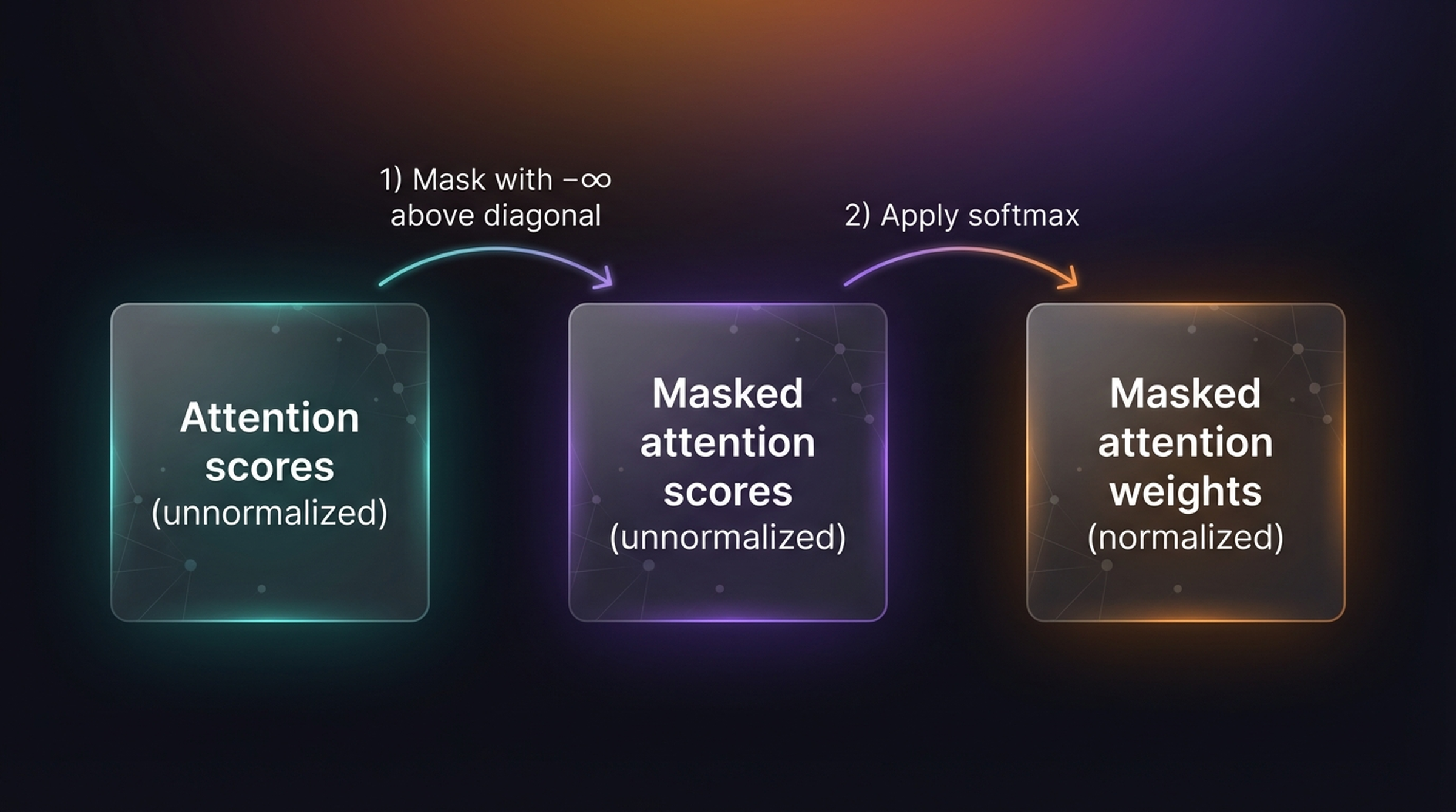
- Mask with \(-\infty\) above the diagonal
- Apply softmax (which converts \(-\infty \to 0\) automatically)
The efficient approach is preferred because it avoids the renormalization step — since \(\exp(-\infty) = 0\), the softmax naturally gives zero weight to masked positions.
In mathematical notation, the efficient approach is:
\[\text{CausalAttention}(Q, K, V) = \text{softmax}\!\left(\frac{Q K^T + M}{\sqrt{d_k}}\right) V\]
where \(M\) is the mask matrix with \(M_{ij} = 0\) if \(j \leq i\) and \(M_{ij} = -\infty\) if \(j > i\).
6.3 Dropout on Attention Weights
After causal masking, we optionally apply dropout to the attention weights during training. This randomly zeros out some attention connections, forcing the model to not over-rely on any single token:
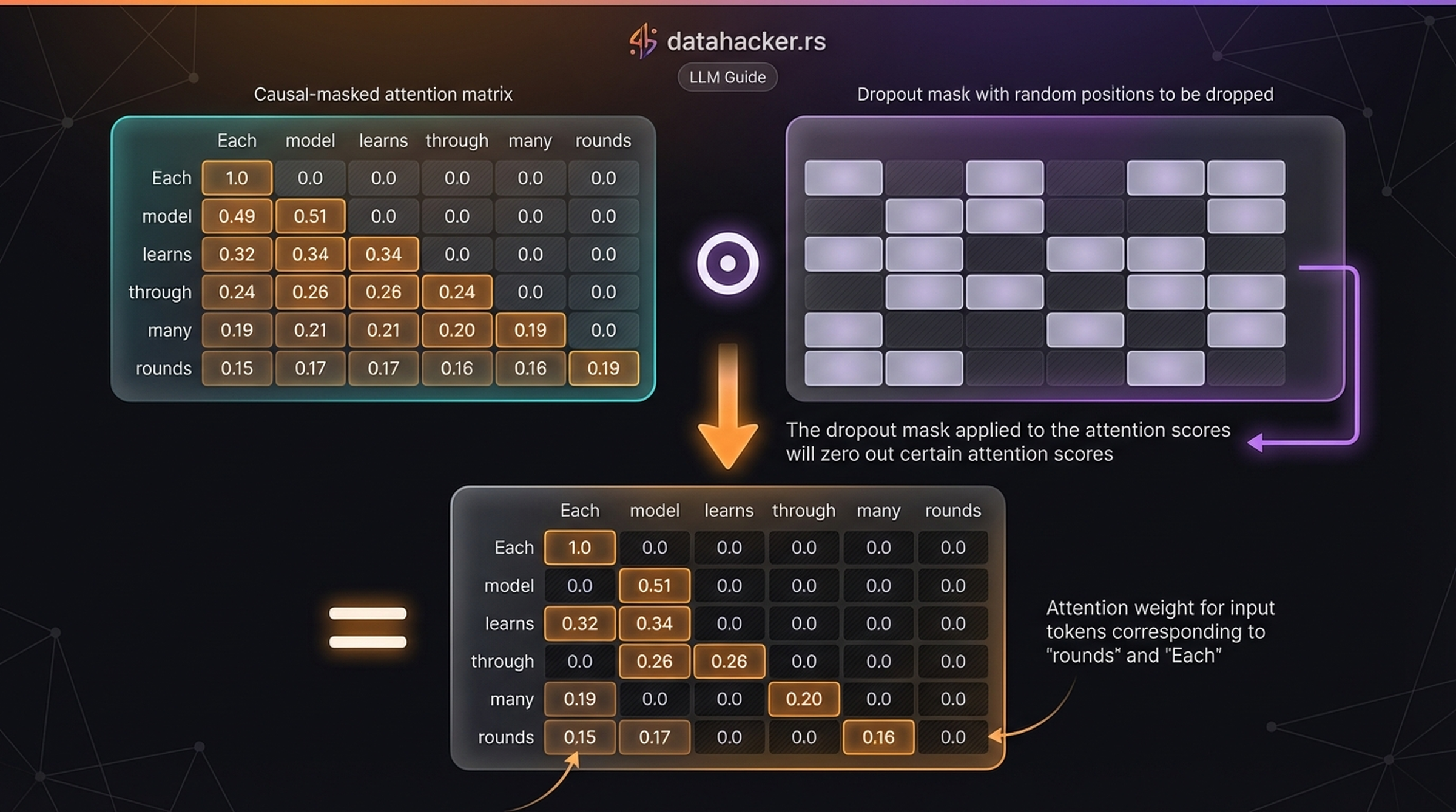
The dropout mask is a random binary matrix where each entry is 0 with probability \(p\) (the dropout rate). The remaining non-zero entries are scaled by \(\frac{1}{1-p}\) to keep the expected value unchanged.
6.4 Progress Check
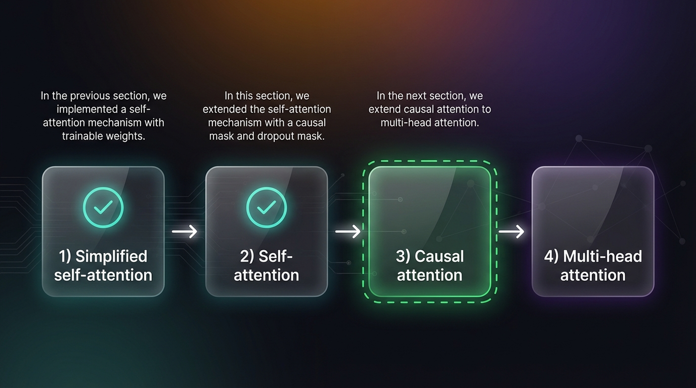
In the previous section, we implemented a self-attention mechanism with trainable weights. In this section, we extended the self-attention mechanism with a causal mask and dropout mask. In the next section, we extend causal attention to multi-head attention.
7. Multi-Head Attention — Parallel Subspaces
Single-head attention compresses all information into one set of attention weights. Multi-head attention runs multiple attention computations in parallel, each learning to focus on different aspects of the input (syntax, semantics, position, etc.).
Why Multiple Heads?
Consider the sentence “The animal didn’t cross the street because it was too wide.” The word “it” needs to resolve two very different types of information simultaneously — it needs to figure out what “it” refers to (the street, not the animal), and it needs to understand why that referent matters (because width is a property of streets). A single attention head would be forced to compromise — it can either focus on coreference resolution or on semantic reasoning, but cramming both into one set of weights leads to a blurred, suboptimal representation.
Multi-head attention solves this by giving the model parallel “lenses” through which to view the same input. In practice, researchers have observed that different heads in trained models specialize in remarkably distinct patterns. For example, in the original “Attention Is All You Need” transformer, some heads learned to track syntactic dependencies (subject-verb agreement across long distances), others learned positional patterns (always attending to the previous or next token), and still others captured semantic similarity (attending to synonyms or related concepts). One famous finding by Clark et al. (2019) showed that specific heads in BERT almost perfectly replicate the dependency parse tree — one head for direct objects, another for possessive pronouns, another for prepositional attachments.
This specialization has a direct impact on model quality. The GPT line of models uses between 12 heads (GPT-2 small) and 96 heads (GPT-3), and ablation studies consistently show that removing heads degrades performance — particularly on tasks requiring multiple types of reasoning within a single sentence, such as question answering, summarization, and code generation.
A concrete intuition: imagine reading the sentence “Each model learns through many rounds” while simultaneously tracking (a) which words are semantically related (“model”—“learns”—“rounds”), (b) which words are syntactically linked (“Each” modifies “model”), and (c) which words are positionally adjacent. No single weighting scheme can capture all three at once, but three separate heads can — and their combined output gives downstream layers access to all three perspectives.
7.1 Architecture with 2 Heads
Instead of one set of weight matrices \((W_q, W_k, W_v)\), we use two: \((W_{q1}, W_{k1}, W_{v1})\) and \((W_{q2}, W_{k2}, W_{v2})\).
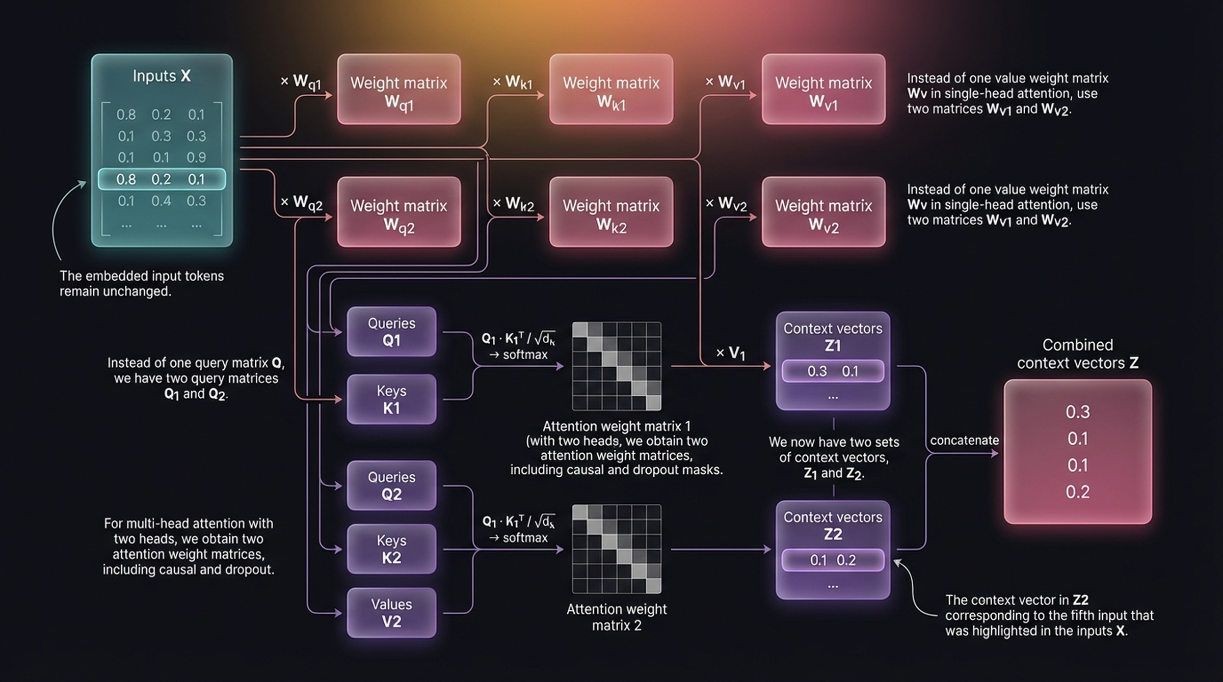
Each head produces its own set of context vectors. For the 5th input token “many” (\(x^{(5)} = [0.85, 0.22, 0.14]\)):
\[Z_1^{(5)} = [0.3,\; 0.1], \quad Z_2^{(5)} = [0.1,\; 0.2]\]
The outputs of both heads are concatenated:
\[Z^{(5)} = [Z_1^{(5)} \;|\; Z_2^{(5)}] = [0.3,\; 0.1,\; 0.1,\; 0.2]\]
7.2 Dimensionality
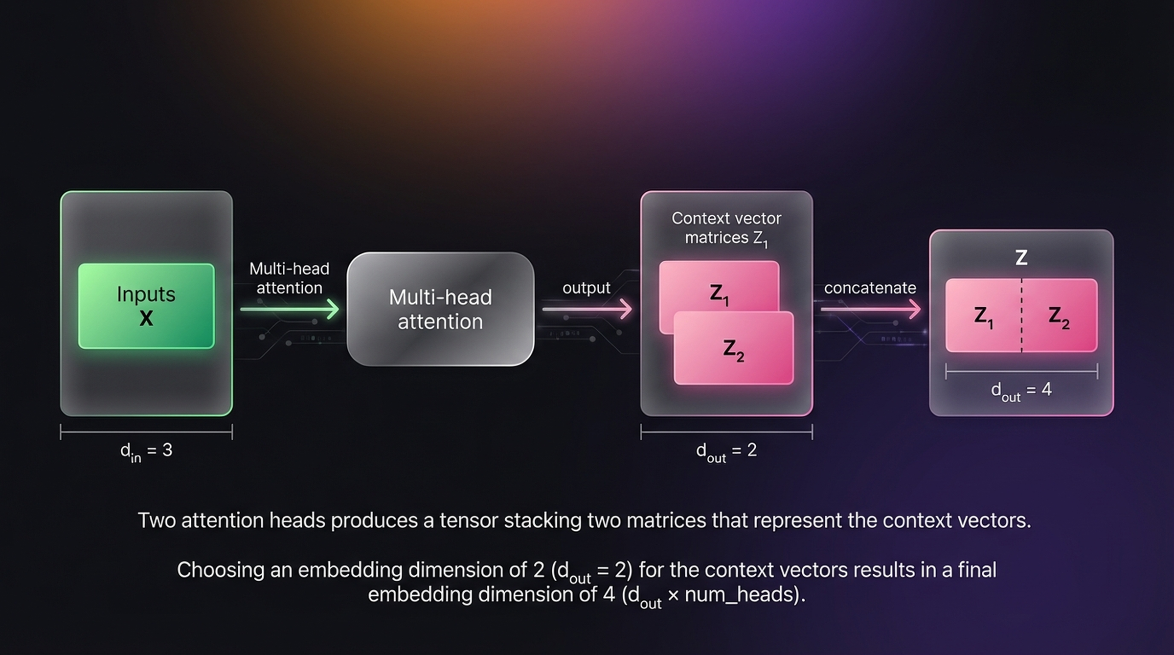
Choosing an embedding dimension of \(d_{out} = 2\) for the context vectors, with 2 attention heads, results in a final embedding dimension of \(d_{out} \times \text{num\_heads} = 2 \times 2 = 4\). In general:
\[d_{\text{final}} = d_{\text{head}} \times h\]
where \(h\) is the number of heads and \(d_{\text{head}} = d_{\text{model}} / h\).
7.3 Efficient Implementation — One Large Matrix Instead of Many Small Ones
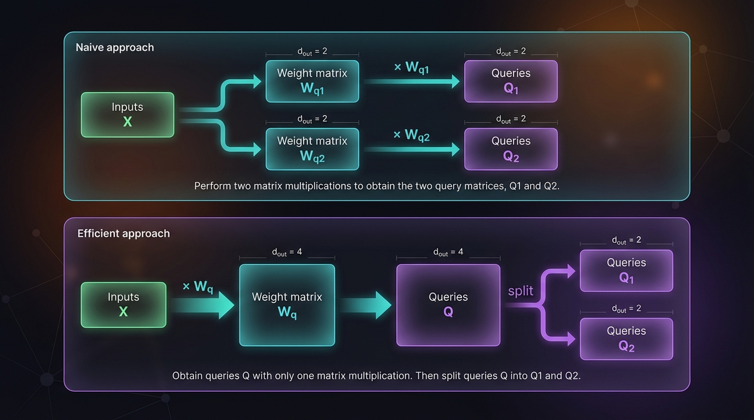
Naive approach: Perform \(h\) separate matrix multiplications, one per head:
\[Q_1 = X \cdot W_{q1}, \quad Q_2 = X \cdot W_{q2}\]
Efficient approach: Concatenate weight matrices into one large matrix, perform a single matrix multiplication, then split:
\[Q = X \cdot W_q \quad \text{where } W_q \in \mathbb{R}^{d_{in} \times (h \cdot d_{out})}\]
\[Q_1, Q_2 = \text{split}(Q)\]
The efficient approach uses one matrix multiplication instead of two, which is significantly faster on GPUs due to better memory access patterns.
8. Compact Code Implementations
Below are compact, editable PyTorch implementations for each attention type. The numerical values match the figures above so you can verify each step.
8.1 Simplified Self-Attention
import torch
import torch.nn.functional as F

# Input embeddings: "Each model learns through many rounds"
X = torch.tensor([
    [0.31, 0.82, 0.45],  # Each    x(1)
    [0.73, 0.39, 0.81],  # model   x(2) ← query
    [0.65, 0.47, 0.78],  # learns  x(3)
    [0.18, 0.71, 0.29],  # through x(4)
    [0.85, 0.22, 0.14],  # many    x(5)
    [0.09, 0.76, 0.62],  # rounds  x(6)
])

# Step 1: Attention scores (dot products)
omega = X @ X.T  # (6, 6)
print("Attention scores (query=x(2)):", omega[1].round(decimals=1))
# → tensor([0.9, 1.3, 1.3, 0.6, 0.8, 0.9])

# Step 2: Normalize with softmax
alpha = F.softmax(omega, dim=-1)  # (6, 6)
print("Attention weights (row 'model'):", alpha[1].round(decimals=2))
# → tensor([0.15, 0.23, 0.22, 0.12, 0.14, 0.14])

# Step 3: Context vectors
Z = alpha @ X  # (6, 3)
print("Context vector z(2):", Z[1].round(decimals=1))
# → tensor([0.5, 0.5, 0.6])
8.2 Self-Attention with Trainable Weights
import torch
import torch.nn.functional as F

X = torch.tensor([
    [0.31, 0.82, 0.45],  # Each
    [0.73, 0.39, 0.81],  # model   ← query
    [0.65, 0.47, 0.78],  # learns
    [0.18, 0.71, 0.29],  # through
    [0.85, 0.22, 0.14],  # many
    [0.09, 0.76, 0.62],  # rounds
])

d_in, d_out = 3, 2

# Trainable weight matrices (3×2)
Wq = torch.tensor([[0.5, 0.8], [0.3, 0.1], [0.2, 0.6]])
Wk = torch.tensor([[0.4, 0.3], [0.1, 0.7], [0.5, 0.2]])
Wv = torch.tensor([[0.2, 0.5], [0.3, 0.1], [0.4, 0.3]])

# Project to Q, K, V
Q = X @ Wq  # (6, 2)
K = X @ Wk  # (6, 2)
V = X @ Wv  # (6, 2)

print("q(2):", Q[1].round(decimals=1))  # → [0.6, 1.1]
print("k(2):", K[1].round(decimals=1))  # → [0.7, 0.7]
print("v(2):", V[1].round(decimals=1))  # → [0.6, 0.6]

# Scaled dot-product attention
d_k = d_out
omega = Q @ K.T / (d_k ** 0.5)       # (6, 6)
alpha = F.softmax(omega, dim=-1)       # (6, 6)
Z = alpha @ V                          # (6, 2)

print("Attention scores (query=x(2)):", (Q[1] @ K.T)[..., :3].round(decimals=1))
# → ω₂₁=1.1, ω₂₂=1.2, ...

print("Attention weights (row 'model'):", alpha[1].round(decimals=2))
# → tensor([0.18, 0.19, 0.19, 0.15, 0.14, 0.17])

print("Context vector z(2):", Z[1].round(decimals=1))
# → tensor([0.5, 0.5])
8.3 Causal Attention with Dropout
import torch
import torch.nn.functional as F

X = torch.tensor([
    [0.31, 0.82, 0.45],  [0.73, 0.39, 0.81],
    [0.65, 0.47, 0.78],  [0.18, 0.71, 0.29],
    [0.85, 0.22, 0.14],  [0.09, 0.76, 0.62],
])

Wq = torch.tensor([[0.5, 0.8], [0.3, 0.1], [0.2, 0.6]])
Wk = torch.tensor([[0.4, 0.3], [0.1, 0.7], [0.5, 0.2]])
Wv = torch.tensor([[0.2, 0.5], [0.3, 0.1], [0.4, 0.3]])

Q, K, V = X @ Wq, X @ Wk, X @ Wv
d_k = 2
n = X.shape[0]

# Scores
omega = Q @ K.T / (d_k ** 0.5)

# Causal mask: -inf above diagonal (efficient approach)
mask = torch.triu(torch.ones(n, n), diagonal=1).bool()
omega = omega.masked_fill(mask, float('-inf'))

# Softmax (exp(-inf) → 0 automatically)
alpha = F.softmax(omega, dim=-1)

print("Causal attention weights:")
print(alpha.round(decimals=2))
# Each:    [1.00, 0.00, 0.00, 0.00, 0.00, 0.00]
# model:   [0.49, 0.51, 0.00, 0.00, 0.00, 0.00]
# learns:  [0.32, 0.34, 0.34, 0.00, 0.00, 0.00]
# through: [0.25, 0.26, 0.26, 0.23, 0.00, 0.00]
# many:    [0.21, 0.22, 0.22, 0.18, 0.17, 0.00]
# rounds:  [0.17, 0.18, 0.18, 0.16, 0.15, 0.17]

# Optional dropout during training
dropout = torch.nn.Dropout(p=0.1)
alpha_dropped = dropout(alpha)

Z = alpha_dropped @ V  # (6, 2)
8.4 Multi-Head Attention
import torch
import torch.nn as nn
import torch.nn.functional as F

class MultiHeadAttention(nn.Module):
    def __init__(self, d_in, d_out, num_heads, dropout=0.1):
        super().__init__()
        assert d_out % num_heads == 0
        self.num_heads = num_heads
        self.d_head = d_out // num_heads

        # Single large projection (efficient approach)
        self.W_q = nn.Linear(d_in, d_out, bias=False)
        self.W_k = nn.Linear(d_in, d_out, bias=False)
        self.W_v = nn.Linear(d_in, d_out, bias=False)
        self.dropout = nn.Dropout(dropout)

    def forward(self, X):
        B, n, _ = X.shape

        # Project and split into heads
        Q = self.W_q(X).view(B, n, self.num_heads, self.d_head).transpose(1, 2)
        K = self.W_k(X).view(B, n, self.num_heads, self.d_head).transpose(1, 2)
        V = self.W_v(X).view(B, n, self.num_heads, self.d_head).transpose(1, 2)
        # Q, K, V: (B, num_heads, n, d_head)

        # Scaled dot-product attention with causal mask
        omega = Q @ K.transpose(-2, -1) / (self.d_head ** 0.5)
        mask = torch.triu(torch.ones(n, n, device=X.device), diagonal=1).bool()
        omega = omega.masked_fill(mask, float('-inf'))
        alpha = self.dropout(F.softmax(omega, dim=-1))

        # Weighted sum and concatenate heads
        Z = alpha @ V                              # (B, num_heads, n, d_head)
        Z = Z.transpose(1, 2).contiguous()         # (B, n, num_heads, d_head)
        Z = Z.view(B, n, self.num_heads * self.d_head)  # (B, n, d_out)
        return Z

# Usage
d_in, d_out, num_heads = 3, 4, 2
mha = MultiHeadAttention(d_in, d_out, num_heads, dropout=0.0)

X = torch.tensor([
    [0.31, 0.82, 0.45],  [0.73, 0.39, 0.81],
    [0.65, 0.47, 0.78],  [0.18, 0.71, 0.29],
    [0.85, 0.22, 0.14],  [0.09, 0.76, 0.62],
]).unsqueeze(0)  # Add batch dim: (1, 6, 3)

Z = mha(X)  # (1, 6, 4)
print("Output shape:", Z.shape)  # → torch.Size([1, 6, 4])
print("Z[5th token]:", Z[0, 4].round(decimals=1))
# Combined: [Z1 | Z2] per token, d_out=4
Summary
In this post we implemented four types of attention, each building on the previous:
| Type | Key Idea | Formula |
|---|---|---|
| Simplified | Raw dot-product similarity | \(z^{(i)} = \sum_j \text{softmax}(x^{(i)} \cdot x^{(j)}) \, x^{(j)}\) |
| Trainable (Q,K,V) | Learnable projections | \(z^{(i)} = \sum_j \text{softmax}\!\left(\frac{q^{(i)} \cdot k^{(j)}}{\sqrt{d_k}}\right) v^{(j)}\) |
| Causal | Mask future tokens | \(\omega_{ij} = -\infty \text{ if } j > i\) |
| Multi-head | Parallel subspaces | \(Z = \text{Concat}(Z_1, \ldots, Z_h)\) |
The complete attention equation used in modern transformers combines all four ideas:
\[\text{MultiHead}(X) = \text{Concat}\!\left(\text{head}_1, \ldots, \text{head}_h\right)\]
where each head computes:
\[\text{head}_i = \text{softmax}\!\left(\frac{Q_i K_i^T + M}{\sqrt{d_k}}\right) V_i\]
References
[1] Raschka, S. (2024). Build a Large Language Model (From Scratch). Manning Publications.
[2] Vaswani, A. et al. (2017). “Attention Is All You Need.” Advances in Neural Information Processing Systems.