LLM_log #006: Implementing ChatGPT 2.0 from scratch – Rashchka

Highlights: In this post, we build a complete GPT-2 model (124 million parameters) from scratch in PyTorch. We implement every component — layer normalization, GELU activations, the feed forward network, shortcut connections — and wire them into a transformer block that we stack 12 times to create the full architecture. By the end, you will have a structurally complete GPT model that can generate text token by token. We also weave in key insights from the original GPT-2 paper (Radford et al., 2019) that explain why each architectural decision was made.
Source: This post is part of the Building LLMs from Scratch series on DataHacker.rs, drawing on concepts from Chapter 4 of Sebastian Raschka’s book and the original GPT-2 paper. All figures, examples, and code are independently adapted — the running example throughout uses the sentence “Great ideas shape our world” and the generation example “Science drives progress in every field.”
Tutorial Overview:
- Before We Start — The Fact That Should Blow Your Mind
- Where We Are in the Journey
- The GPT Model at 30,000 Feet
- The Building Blocks Roadmap
- Data Flow Through the GPT Model
- Layer Normalization — Stable Training Foundations
- GELU Activation — Why Not Just ReLU?
- The Feed Forward Network — Expand and Contract
- Shortcut Connections — Keeping Gradients Alive
- The Transformer Block — Putting It All Together
- The Complete GPT-2 Architecture
- Generating Text — The Autoregressive Loop
- What We Built — And What Comes Next
Before We Start — The Fact That Should Blow Your Mind
In February 2019, OpenAI published a paper with a deceptively modest title: “Language Models are Unsupervised Multitask Learners.”
The model they described — GPT-2 — could answer questions, summarize articles, translate between languages, and generate eerily coherent essays. It did all of this without ever being trained on any of those tasks. No labels. No reward signal. No task-specific datasets. Just one objective: predict the next token.
The largest version (1.5 billion parameters) achieved state-of-the-art results on 7 out of 8 language modeling benchmarks — in zero-shot mode. It had never seen a single example from those benchmarks during training.
The dataset? WebText — roughly 40 GB of text scraped from outbound links on Reddit posts with 3 or more upvotes. That’s it. About 8 million documents, curated by the collective taste of Reddit users.
And here’s what should really give you pause: even GPT-2 XL — the largest version — still underfits WebText. Performance on every benchmark improved log-linearly with model size, with no sign of plateau. That single observation became the foundation of the scaling laws hypothesis and directly motivated GPT-3 (175B parameters) and eventually the models that power ChatGPT today.
The architecture we’re about to build in this post is the exact same architecture. Literally the same transformer blocks, the same feed forward networks, the same layer normalization. The only difference between our 124-million parameter model and the ones generating your emails? Scale.
Let’s build it.
Where We Are in the Journey
We’re deep into Stage 1 of building an LLM from scratch — and this is the culmination. In previous chapters, we handled tokenization and embeddings (turning raw text into numbers) and built the attention mechanism (teaching the model to decide which tokens matter most). Now we wire everything together into a complete, working GPT model.

The three-stage pipeline for building an LLM from scratch. We’re in Stage 1, step 3 — implementing the LLM architecture itself. Chapters 2 and 3 handled the earlier building blocks; the next chapter will handle pretraining.
By the end of this post, we’ll have a structurally complete GPT-2 model (124 million parameters) that can generate text token by token. It won’t generate anything coherent yet — because it hasn’t learned anything — but the skeleton will be sound, and training (covered next chapter) will bring it to life.
The good news? The architecture is far less complicated than you’d expect. Most of it is the same block repeated 12 times.
The GPT Model at 30,000 Feet
Here’s the big picture. A GPT model takes tokenized text, passes it through embedding layers, runs it through a stack of transformer blocks, and then uses an output layer to predict the next word. That’s it. The entire architecture, at its core, is a sandwich: embeddings on the bottom, a stack of identical transformer blocks in the middle, and an output head on top.
The high-level GPT architecture: tokenized text enters at the bottom, flows upward through embedding layers, transformer blocks (containing masked multi-head attention), and output layers, producing the next predicted word — “world” — at the top.
The key insight: the model generates text one word at a time. Given the input “Great ideas shape our”, the model’s job is to output “world” as the most likely next token. The transformer block — that central component — is where all the interesting computation happens, and its core mechanism is the masked multi-head attention we built in the previous chapter.
The Building Blocks Roadmap
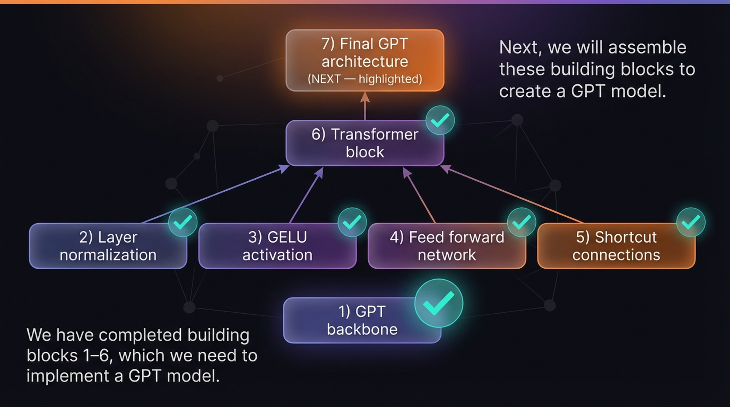
Before diving into code, let’s map out exactly what we need to build. There are 7 building blocks, and the strategy is bottom-up: implement the small pieces first, combine them into a transformer block, then stack transformer blocks into the complete model.
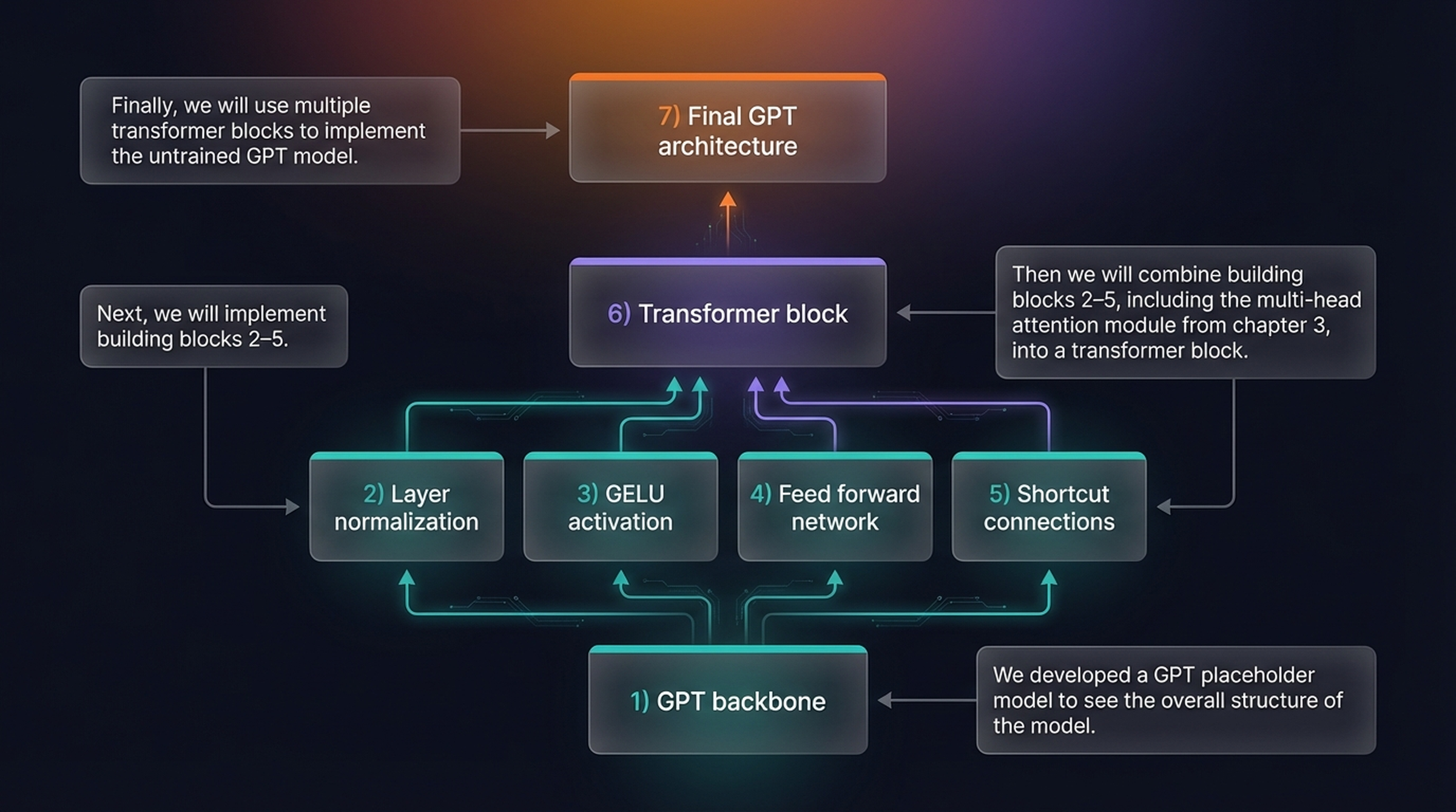
The seven building blocks of the GPT architecture, assembled bottom-up. We start with a placeholder backbone, implement components 2–5 individually, wire them into a transformer block (6), and finally assemble the complete GPT model (7).
Here’s what each block does:
1) GPT backbone — a placeholder skeleton with embeddings and an output head. Think of it as the frame of a car before you install the engine.
2) Layer normalization — stabilizes training by keeping activations centered at zero with unit variance.
3) GELU activation — a smoother alternative to ReLU that gives the optimizer more nuanced gradients to work with.
4) Feed forward network — a two-layer MLP that expands the embedding dimension by 4×, applies nonlinearity, then contracts back.
5) Shortcut connections — residual paths that bypass layers to prevent vanishing gradients in deep networks.
6) Transformer block — combines blocks 2–5 with masked multi-head attention from Chapter 3.
7) Final GPT architecture — stacks 12 transformer blocks between embedding layers and an output head.
The GPT-2 small configuration uses these exact numbers:
GPT_CONFIG_124M = {
    "vocab_size": 50257,      # Vocabulary size
    "context_length": 1024,  # Context length
    "emb_dim": 768,           # Embedding dimension
    "n_heads": 12,            # Number of attention heads
    "n_layers": 12,           # Number of layers
    "drop_rate": 0.1,         # Dropout rate
    "qkv_bias": False         # Query-Key-Value bias
}
📄 From the GPT-2 paper: The vocabulary size of 50,257 comes from GPT-2’s use of Byte Pair Encoding (BPE) operating at the byte level. Since WebText contains highly diverse internet text — code, math, Unicode, URLs, multilingual fragments — a byte-level tokenizer can encode any string without unknown tokens. The context length of 1,024 tokens was doubled from GPT-1’s 512, giving the model a much longer memory window to condition its predictions on.
Data Flow Through the GPT Model
Let’s trace exactly what happens when the sentence “Great ideas shape our” enters the model. The pipeline has several distinct stages, and understanding the shapes at each stage is crucial for debugging and building intuition.

The complete GPT I/O pipeline. Input text is tokenized into IDs (5765, 4213, 5485, 674), converted into 768-dimensional embedding vectors, processed by the GPT model, and post-processed to predict the next word: “world”.
Here’s what happens at each stage. The input text “Great ideas shape our” gets tokenized into four token IDs. Each ID is looked up in a 768-dimensional embedding table, producing four 768-dim vectors. These vectors flow through the GPT model, which returns one output vector per input token — same count in, same count out.
The critical detail: the model’s job is to make the last output vector encode enough information to predict the next word. So the output at position 4 (corresponding to “our”) contains the model’s best guess for what comes after “our” — and if the model is well-trained, that guess will be “world”.
Since each input token produces an output at the same position, the first input token (“Great”) effectively has no “previous word” to predict, which is why the output text starts from “ideas” rather than “Great”.
Layer Normalization — Stable Training Foundations
Deep neural networks have a training stability problem. As data flows through dozens of layers, activations can drift to extreme values — either exploding or vanishing. Layer normalization is the standard fix: it adjusts each layer’s outputs to have a mean of 0 and a variance of 1.
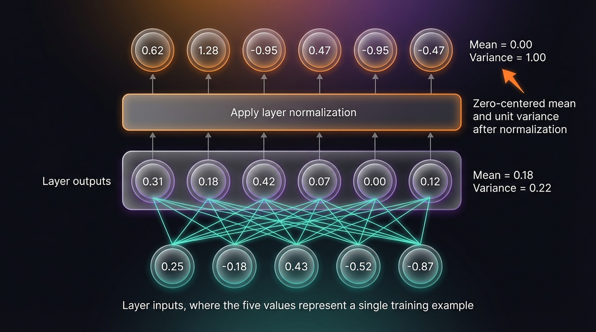
Layer normalization in action. The six layer outputs (mean = 0.18, variance = 0.22) are normalized to have mean = 0.00 and variance = 1.00. The operation subtracts the mean and divides by the standard deviation, then applies learnable scale and shift parameters.
The mechanism is straightforward: subtract the mean across the feature dimension, divide by the standard deviation, then apply two learnable parameters (scale and shift) that the model adjusts during training. Here’s the implementation:
class LayerNorm(nn.Module):
    def __init__(self, emb_dim):
        super().__init__()
        self.eps = 1e-5
        self.scale = nn.Parameter(torch.ones(emb_dim))
        self.shift = nn.Parameter(torch.zeros(emb_dim))

    def forward(self, x):
        mean = x.mean(dim=-1, keepdim=True)
        var = x.var(dim=-1, keepdim=True, unbiased=False)
        norm_x = (x - mean) / torch.sqrt(var + self.eps)
        return self.scale * norm_x + self.shift
A subtle but important implementation detail: we use unbiased=False in the variance calculation. This divides by n rather than n-1, matching the original GPT-2 implementation (which was built in TensorFlow where this is the default). For 768-dimensional embeddings, the practical difference is negligible, but matching this ensures compatibility when loading pretrained weights later.
Unlike batch normalization — which normalizes across the batch dimension — layer normalization normalizes across the feature dimension. This makes it independent of batch size, which is critical for LLMs where batch sizes can vary dramatically between training and inference.
📄 From the GPT-2 paper — Pre-LayerNorm: The original 2017 “Attention Is All You Need” transformer used Post-LayerNorm — normalization after each sublayer. GPT-2 moved layer normalization to the input of each sub-block and added an additional LayerNorm after the final self-attention block. This seemingly small change (Pre-LayerNorm vs Post-LayerNorm) has an outsized practical impact: it produces much more stable training dynamics, especially for deep models. The paper mentions it almost in passing — one sentence — but it’s one of the most consequential architectural decisions in GPT-2, and it’s now standard in virtually all modern transformer architectures.
GELU Activation — Why Not Just ReLU?
If you’ve worked with neural networks, you’ve used ReLU: it passes positive inputs through unchanged and clamps everything negative to zero. Simple, fast, and effective for many architectures. But for transformers, the sharp corner at zero creates problems.
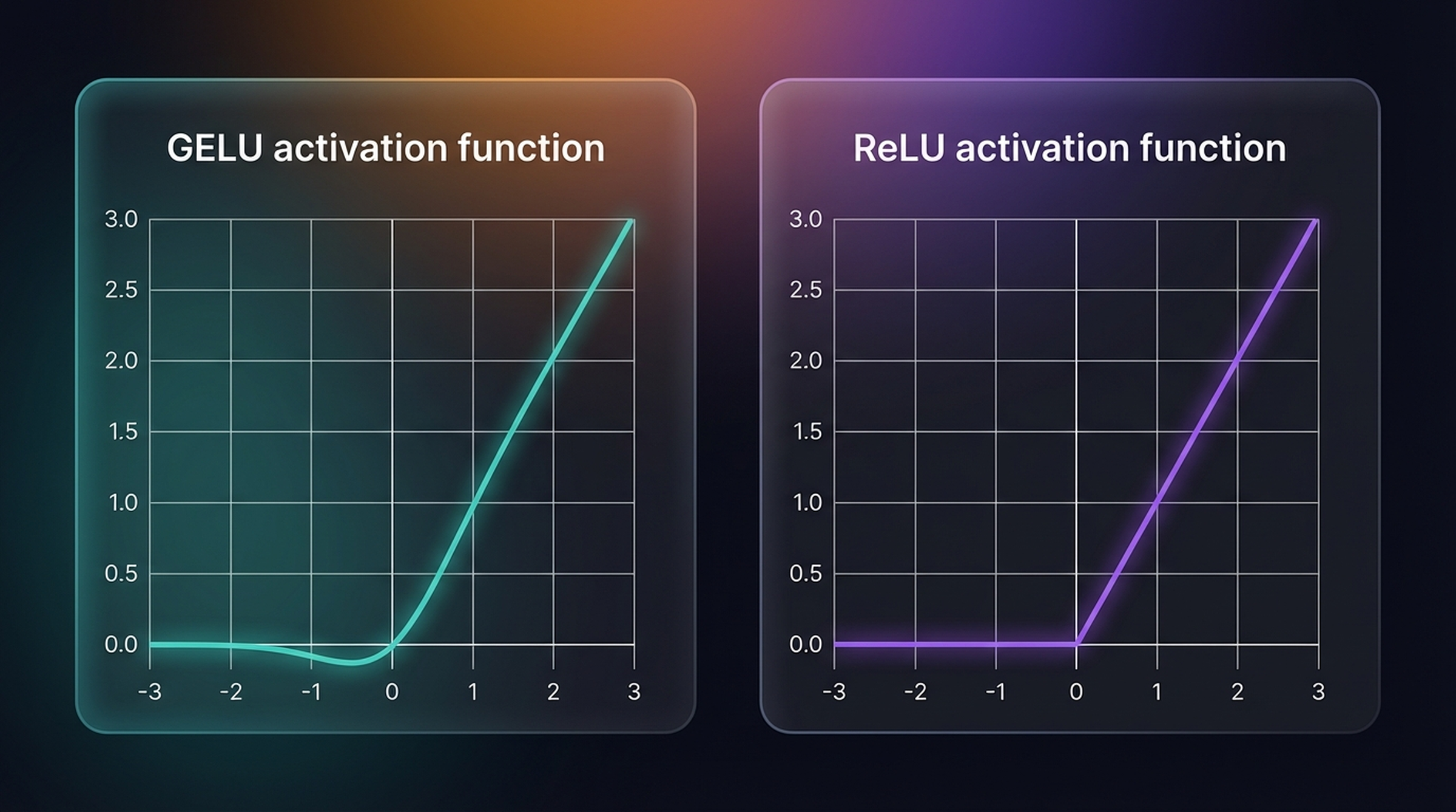
GELU (left) vs. ReLU (right). Notice how GELU is smooth everywhere — including the transition around zero — while ReLU has a hard kink at x=0. GELU also allows small non-zero outputs for slightly negative inputs.
GELU (Gaussian Error Linear Unit) is defined as x · Φ(x) where Φ is the Gaussian CDF, but in practice we use a fast tanh approximation. The key properties that make it better suited for transformers are its smoothness — giving the optimizer more nuanced gradients at every point — and the fact that slightly negative inputs can still contribute small non-zero activations rather than being silenced entirely.
class GELU(nn.Module):
    def __init__(self):
        super().__init__()

    def forward(self, x):
        return 0.5 * x * (1 + torch.tanh(
            torch.sqrt(torch.tensor(2.0 / torch.pi)) *
            (x + 0.044715 * torch.pow(x, 3))
        ))
GELU is used in GPT-2, BERT, and most modern transformer architectures. The original GPT-2 model was trained with this exact tanh approximation.
The Feed Forward Network — Expand and Contract
Every transformer block contains a small neural network called the feed forward network (FFN). Its design is elegant: take the 768-dimensional input, project it into a 4× larger space (3,072 dimensions), apply nonlinearity via GELU, then project back down to 768.

The feed forward network’s tensor shape flow. An input of shape (2, 3, 768) — batch size 2, 3 tokens, 768 embedding dimensions — is expanded to (2, 3, 3072) by the first linear layer, passed through GELU activation, and contracted back to (2, 3, 768) by the second linear layer.
Why the 4× expansion? The intuition is that the model needs more room to think. The input and output must both be 768-dimensional (so blocks can stack without dimension mismatches), but internally the network briefly visits a richer, higher-dimensional representation space where it can capture more complex patterns before compressing the result back down.
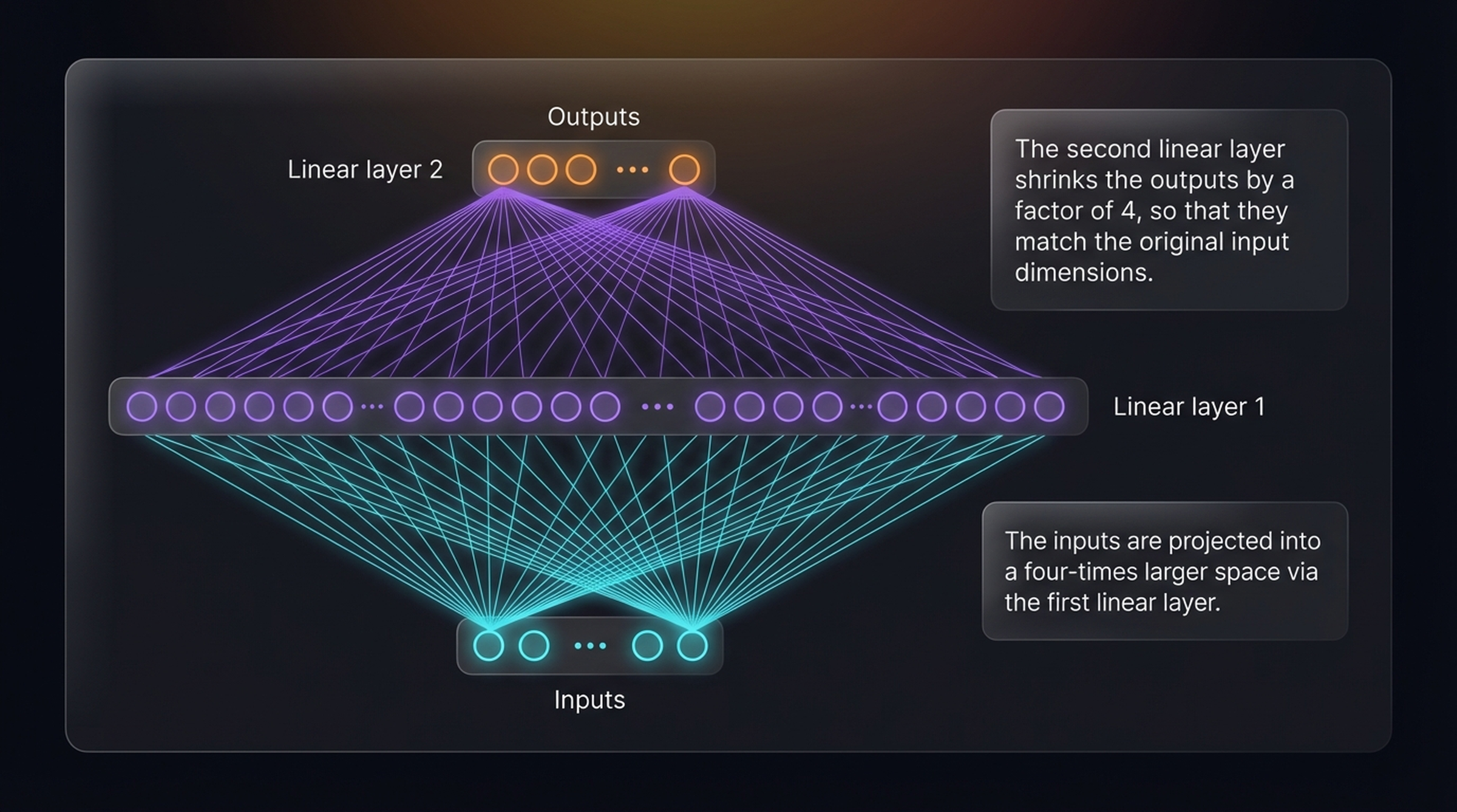
The diamond shape of the FFN visualized as a neural network diagram. Inputs at the bottom are projected into a 4× larger space via linear layer 1, then contracted back to the original dimensions via linear layer 2.
The implementation is concise:
class FeedForward(nn.Module):
    def __init__(self, cfg):
        super().__init__()
        self.layers = nn.Sequential(
            nn.Linear(cfg["emb_dim"], 4 * cfg["emb_dim"]),
            GELU(),
            nn.Linear(4 * cfg["emb_dim"], cfg["emb_dim"]),
        )

    def forward(self, x):
        return self.layers(x)
The fact that input and output dimensions are identical is not accidental — it’s what makes the modular, stackable transformer architecture possible.
Shortcut Connections — Keeping Gradients Alive
Here’s a problem that plagued deep learning for years. When you train a network with many layers, the gradients — the signals that tell each layer how to adjust its weights — shrink exponentially as they propagate backward from the output toward the input. By the time they reach the earliest layers, they’re practically zero. This is the vanishing gradient problem, and it makes deep networks nearly impossible to train.
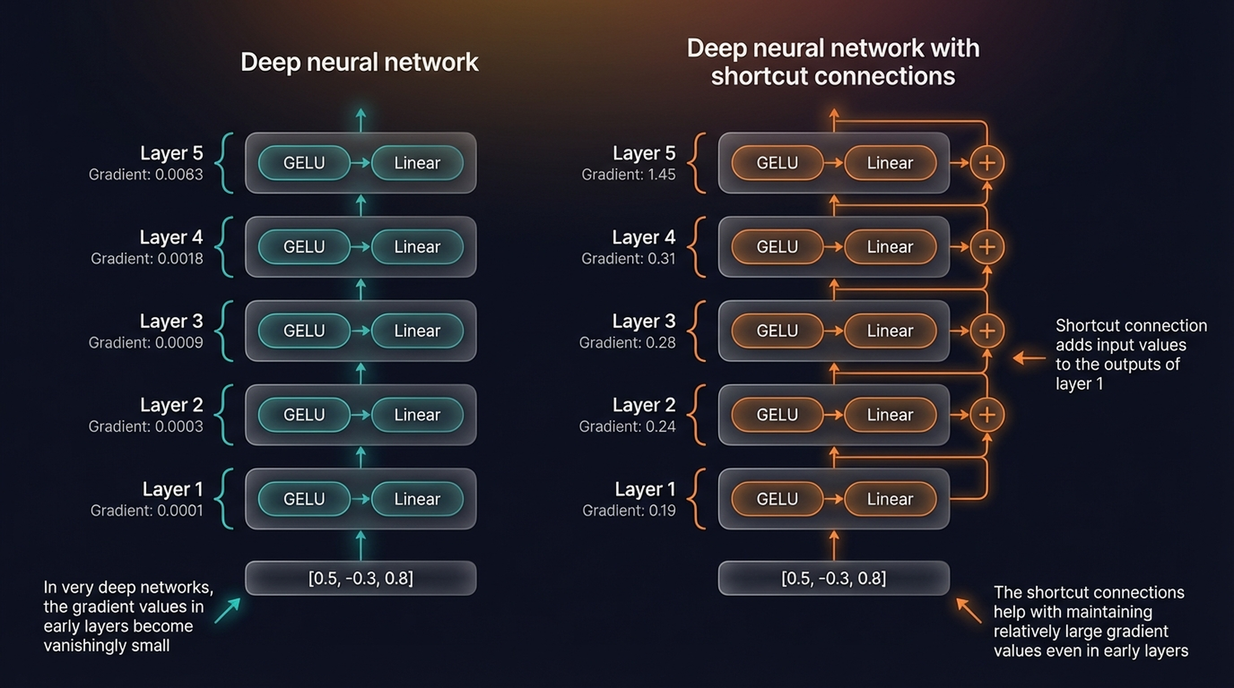
The difference is dramatic. Without shortcuts (left): gradients decay from 0.0063 at Layer 5 to 0.0001 at Layer 1 — early layers barely learn. With shortcuts (right): gradients stay healthy throughout, from 1.45 at Layer 5 to 0.19 at Layer 1.
The solution is surprisingly simple: add the input of each layer directly to its output. That’s it. In code, it’s literally x = x + layer(x). This creates an alternative, shorter path for gradients to flow through during backpropagation, bypassing the layers that would otherwise shrink them to nothing.
📄 From the GPT-2 paper — Residual weight scaling: GPT-2 introduced a modified initialization that accounts for the accumulation of signal on the residual path as model depth increases. The weights of residual layers are scaled by 1/√N at initialization, where N is the number of residual layers. Without this, each shortcut connection adds to the running sum, and by layer 48 (GPT-2 XL) the variance of activations could explode. Combined with Pre-LayerNorm, this 1/√N scaling is what allows GPT-2 to scale up to 48 transformer blocks while training smoothly.
The Transformer Block — Putting It All Together
Now we combine everything. The transformer block is the fundamental repeating unit of the GPT architecture — the one component that gets duplicated 12 times (or 48 times in GPT-2 XL) to create the full model. It wires together all the building blocks we’ve just implemented in a specific order.
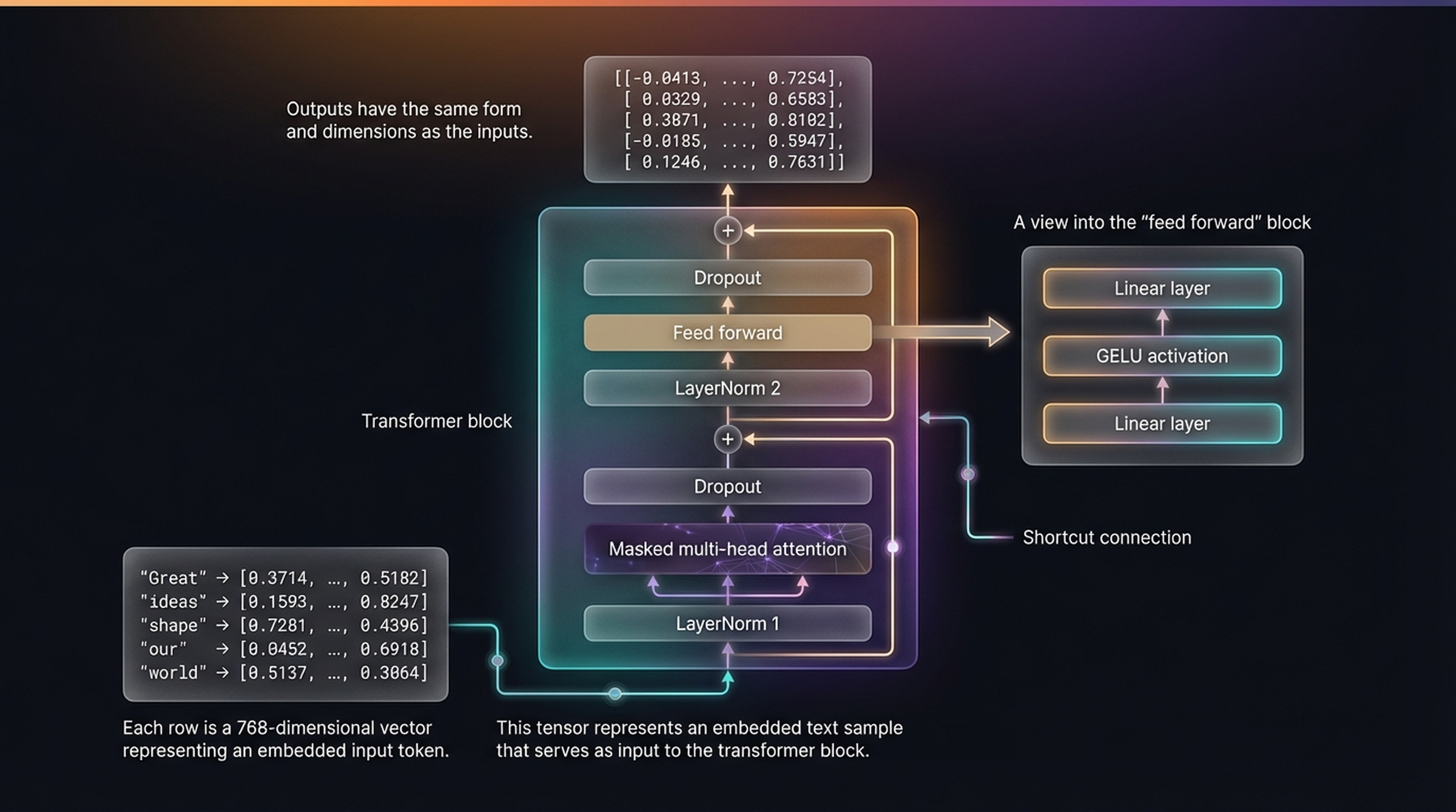
The complete transformer block. Input token embeddings flow through LayerNorm 1 → Masked multi-head attention → Dropout → Shortcut connection → LayerNorm 2 → Feed forward network → Dropout → Shortcut connection → Output.
The data flow follows two sub-blocks, each with its own shortcut connection:
Sub-block 1 (Attention): Apply LayerNorm, then masked multi-head attention, then dropout, then add the original input back (shortcut connection).
Sub-block 2 (FFN): Apply LayerNorm, then the feed forward network, then dropout, then add the sub-block 1 output back (second shortcut connection).
Notice that normalization happens before each sublayer (Pre-LayerNorm), not after. And the input and output dimensions are identical — 768 dimensions per token — which is precisely what allows these blocks to stack seamlessly.
class TransformerBlock(nn.Module):
    def __init__(self, cfg):
        super().__init__()
        self.att = MultiHeadAttention(
            d_in=cfg["emb_dim"],
            d_out=cfg["emb_dim"],
            context_length=cfg["context_length"],
            num_heads=cfg["n_heads"],
            dropout=cfg["drop_rate"],
            qkv_bias=cfg["qkv_bias"]
        )
        self.ff = FeedForward(cfg)
        self.norm1 = LayerNorm(cfg["emb_dim"])
        self.norm2 = LayerNorm(cfg["emb_dim"])
        self.drop_shortcut = nn.Dropout(cfg["drop_rate"])

    def forward(self, x):
        # Sub-block 1: Attention with shortcut
        shortcut = x
        x = self.norm1(x)
        x = self.att(x)
        x = self.drop_shortcut(x)
        x = x + shortcut

        # Sub-block 2: FFN with shortcut
        shortcut = x
        x = self.norm2(x)
        x = self.ff(x)
        x = self.drop_shortcut(x)
        x = x + shortcut
        return x
Each token’s output from the transformer block is now a context vector — it encodes information not just about that token, but about the entire input sequence via the attention mechanism. The physical dimensions haven’t changed (still 768-dim per token), but the content of each vector has been enriched with contextual information from all other tokens.
The Complete GPT-2 Architecture
All building blocks are complete — from the GPT backbone through layer normalization, GELU, feed forward networks, shortcut connections, and the transformer block. Now we assemble them into the final GPT architecture.
With every component in place, the full GPT model is surprisingly compact. Here’s the complete architecture: token embeddings + positional embeddings → dropout → 12 transformer blocks → final LayerNorm → linear output layer. That’s it.
class GPTModel(nn.Module):
    def __init__(self, cfg):
        super().__init__()
        self.tok_emb = nn.Embedding(cfg["vocab_size"], cfg["emb_dim"])
        self.pos_emb = nn.Embedding(cfg["context_length"], cfg["emb_dim"])
        self.drop_emb = nn.Dropout(cfg["drop_rate"])

        self.trf_blocks = nn.Sequential(
            *[TransformerBlock(cfg) for _ in range(cfg["n_layers"])]
        )

        self.final_norm = LayerNorm(cfg["emb_dim"])
        self.out_head = nn.Linear(
            cfg["emb_dim"], cfg["vocab_size"], bias=False
        )

    def forward(self, in_idx):
        batch_size, seq_len = in_idx.shape
        tok_embeds = self.tok_emb(in_idx)
        pos_embeds = self.pos_emb(
            torch.arange(seq_len, device=in_idx.device)
        )
        x = tok_embeds + pos_embeds
        x = self.drop_emb(x)
        x = self.trf_blocks(x)
        x = self.final_norm(x)
        logits = self.out_head(x)
        return logits
The output layer maps each token’s 768-dimensional representation to a 50,257-dimensional vector — one logit per vocabulary token. The last output row is what matters for generation: it represents the model’s prediction for the next word.
The total raw parameter count comes to about 163 million. But the original GPT-2 paper reports 124 million. The difference? Weight tying — the token embedding layer and the output layer share the same weight matrix. Since that matrix is 50,257 × 768 (roughly 38.6M parameters), removing the duplicate count gives us the reported 124M figure. At float32 precision, this model occupies about 622 MB of memory.
📄 From the GPT-2 paper — The model family: The beauty of this architecture is that the same code scales across four model sizes just by changing config numbers:
| Model | Layers | d_model | Heads | Parameters |
|---|---|---|---|---|
| Small | 12 | 768 | 12 | 124M |
| Medium | 24 | 1,024 | 16 | 345M |
| Large | 36 | 1,280 | 20 | 762M |
| XL | 48 | 1,600 | 25 | 1,542M |
GPT-2 XL has 48 transformer blocks — 4× what we implemented — but the code is identical. Only the config dict changes. GPT-3 is fundamentally the same architecture scaled up to 175 billion parameters. The architecture we built is the exact blueprint that powered the GPT revolution.
📄 Training details from the paper: GPT-2 was trained with a batch size of 512 sequences of 1,024 tokens each — so each training step processes roughly 524K tokens. The training objective is simply: predict the next token. No task labels, no supervised signal, no reward model. All downstream capabilities — question answering, translation, summarization — emerge from this single, unsupervised objective.
Generating Text — The Autoregressive Loop
We have the architecture. Now let’s make it produce text. The generation process is iterative: predict one token, append it to the context, feed the extended context back in, predict the next token, repeat. This is called autoregressive generation — each prediction depends on all previous ones.
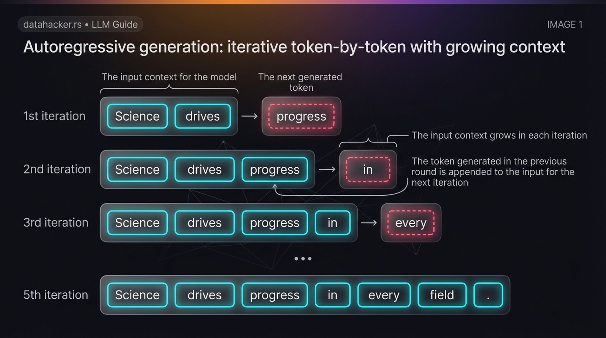
Autoregressive generation in action. Starting with “Science drives”, the model predicts “progress” (iteration 1), appends it, predicts “in” (iteration 2), appends it, predicts “every” (iteration 3), and so on. The context grows with each step until the full sentence emerges: “Science drives progress in every field.”
Each iteration follows a specific pipeline. Let’s trace through a single step:
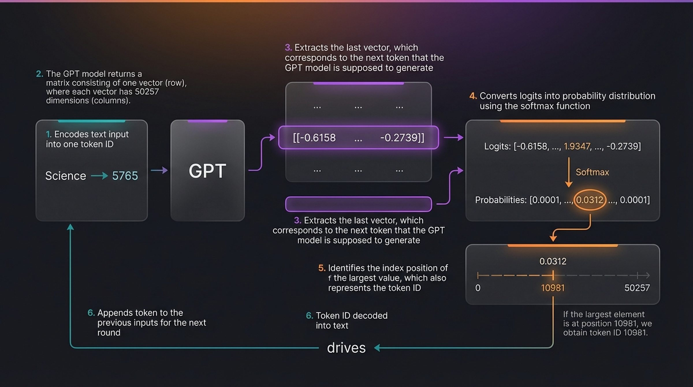
The mechanics of a single generation step. (1) Encode input to token ID, (2) GPT returns a matrix with one 50,257-dim vector per input token, (3) extract the last vector, (4) apply softmax to get probabilities, (5) argmax to find the highest-probability token ID, (6) decode back to text and append for the next round.
Here’s the generation function in PyTorch:
def generate_text_simple(model, idx, max_new_tokens, context_size):
    for _ in range(max_new_tokens):
        idx_cond = idx[:, -context_size:]     # Crop to max context
        with torch.no_grad():
            logits = model(idx_cond)

        logits = logits[:, -1, :]             # Last token's output only
        probas = torch.softmax(logits, dim=-1)
        idx_next = torch.argmax(probas, dim=-1, keepdim=True)
        idx = torch.cat((idx, idx_next), dim=1)   # Append prediction
    return idx
A technical note: the softmax step is technically redundant for greedy decoding — argmax of the raw logits gives the same result as argmax of the softmax probabilities, since softmax preserves ordering. But including it makes the probability interpretation explicit and is necessary for more advanced sampling strategies (temperature scaling, top-k, top-p) that we’ll explore in future chapters.
This process unfolds iteration by iteration, with the context growing each time:
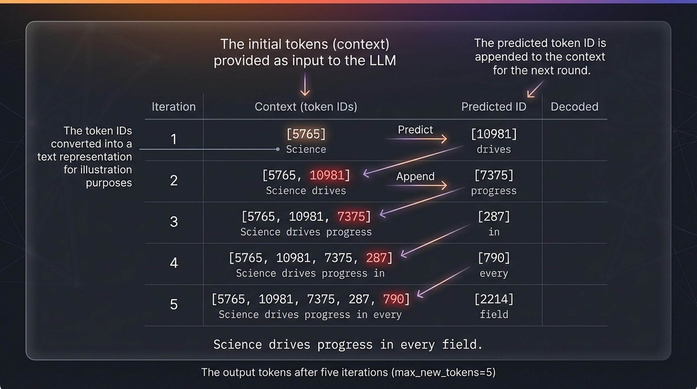
Five iterations of autoregressive generation. Starting with token ID 5765 (“Science”), each iteration predicts the next token ID, appends it to the context, and feeds the expanded context back into the model. After five iterations: “Science drives progress in every field.”
What We Built
Let’s take stock. In this chapter, we implemented a complete GPT-2 model from scratch — every layer, every connection, every normalization. The key architectural insights worth remembering:
Layer normalization and shortcut connections are what make deep training possible. Without them, gradients vanish and 12+ layer models simply don’t converge.
The 4× FFN expansion provides the model with representational capacity — a brief excursion into a richer space where it can capture more complex patterns.
Repeated, identical transformer blocks create depth without complexity. The same code, the same architecture, duplicated 12 or 48 times.
Autoregressive generation is elegant in its simplicity: predict, append, repeat.
The model is structurally complete, but right now it produces gibberish — random outputs from random weights. That’s expected. The architecture is the skeleton; training brings it to life. In the next chapter, we implement the training loop and pretrain the model to actually generate coherent text.
📄 The scaling story — why this matters: Perhaps the most striking finding from the GPT-2 paper: even GPT-2 XL (1.5B parameters) still underfits WebText. Performance improved log-linearly with model size, with no sign of plateau. This observation became the foundation of the scaling laws hypothesis — the idea that you can predictably improve performance by scaling up parameters, data, and compute. It directly motivated GPT-3 (175B) and eventually GPT-4. The architecture didn’t change. The scale did. What we built today is the seed.
📚 References & Further Reading:
- Radford, A. et al. (2019). “Language Models are Unsupervised Multitask Learners.” OpenAI.
- Vaswani, A. et al. (2017). “Attention Is All You Need.” NeurIPS.
- He, K. et al. (2016). “Deep Residual Learning for Image Recognition.” CVPR.
- Hendrycks, D. & Gimpel, K. (2016). “Gaussian Error Linear Units (GELUs).” arXiv.
- Ba, J.L. et al. (2016). “Layer Normalization.” arXiv.
- Raschka, S. (2024). Build a Large Language Model (From Scratch). Manning Publications.
Written by VLADIMIR MATIĆ, PhD ·