LLM_log #004 From Scratch: Working with Text Data — Embeddings for LLMs
Highlights: Before we can build or train a Large Language Model, we need to solve a fundamental problem — LLMs cannot process raw text. In today’s post, we’ll walk through the complete pipeline that converts human-readable text into numerical vectors that a neural network can work with. We’ll cover tokenization, vocabulary building, byte pair encoding, sliding window sampling, and how token and positional embeddings come together to form the final input to a GPT-like transformer. So let’s begin!
Source: This post is based on Chapter 2 of Sebastian Raschka’s Build a Large Language Model (From Scratch). The goal is to present the most important ideas along with clear visuals, and it can be used for a quick recap of the main concepts.
The Big Picture — Three Stages to a Working LLM
Building a language model from scratch is a three-stage journey. First we construct the architecture — tokenizer, attention mechanism, and transformer blocks. Then we pretrain it on billions of tokens using next-token prediction. Finally, we specialize the base model into a classifier or chat assistant through fine-tuning.
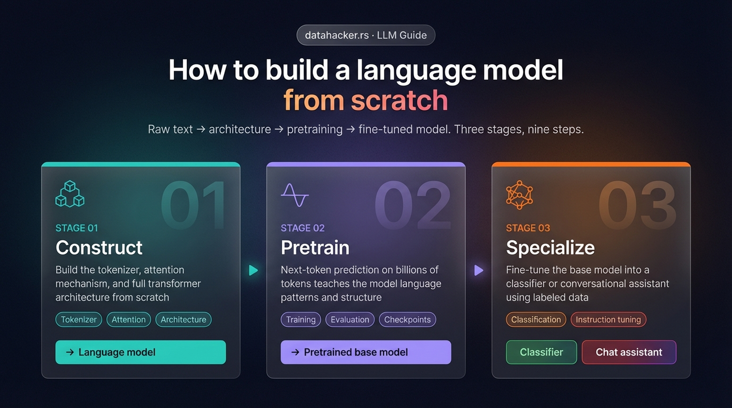
The high-level roadmap: three stages take us from raw text to a specialized model. Stage 01 builds the core architecture, Stage 02 trains it on massive text data, and Stage 03 adapts it for specific tasks like classification or conversation.
This post focuses on the very first part of Stage 01 — specifically, how raw text gets transformed into the numerical input that the transformer architecture can process. Here is a more detailed view of all nine steps across the three stages:
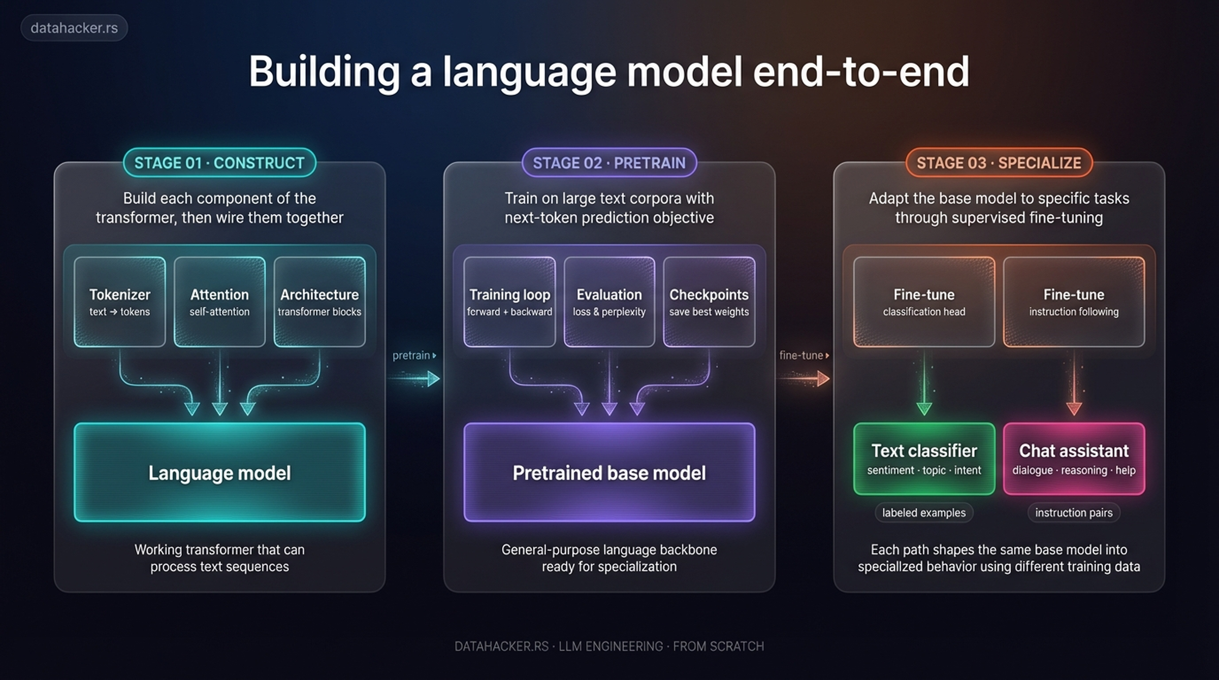
The detailed end-to-end pipeline. Each stage breaks down into concrete steps: Construct covers the tokenizer, attention, and architecture; Pretrain handles the training loop, evaluation, and checkpoints; Specialize branches into classification or instruction-tuned chat. Today we zoom into the earliest steps — tokenization through embeddings.
Why Embeddings? — LLMs Can’t Read
Deep neural networks, including LLMs, cannot process raw text directly. Text is categorical — the word “cat” has no inherent numerical meaning that a neural network can multiply or add. To make text compatible with the mathematical operations inside a neural network, we need to represent words as continuous-valued vectors. This process is called embedding.
The core idea: we build a mapping from discrete objects (words, images, audio clips) to points in a continuous vector space. Different data types need different embedding models — a text embedding model won’t work for audio — but the output is always the same: a dense numerical vector.
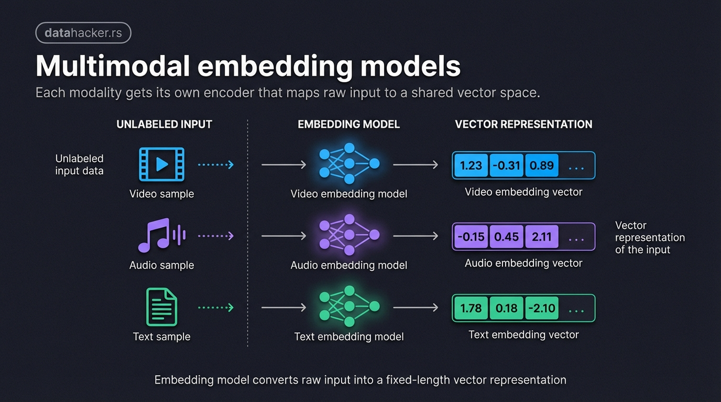
Embedding models convert raw input data — video, audio, text — into dense vector representations. Each modality requires its own specialized model, but the result is always a numerical vector that neural networks can process. Here we show 3-dimensional vectors for simplicity; in practice, GPT-2 uses 768 dimensions and GPT-3 uses up to 12,288.
Word Embeddings — Similar Meanings, Nearby Vectors
One of the earliest breakthroughs in word embeddings was Word2Vec. The insight: words that appear in similar contexts tend to have similar meanings. By training a neural network to predict context words from a target word, we get vector representations where semantic relationships are preserved geometrically.
When we project these vectors to 2D, the structure becomes visible — animals cluster near animals, cities appear near their countries, and degree words (long → longer → longest) line up along a shared axis.
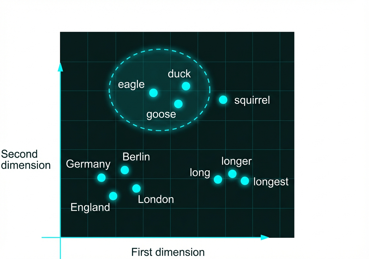
2D projection of word embeddings trained with Word2Vec. Semantically similar words cluster together: animal types group near each other, cities appear near their countries, and degree words align along a dimension. The vector for “squirrel” sits near the bird cluster — semantically related animals cluster together in embedding space.
However, modern LLMs don’t use pre-trained Word2Vec. Instead, they learn their own embeddings as part of training — the embedding layer is optimized end-to-end together with the rest of the model. This means embeddings are tailored to the specific task. GPT-2 (smallest) uses 768-dimensional embeddings; GPT-3 (175B) uses 12,288 dimensions.
The Complete Pipeline — Text to Transformer Input
Before we dig into each step, here is the full picture. Every piece of text entering a GPT-like model passes through this pipeline:
Raw text → Tokenize → Token IDs → Token embeddings + Positional embeddings → Input embeddings → Transformer
We’ll use a running example throughout this post to keep things concrete. Our input sentence is:
“AI models learn from data.”
This sentence will appear in every figure below, going through each transformation step, so you can trace it end to end.
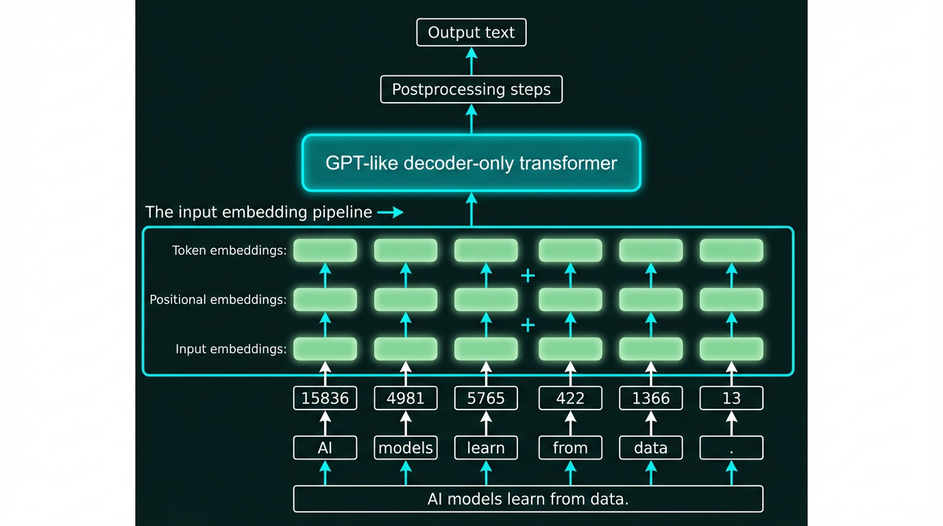
The complete input embedding pipeline. Our example sentence “AI models learn from data.” is tokenized into six tokens, mapped to token IDs [15836, 4981, 5765, 422, 1366, 13], looked up as embedding vectors, combined with positional embeddings, and fed into the GPT-like transformer. We’ll build this pipeline step by step in the sections that follow.
Step 1: Tokenization — Breaking Text Into Pieces
The first step in any LLM pipeline is tokenization — splitting raw text into individual units called tokens. In the simplest case, tokens are words and punctuation marks.
Let’s see how our running example gets tokenized:
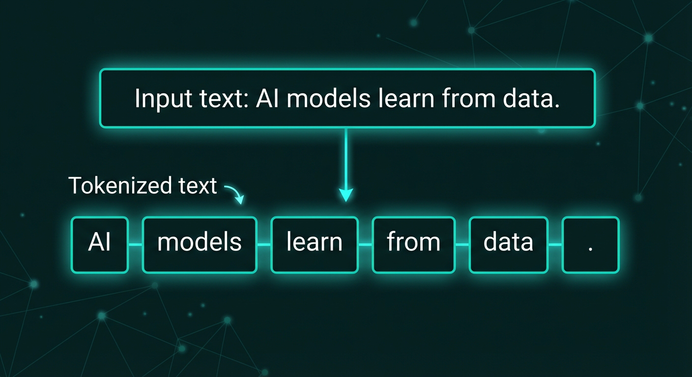
Tokenization splits “AI models learn from data.” into six tokens: [“AI”, “models”, “learn”, “from”, “data”, “.”] — each word becomes a separate token, and punctuation like the period is also treated as its own token.
Notice that:
– Each word becomes a separate token
– The period is separated as its own token
– Whitespace is used to split but isn’t kept
– This gives us exactly 6 tokens for our example sentence
This simple whitespace-and-punctuation splitting is a reasonable starting point, but modern LLMs use more sophisticated methods (like Byte Pair Encoding) that we’ll cover shortly.
Building a Simple Tokenizer in Python
Let’s implement a basic tokenizer class that handles this process. Here’s a clean implementation:
import re

class SimpleTokenizer:
    def __init__(self, vocab):
        """Initialize tokenizer with vocabulary dictionary"""
        self.token_to_id = vocab
        self.id_to_token = {idx: token for token, idx in vocab.items()}

    def encode(self, text):
        """Convert text to list of token IDs"""
        # Split on whitespace and punctuation
        tokens = re.findall(r'\w+|[^\w\s]', text)
        # Map tokens to IDs
        ids = [self.token_to_id.get(token, self.token_to_id['<UNK>'])
               for token in tokens]
        return ids

    def decode(self, ids):
        """Convert list of token IDs back to text"""
        tokens = [self.id_to_token[idx] for idx in ids]
        # Join with spaces, but handle punctuation
        text = ' '.join(tokens)
        text = re.sub(r'\s+([.,!?;:])', r'\1', text)
        return text

# Example usage with our sentence
vocab = {
    "AI": 15836,
    "models": 4981,
    "learn": 5765,
    "from": 422,
    "data": 1366,
    ".": 13,
    "<UNK>": 0  # Unknown token
}

tokenizer = SimpleTokenizer(vocab)
text = "AI models learn from data."
ids = tokenizer.encode(text)
print(f"Text: {text}")
print(f"IDs: {ids}")  # [15836, 4981, 5765, 422, 1366, 13]

# Decode back
reconstructed = tokenizer.decode(ids)
print(f"Reconstructed: {reconstructed}")  # "AI models learn from data."
The key components:
– encode(): Splits text → tokens → IDs
– decode(): Maps IDs → tokens → text
– Unknown token handling: Maps unseen words to <UNK> ID
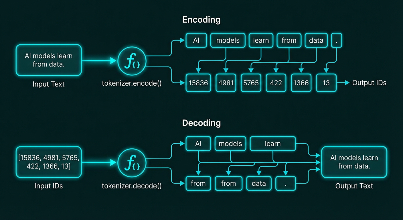
The tokenizer’s encode() method converts text to IDs, while decode() reverses the process. Our example “AI models learn from data.” encodes to [15836, 4981, 5765, 422, 1366, 13] and decodes back to the original text.
Step 2: Building a Vocabulary
Once we’ve tokenized the text, we need to map each unique token to a unique integer ID. This creates a vocabulary — a lookup table that converts tokens to numbers.
Here’s how it works:
Step 1: Tokenize the training data
If our training set is just one sentence:
"The quick brown fox jumps over the lazy dog"
We tokenize it:
["The", "quick", "brown", "fox", "jumps", "over", "the", "lazy", "dog"]
Step 2: Collect unique tokens and sort alphabetically
brown → 0
dog → 1
fox → 2
jumps → 3
lazy → 4
over → 5
quick → 6
the → 7
Note: “The” and “the” would be different tokens (case-sensitive), but for simplicity we’re showing lowercase here.
Step 3: Map tokens to IDs
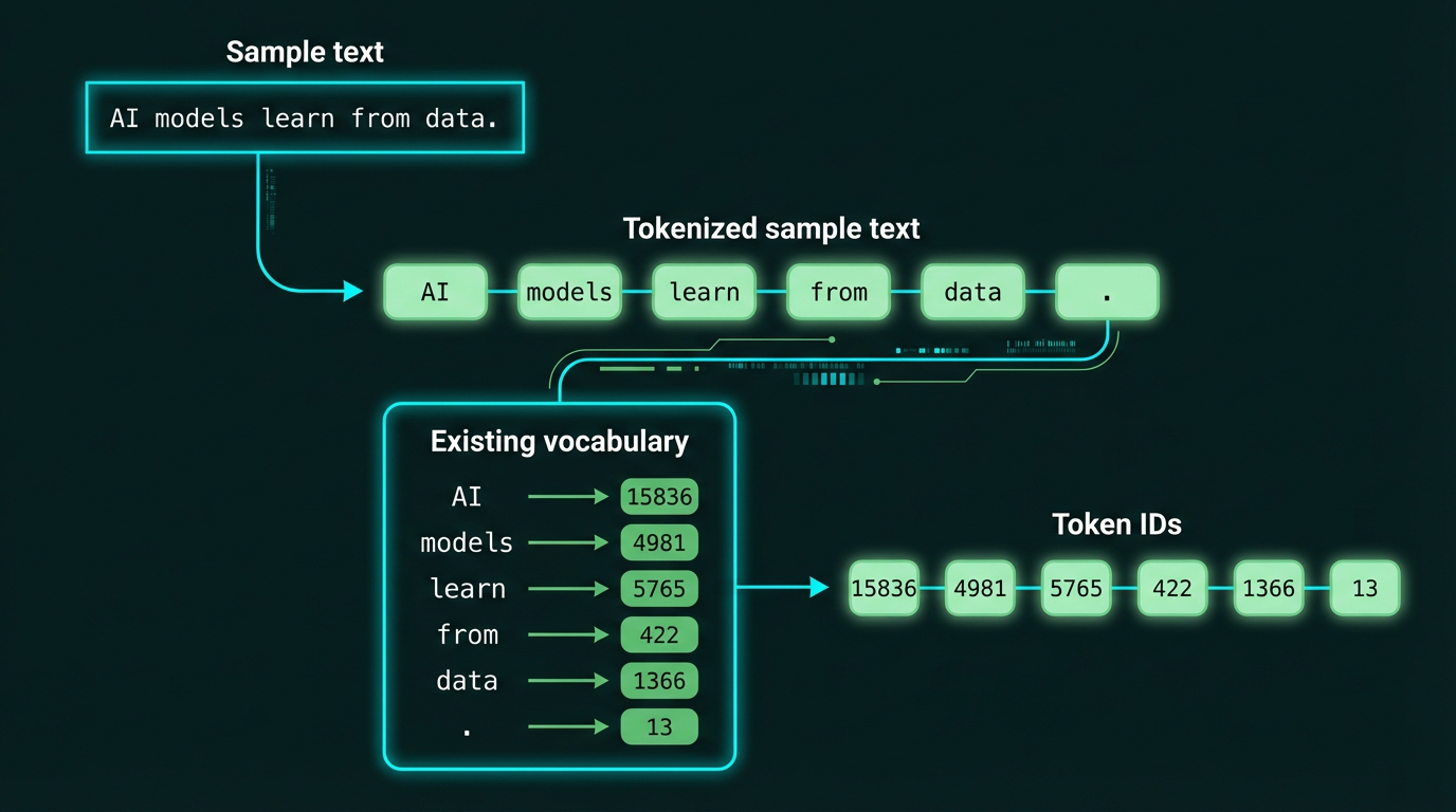
For our running example, here’s the complete tokenization and vocabulary flow:
Complete flow from sample text to token IDs. The text “AI models learn from data.” is first tokenized into individual tokens, then each token is looked up in the vocabulary to get its corresponding ID.
The vocabulary mapping for our 6 tokens:
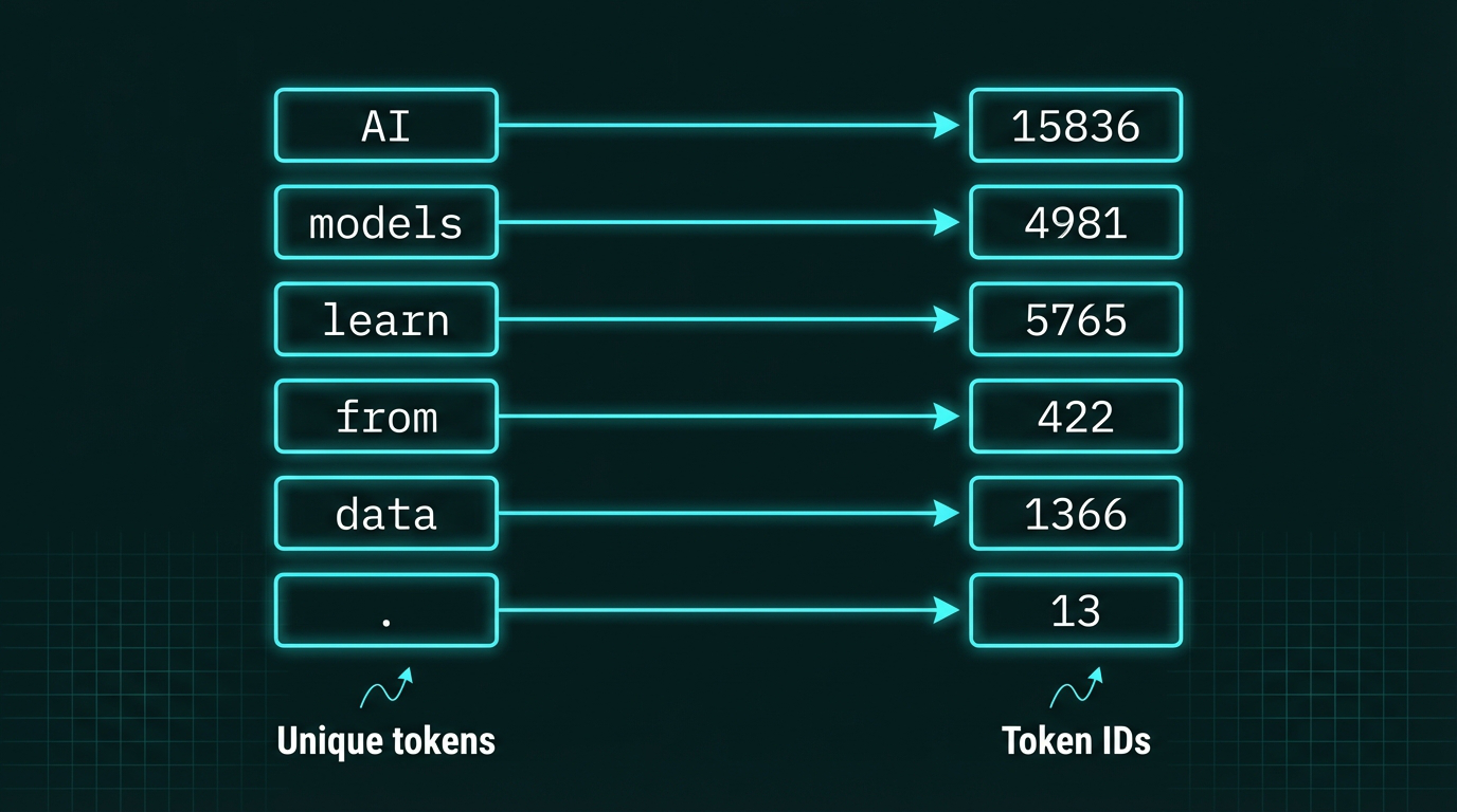
Each unique token in our vocabulary gets mapped to a unique integer ID. Here we see our six tokens from “AI models learn from data.” mapped to their corresponding IDs: AI→15836, models→4981, learn→5765, from→422, data→1366, .→13
This creates a numerical representation that neural networks can process. The vocabulary size is a key hyperparameter:
– GPT-2: 50,257 tokens
– GPT-3: 50,257 tokens (same tokenizer)
– Larger vocabularies can represent more concepts but require more parameters in the embedding layer
Step 3: Byte Pair Encoding (BPE) — Smarter Tokenization
Simple word-based tokenization has problems:
- Unknown words: If “elephant” appears in test data but not in training, we can’t map it to an ID
- Huge vocabularies: English has hundreds of thousands of words — we’d need a massive vocabulary
Byte Pair Encoding (BPE) solves this by breaking words into subword units. Instead of treating “elephant” as one token, BPE might split it into:
["ele", "phant"]
or even:
["el", "e", "ph", "ant"]
The key insight: by using subword pieces, we can represent any word (even rare ones) as a combination of common subword units.
How BPE Works
BPE starts with individual characters and iteratively merges the most frequent pairs:
- Start: Each character is a token:
['h', 'e', 'l', 'l', 'o'] - Merge most common pair: If “l” + “l” appears often, merge it:
['h', 'e', 'll', 'o'] - Repeat: Keep merging until you’ve built a vocabulary of your target size (e.g., 50,000 tokens)
GPT-2 and GPT-3 use BPE with a vocabulary of 50,257 tokens, which includes:
– Individual bytes (for any Unicode character)
– Common subwords (“ing”, “tion”, “pre”)
– Frequent whole words (“the”, “and”, “is”)
This means GPT can tokenize any text in any language without unknown tokens.
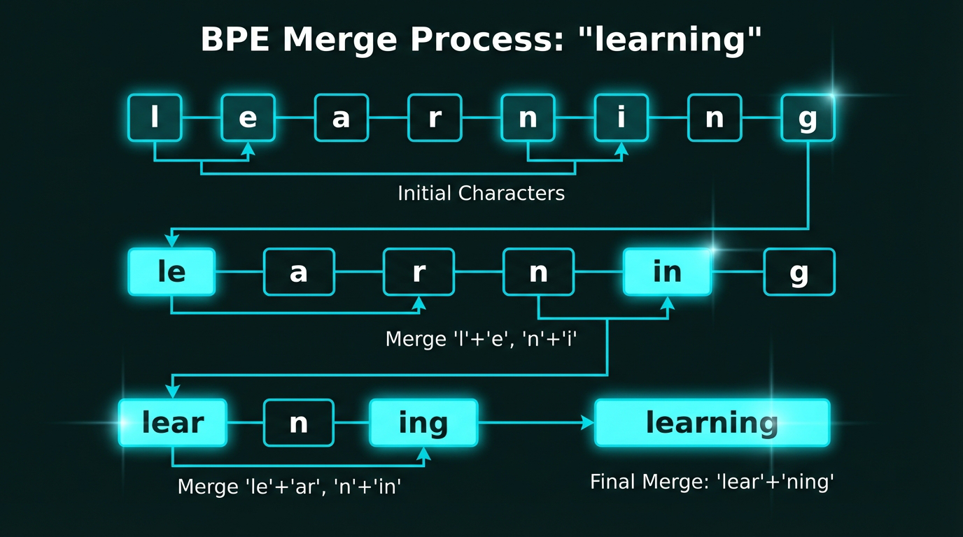
BPE progressively merges the most frequent character pairs. Starting with individual characters of “learning” → [‘l’,’e’,’a’,’r’,’n’,’i’,’n’,’g’], we merge frequent pairs like ‘l’+’e’ → ‘le’, then ‘le’+’ar’ → ‘lear’, until we have larger subword units.
Implementing BPE from Scratch
Here’s a simplified BPE implementation to understand the core algorithm:
from collections import Counter
import re

class BytePairEncoder:
    def __init__(self, vocab_size=50):
        self.vocab_size = vocab_size
        self.merges = {}  # Stores merge operations
        self.vocab = {}   # Final vocabulary

    def get_pairs(self, tokens):
        """Get all adjacent token pairs"""
        pairs = []
        for i in range(len(tokens) - 1):
            pairs.append((tokens[i], tokens[i+1]))
        return pairs

    def merge_pair(self, tokens, pair):
        """Merge all occurrences of a pair in token list"""
        new_tokens = []
        i = 0
        while i < len(tokens):
            if i < len(tokens) - 1 and (tokens[i], tokens[i+1]) == pair:
                # Merge the pair
                new_tokens.append(tokens[i] + tokens[i+1])
                i += 2
            else:
                new_tokens.append(tokens[i])
                i += 1
        return new_tokens

    def train(self, texts):
        """Learn BPE merges from training data"""
        # Start with character-level tokens
        all_tokens = []
        for text in texts:
            tokens = list(text)  # Split into characters
            all_tokens.extend(tokens)

        # Iteratively merge most frequent pairs
        for _ in range(self.vocab_size):
            pairs = []
            for text in texts:
                tokens = list(text)
                # Apply existing merges
                for merge_pair in self.merges:
                    tokens = self.merge_pair(tokens, merge_pair)
                pairs.extend(self.get_pairs(tokens))

            if not pairs:
                break

            # Find most frequent pair
            pair_counts = Counter(pairs)
            best_pair = pair_counts.most_common(1)[0][0]
            self.merges[best_pair] = len(self.merges)

        print(f"Learned {len(self.merges)} merge operations")
        return self.merges

# Example usage
bpe = BytePairEncoder(vocab_size=10)
training_texts = [
    "learning to learn",
    "machine learning",
    "deep learning"
]
merges = bpe.train(training_texts)

# The algorithm discovers merges like:
# ('l', 'e') → 'le'
# ('a', 'r') → 'ar'
# ('le', 'ar') → 'lear'
# ('n', 'i') → 'ni'
# ('ni', 'ng') → 'ning'
How it works:
1. Start with characters: “learning” → [‘l’, ‘e’, ‘a’, ‘r’, ‘n’, ‘i’, ‘n’, ‘g’]
2. Count pair frequencies: Which pairs appear most? (‘n’, ‘i’) appears twice
3. Merge most frequent: [‘l’, ‘e’, ‘a’, ‘r’, ‘ni’, ‘ng’]
4. Repeat: Keep merging until we have desired vocabulary size
GPT-2’s BPE vocab (50,257 tokens) includes:
– 256 individual bytes (handles any Unicode)
– ~40,000 common subwords
– ~10,000 frequent whole words
Step 4: Creating Training Data — Sliding Windows
LLMs are trained to predict the next token given previous context. To create training examples, we use a sliding window approach.
Given our running example:
"AI models learn from data."
Tokenized with IDs:
[15836, 4981, 5765, 422, 1366, 13]
We create input-target pairs using a sliding window:
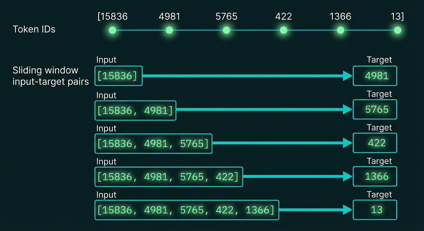
Sliding window approach for creating training data. Starting with the tokenized sequence [15836, 4981, 5765, 422, 1366, 13], we create multiple input-target pairs where each input is a growing prefix and the target is the next token. This teaches the model to predict what comes next.
Each training step:
1. Takes a sequence of token IDs as input
2. Predicts the next token ID
3. Compares prediction to actual next token
4. Updates model weights to improve prediction
This is called autoregressive training — the model learns to generate text one token at a time.
Implementing a DataLoader for LLM Training
In practice, we need to efficiently generate these input-target pairs for training. Here’s a PyTorch-style DataLoader:
import torch
from torch.utils.data import Dataset, DataLoader

class LLMDataset(Dataset):
    def __init__(self, token_ids, context_length=4, stride=1):
        """
        Args:
            token_ids: List of token IDs for entire dataset
            context_length: Maximum sequence length (context window)
            stride: Step size for sliding window (1 = every position)
        """
        self.token_ids = token_ids
        self.context_length = context_length
        self.stride = stride

    def __len__(self):
        # Number of possible sequences
        return (len(self.token_ids) - self.context_length) // self.stride

    def __getitem__(self, idx):
        # Get sequence starting at position idx * stride
        start_idx = idx * self.stride
        end_idx = start_idx + self.context_length

        # Input: tokens[start:end]
        input_seq = self.token_ids[start_idx:end_idx]
        # Target: tokens[start+1:end+1] (shifted by 1)
        target_seq = self.token_ids[start_idx + 1:end_idx + 1]

        return (
            torch.tensor(input_seq, dtype=torch.long),
            torch.tensor(target_seq, dtype=torch.long)
        )

# Example with our token sequence
token_ids = [15836, 4981, 5765, 422, 1366, 13]  # "AI models learn from data."

dataset = LLMDataset(token_ids, context_length=4, stride=1)
dataloader = DataLoader(dataset, batch_size=2, shuffle=False)

print(f"Dataset has {len(dataset)} sequences")

for batch_idx, (inputs, targets) in enumerate(dataloader):
    print(f"\nBatch {batch_idx}:")
    print(f"  Inputs:  {inputs}")
    print(f"  Targets: {targets}")

# Output:
# Dataset has 2 sequences
#
# Batch 0:
#   Inputs:  tensor([[15836, 4981, 5765,   422],
#                    [ 4981, 5765,   422,  1366]])
#   Targets: tensor([[ 4981, 5765,   422,  1366],
#                    [ 5765,   422,  1366,    13]])
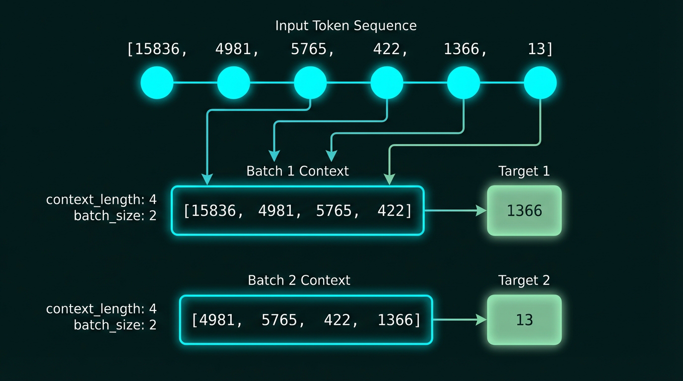
Creating training batches with sliding windows. From our token sequence, we extract overlapping chunks of length 4, creating input-target pairs. Multiple sequences are batched together for efficient GPU training.
Key parameters:
– context_length: How many tokens the model sees at once (GPT-3 uses 2048)
– stride: How much to shift the window (1 = maximum overlap)
– batch_size: How many sequences to process in parallel (typically 32-512)
Step 5: Token Embeddings — From IDs to Vectors
Token IDs are still just discrete integers. To feed them into a neural network, we need continuous vectors.
The embedding layer is surprisingly simple — it’s just a lookup table:
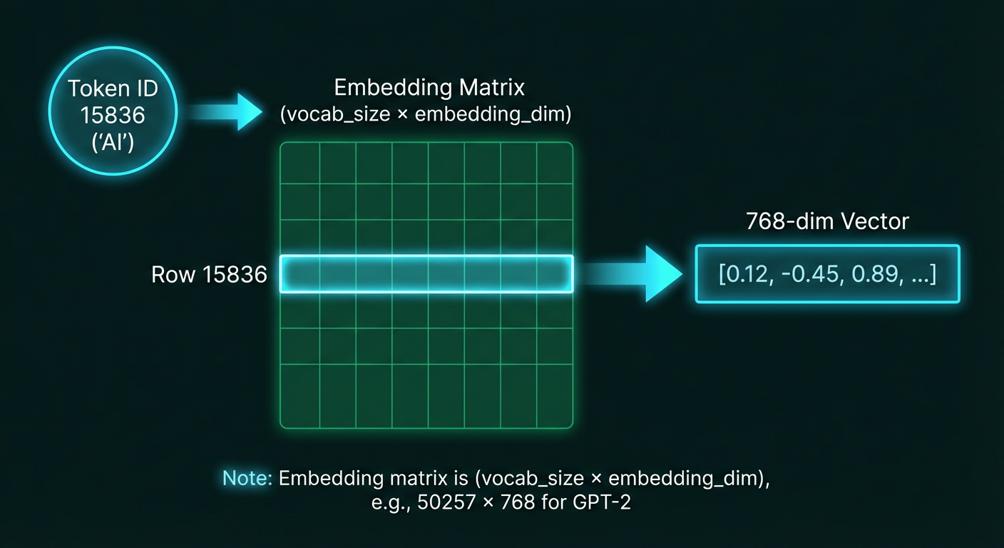
Token embedding as matrix lookup. The embedding matrix has one row per vocabulary token (50,257 rows for GPT-2) and 768 columns (embedding dimensions). When we input token ID 15836 (“AI”), we simply retrieve row 15836 to get the 768-dimensional embedding vector.
When you input token ID 15836 (which represents “AI”), you simply look up row 15836 in this matrix and get its 768-dimensional vector.
For our example sentence with IDs [15836, 4981, 5765, 422, 1366, 13]:
15836 → [0.12, -0.45, ...]  (768 dims)
4981  → [-0.33, 0.71, ...]  (768 dims)
5765  → [0.88, -0.11, ...]  (768 dims)
422   → [0.45, 0.92, ...]   (768 dims)
1366  → [-0.67, 0.34, ...]  (768 dims)
13    → [0.21, -0.88, ...]  (768 dims)
Now we have a sequence of 6 embedding vectors, each 768-dimensional.
These embeddings are learned during training — the model updates them to encode semantic meaning.
Implementing the Embedding Layer
In PyTorch, the embedding layer is remarkably simple:
import torch
import torch.nn as nn

class TokenEmbedding(nn.Module):
    def __init__(self, vocab_size, embedding_dim):
        """
        Args:
            vocab_size: Number of unique tokens (50257 for GPT-2)
            embedding_dim: Size of embedding vectors (768 for GPT-2)
        """
        super().__init__()
        # This is just a learnable lookup table
        self.embedding = nn.Embedding(vocab_size, embedding_dim)

    def forward(self, token_ids):
        """
        Args:
            token_ids: Tensor of shape (batch_size, seq_length)
        Returns:
            embeddings: Tensor of shape (batch_size, seq_length, embedding_dim)
        """
        return self.embedding(token_ids)

# Create embedding layer for GPT-2 size
vocab_size = 50257
embedding_dim = 768
token_emb = TokenEmbedding(vocab_size, embedding_dim)

# Embed our example sentence
token_ids = torch.tensor([[15836, 4981, 5765, 422, 1366, 13]])  # Shape: (1, 6)
embeddings = token_emb(token_ids)  # Shape: (1, 6, 768)

print(f"Input shape: {token_ids.shape}")
print(f"Output shape: {embeddings.shape}")
print(f"First token (ID 15836 = 'AI') embedding:")
print(embeddings[0, 0, :10])  # Show first 10 dimensions

# Output:
# Input shape: torch.Size([1, 6])
# Output shape: torch.Size([1, 6, 768])
# First token (ID 15836 = 'AI') embedding:
# tensor([-0.0234,  0.0123, -0.0445,  0.0891, -0.0567,  0.0234,
#         -0.0123,  0.0789, -0.0345,  0.0156], grad_fn=...)
Under the hood:
# What nn.Embedding actually does:
# 1. Creates a weight matrix of shape (vocab_size, embedding_dim)
# 2. For each token ID, retrieves the corresponding row

# Equivalent manual implementation:
class ManualEmbedding:
    def __init__(self, vocab_size, embedding_dim):
        # Initialize random embedding matrix
        self.weight = torch.randn(vocab_size, embedding_dim) * 0.01

    def forward(self, token_ids):
        # Simple matrix indexing
        return self.weight[token_ids]

# These are equivalent:
# embeddings = embedding_layer(token_ids)
# embeddings = embedding_layer.weight[token_ids]
Memory requirements:
– GPT-2 (117M params): 50,257 × 768 = 38.6 million embedding parameters
– GPT-3 (175B params): 50,257 × 12,288 = 617.6 million embedding parameters
– This is just the embedding layer — the transformer layers have many more parameters!
Step 6: Positional Embeddings — Encoding Word Order
Token embeddings capture what each word means, but not where it appears in the sentence.
Consider:
– “The cat chased the dog”
– “The dog chased the cat”
These have the same tokens but opposite meanings. We need to encode position.
Positional embeddings are added to token embeddings:
final_embedding = token_embedding + positional_embedding
For position 0 (first token):
pos_0 = [0.01, 0.02, 0.03, ...]
For position 1 (second token):
pos_1 = [0.02, 0.04, 0.06, ...]
These positional embeddings are also learned during training (in GPT-2/GPT-3) or use fixed sinusoidal patterns (in original Transformer).
After adding positional info, our 6 tokens become:
Token 0: [0.12, -0.45, ...] + [0.01, 0.02, ...] = [0.13, -0.43, ...]
Token 1: [-0.33, 0.71, ...] + [0.02, 0.04, ...] = [-0.31, 0.75, ...]
...
Now the transformer knows both what each word is and where it appears.
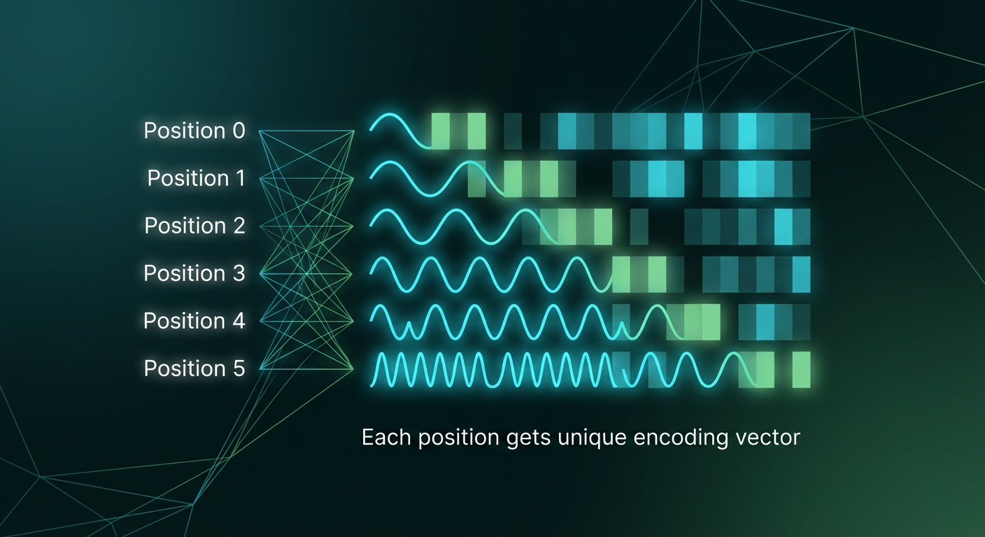
Positional encodings for the 6 positions in our example. Each position gets a unique vector that encodes its location in the sequence. These are added to token embeddings before feeding into the transformer.
Two Approaches to Positional Encoding
Approach 1: Learned Positional Embeddings (used by GPT-2/GPT-3)
class LearnedPositionalEmbedding(nn.Module):
    def __init__(self, max_len, embedding_dim):
        """
        Args:
            max_len: Maximum sequence length (2048 for GPT-3)
            embedding_dim: Same as token embedding dimension
        """
        super().__init__()
        # Another embedding layer, but for positions instead of tokens
        self.pos_embedding = nn.Embedding(max_len, embedding_dim)

    def forward(self, token_embeddings):
        batch_size, seq_len, embedding_dim = token_embeddings.shape

        # Create position indices [0, 1, 2, ..., seq_len-1]
        positions = torch.arange(seq_len, device=token_embeddings.device)
        positions = positions.unsqueeze(0).expand(batch_size, -1)

        # Look up positional embeddings
        pos_emb = self.pos_embedding(positions)

        # Add to token embeddings
        return token_embeddings + pos_emb

# Usage
max_len = 2048
embedding_dim = 768
pos_encoder = LearnedPositionalEmbedding(max_len, embedding_dim)

# Our token embeddings from before
# token_emb shape: (1, 6, 768)
final_emb = pos_encoder(embeddings)
print(f"Final embeddings shape: {final_emb.shape}")  # (1, 6, 768)
Approach 2: Sinusoidal Positional Encoding (used by original Transformer)
import math

def create_sinusoidal_embeddings(max_len, embedding_dim):
    """
    Creates fixed sinusoidal position encodings
    Different frequencies for each dimension
    """
    positions = torch.arange(max_len).unsqueeze(1)  # Shape: (max_len, 1)
    dimensions = torch.arange(embedding_dim).unsqueeze(0)  # Shape: (1, embedding_dim)

    # Calculate frequency for each dimension
    # Higher dimensions = lower frequency
    freq = 1.0 / (10000 ** (dimensions / embedding_dim))

    # Apply sin to even dimensions, cos to odd
    angles = positions * freq
    pos_encoding = torch.zeros(max_len, embedding_dim)
    pos_encoding[:, 0::2] = torch.sin(angles[:, 0::2])  # Even indices
    pos_encoding[:, 1::2] = torch.cos(angles[:, 1::2])  # Odd indices

    return pos_encoding

# Create fixed encodings
pos_encodings = create_sinusoidal_embeddings(max_len=100, embedding_dim=768)

# Visualize the pattern
print(f"Position 0 encoding (first 8 dims): {pos_encodings[0, :8]}")
print(f"Position 1 encoding (first 8 dims): {pos_encodings[1, :8]}")
print(f"Position 5 encoding (first 8 dims): {pos_encodings[5, :8]}")

# Output shows wave-like patterns at different frequencies:
# Position 0: [0.0000, 1.0000, 0.0000, 1.0000, 0.0000, 1.0000, ...]
# Position 1: [0.8415, 0.5403, 0.0464, 0.9989, 0.0022, 1.0000, ...]
# Position 5: [−0.9589, −0.2837, 0.2306, 0.9730, 0.0108, 0.9999, ...]
Why sinusoidal?
– Generalizes to longer sequences: Can handle sequences longer than seen during training
– Unique per position: Each position has a distinct pattern
– Smooth transitions: Nearby positions have similar encodings
– No training needed: Fixed mathematical function
GPT models prefer learned positional embeddings because:
– More flexible (learned during training)
– Can adapt to specific tasks
– Works well with fixed maximum length (e.g., 2048 tokens)
Putting It All Together
Let’s trace our example “AI models learn from data.” through the complete pipeline:
- Tokenization:
["AI", "models", "learn", "from", "data", "."] - Token IDs:
[15836, 4981, 5765, 422, 1366, 13] - Token Embeddings: 6 vectors of 768 dimensions each
- Positional Embeddings: Added to encode position 0-5
- Input Embeddings: Final 6×768 matrix fed to the transformer
This is exactly what we showed in the pipeline diagram at the top. Every piece of text entering GPT goes through these steps.
Complete End-to-End Implementation
Here’s all the pieces combined into a complete pipeline:
import torch
import torch.nn as nn

class InputEmbedding(nn.Module):
    """Complete input embedding: tokens + positions"""
    def __init__(self, vocab_size, embedding_dim, max_len):
        super().__init__()
        self.token_embedding = nn.Embedding(vocab_size, embedding_dim)
        self.pos_embedding = nn.Embedding(max_len, embedding_dim)
        self.embedding_dim = embedding_dim

    def forward(self, token_ids):
        batch_size, seq_len = token_ids.shape

        # Get token embeddings
        token_emb = self.token_embedding(token_ids)  # (batch, seq_len, embed_dim)

        # Get positional embeddings
        positions = torch.arange(seq_len, device=token_ids.device)
        positions = positions.unsqueeze(0).expand(batch_size, -1)
        pos_emb = self.pos_embedding(positions)  # (batch, seq_len, embed_dim)

        # Combine: element-wise addition
        return token_emb + pos_emb

# Complete pipeline example
def process_text_for_llm(text, tokenizer, embedding_layer):
    """
    Takes raw text and produces embeddings ready for transformer
    """
    # Step 1: Tokenize
    token_ids = tokenizer.encode(text)
    print(f"1. Tokenized: {token_ids}")

    # Step 2: Convert to tensor
    token_tensor = torch.tensor([token_ids])  # Add batch dimension
    print(f"2. Tensor shape: {token_tensor.shape}")

    # Step 3: Embed (token + position)
    embeddings = embedding_layer(token_tensor)
    print(f"3. Embeddings shape: {embeddings.shape}")

    return embeddings

# Initialize components
vocab_size = 50257  # GPT-2 vocabulary
embedding_dim = 768  # GPT-2 embedding size
max_len = 2048  # GPT-2 max sequence length

# Create embedding layer
embedding_layer = InputEmbedding(vocab_size, embedding_dim, max_len)

# Our example
text = "AI models learn from data."
token_ids = [15836, 4981, 5765, 422, 1366, 13]

# Simulate tokenizer
class DummyTokenizer:
    def encode(self, text):
        return [15836, 4981, 5765, 422, 1366, 13]

tokenizer = DummyTokenizer()

# Run complete pipeline
embeddings = process_text_for_llm(text, tokenizer, embedding_layer)

# Output:
# 1. Tokenized: [15836, 4981, 5765, 422, 1366, 13]
# 2. Tensor shape: torch.Size([1, 6])
# 3. Embeddings shape: torch.Size([1, 6, 768])

print(f"\n✓ Ready to feed into transformer!")
print(f"  - Batch size: 1")
print(f"  - Sequence length: 6 tokens")
print(f"  - Embedding dimension: 768")
print(f"  - Total elements: {1 * 6 * 768} = {embeddings.numel()}")
What happens next?
These embeddings (1 × 6 × 768 tensor) now flow through:
1. Transformer layers (12 layers for GPT-2, 96 for GPT-3)
2. Layer normalization
3. Final linear layer (projects back to vocabulary size)
4. Softmax (converts to probabilities over vocabulary)
5. Sampling (picks next token)
What’s Next?
Now that we have input embeddings, they can be fed into the transformer layers — the attention mechanism and feed-forward networks that actually process the text and generate predictions.
In the next post, we’ll dive into:
– Self-attention — how transformers look at all tokens simultaneously
– Multi-head attention — parallel attention mechanisms
– Feed-forward layers — non-linear transformations
– Layer normalization and residual connections
Stay tuned — we’re building toward a complete GPT architecture from scratch! Take care! 🙂
dH — datahacker.rs | Master Data Science