#010 PyTorch - Artificial Neural Network with Perceptron on CIFAR10 using PyTorch

#010 PyTorch – Artificial Neural Network with Perceptron on CIFAR10 using PyTorch

Strahinja Zivkovic PyTorch 10.02.2021 | 0

Highlights: Hello everyone. In this post, we will demonstrate how to build the Fully Connected Neural Network with a Multilayer perceptron class in Python using PyTorch. This is an illustrative example that will show how a simple Neural Network can provide accurate results if images from the dataset are converted into a vector. We are going to use a fully-connected ReLU Network with three layers, trained to predict the output \(y \) from given input \(x \).

For demonstration purposes, we will use the CIFAR10 dataset. Later on in the post, we will also see the limitations of this type of Artificial Neural Network. So without further ado, let’s begin with our post.

Tutorial Overview:

Introduction
Exploring the CIFAR10 dataset images
Building the model
Training the model
Evaluating the results

1. Introduction

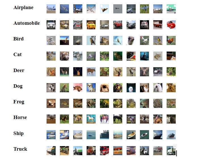
In one of our previous posts Data Loaders with PyTorch we already explained how we can work with the CIFAR10 dataset. Just to remind you, this dataset consists of 60,000 colored (RGB) images of dimensions \(32\times32 \) pixels divided into 10 classes (6,000 images per class). The dataset is divided into five training batches and one test batch, each with 10,000 images. In the following image, we can see 10 classes of the dataset, as well as 10 random images from each class.

Now, let’s start to load our dataset and explore the data.

2. Exploring CIFAR10 dataset images

First, we will import the necessary libraries with the following code.

import torch
import torch.nn as nn
import torch.nn.functional as F 

from torchvision import datasets, transforms
from torch.utils.data import DataLoader
from sklearn.metrics import confusion_matrix

import matplotlib.pyplot as plt
import numpy as npCode language: JavaScript (javascript)

Before we download the CIFAR10 dataset, we need to convert images from the dataset to PyTorch tensors. The way to do that is to create a variable transform and apply the function transforms.ToTensor().

transform = transforms.ToTensor()

To automatically download the CIFAR10 dataset we will create a variable and use a simple string (these two dots mean that we are going one level up from the current directory) to specify the path. Next, we create an object cifar10_train and from datasets, we call the function CIFAR10(). As arguments to this function, we will provide data_path, train which is set to True because this part of the data set will be used for training purposes. The third argument is a download which is also set to True. Then, with the same function, we will create an object cifar10_test where testing data will be stored. The only difference is that here, we will set the argument train to False. This means that this data set will not be used for training purposes, but for testing.

data_path = '../data_cifar/'
cifar10_train = datasets.CIFAR10(data_path, train=True, download=True, transform=transform)
cifar10_test = datasets.CIFAR10(data_path, train=False, download=True, transform=transform)Code language: PHP (php)

Now, if we check our training and testing data, we can see that variable cifar10_train consists of 50,000 images and variable cifar10_test consists of 10,000 images. We can check the type of the image with the function type() and we will see that it is a PIL image.

print("Training: ", len(cifar10_train))
print("Testing: ", len(cifar10_test))Code language: PHP (php)

Training: 50000

Testing: 10000

Now, let’s go ahead and examine our data in more detail.

If we check the type of our training data we can see that it is a very specific torchvision data type. Basically, this torchvision.datasets.cifar.CIFAR10 is a collection of tensors organized together.

type(cifar10_train)

torchvision.datasets.cifar.CIFAR10

type(cifar10_test)

torchvision.datasets.cifar.CIFAR10

By using indexing we can get back a tensor as an output. What is interesting here is that this is a tuple of two items. The first item is a \(32\times32 \) pixel image, and the second item is the label. Now we unpack this tuple and check the type and shape of one image.

type(cifar10_train[0])Code language: CSS (css)

tuple

image, label = cifar10_train[0]
type(image)

torch.Tensor

image.shapeCode language: CSS (css)

torch.Size([3, 32, 32])

We can see that image is a tensor of \(3\times32\times32 \) where number 3 represents three channels of red, green, and blue color and \(32\times32 \) pixels is the size of the image.

Also, if we print classes and the label. We can see that the value of the label is 6. If we take a look at the class names we will see that it is a frog.

classes = cifar10_train.classes
print (classes)
print(label)
print(classes[label])Code language: PHP (php)

Output:

('plane', 'car', 'bird', 'cat', 'deer', 'dog', 'frog', 'horse', 'ship', 'truck')
6
frogCode language: JavaScript (javascript)

Now, let’s visualize one image from our dataset. Note that order of the dimensions is \(3\times32\times32 \). However, to plot the image with Matplotlib the order should be \(32\times32\times3 \). So, to change the order of the dimensions we will use the function permute().

plt.imshow(image.permute(1, 2, 0))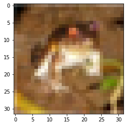Code language: CSS (css)

It is important to understand that to build the Neural Network we will work with a large number of parameters. For this reason, it makes sense to load training data in batches using the DataLoader class. What we are going to do is to grab a subset of 60,000 images using the following code.

torch.manual_seed(80)
train_loader = DataLoader(cifar10_train, batch_size=100, shuffle=True)
test_loader = DataLoader(cifar10_test, batch_size=500, shuffle=False)Code language: PHP (php)

Here, we are using the function manual_seed() which sets the seed for generating random numbers. Then we are going to create train_loader and test_loader objects using the function DataLoader().

For the train_loader object as parameters, we will pass our training data cifar10_train and batch_size that will automatically group images into batches. For this example, we will use a batch size of 100. The last parameter is shuffle which will shuffle our data after we pass the boolean value of True.

Then, we create a test_loader using the same code. The only difference is that we don’t really need to shuffle the data. That is why the shuffle parameter will be set to False. Also, a batch_size for a test_loader will be equal to 500.

Now, when we explored the data of the CIFAR10 dataset let’s move on to building our Neural Network.

3. Building the model

First, we will create the model class the MultilayerPerceptron() using nn.Module method. After that, we will set up the initialization method _init_. As parameters, we will pass self and input_size. Remember, we need to flatten out our images before feeding them into the Neural Network. The size of the images in the CIFAR10 dataset is \(3\times32\times32 \) pixels and that is equal to 3,072. This number will be the size of the initial inputs. We will also define the output size where we should have 10 neurons (each neuron will represent one class of the CIFAR10 dataset). Note that an Artificial neural network has only three layers of neurons. First, we have an input layer, one hidden layer, and the output layer that generates predictions.

Finally, we will define the size of the three layers. The size of the input layer will be equal to the size of the initial inputs which is 3,072 neurons. Then, we will set the size of two hidden layers of size 120, and 84 neurons, and the size of the output layer will be 10 neurons. It is important to note that in this case, the number of layers represents the number of weight matrices \(W \). So, this will be a three-layer Artificial Neural Network.

class MultilayerPerceptron(nn.Module):

    def __init__(self, input_size=32*32*3, output_size=10):
        super().__init__()
        self.fc1 = nn.Linear(input_size, 120)
        self.fc2 = nn.Linear(120, 84)
        self.fc3 = nn.Linear(84, output_size)
        #self.dropout = nn.Dropout(p=0.5)

    def forward(self, X):
        X = F.relu(self.fc1(X))
        X = F.relu(self.fc2(X))
        X = self.fc3(X)

        return F.log_softmax(X, dim=1)

Next, we can start to specify the size of connected linear layers. Once we do that we will define a forward method. It is important to note that here we need to choose the activation function which will be used in the hidden layers as well as at the output unit of the Neural Network. As an activation function, we will choose Rectified Linear Units (ReLU for short). So, once again, we will take our data and pass it to the first fully connected layer. Then, we will apply the activation ReLu function, take that result and pass it to the second layer. We will repeat the same process once again. Finally, we will take that result and pass it through the logarithmic softmax activation function log_softmax(). As parameters to this function, we will pass x and we will specify the dimension along which log_softmax() will be calculated. In this case, this dimension should be equal to 1.

Now, let’s move ahead and set seed once again. Then, we will create a variable model which will be used for calling our MultilayerPerceptron class.

torch.manual_seed(80)
model = MultilayerPerceptron()
model

Output:

MultilayerPerceptron(
  (fc1): Linear(in_features=3072, out_features=120, bias=True)
  (fc2): Linear(in_features=120, out_features=84, bias=True)
  (fc3): Linear(in_features=84, out_features=10, bias=True)
)Code language: PHP (php)

Here we can see our MultilayerPerceptron model. Now, it is important to point out here that in some of the future posts we are going to tackle the same problem, but using a Convolution Neural Network. One of the main motivations to use a CNN is the number of parameters that an artificial Neural Network has compared to a CNN. The CNN architecture is going to be more efficient and it will have significantly fewer parameters.

So, let’s create the for loop and check the total number of parameters in the model.parameters() We can extract the number of elements using the function param.numel().

for param in model.parameters():
  print(param.numel())Code language: CSS (css)

Output:

And here you can see, we get a huge number of parameters. First, we have 368,640 connections from 3,072 to 120. Then, we have the 120 biases. Next, we have all connections into that next layer, and so on. If we were to sum these parameters up, we will see that we actually end up with 379,774 total parameters. In some of the future posts, we are going to see that we’re gonna have much fewer parameters if we use a more efficient CNN. So, this could be a motivation for moving to CNN, especially when dealing with image data.

Now, let’s complete our network by defining a loss function and an optimizer. First, we will create a criterion and calculate the loss by using the function nn.CrossEntropyLoss() We will apply this particular function because this is a multi-class classification problem.

Then, we will create a variable optimizer, and call the function torch.optim.SGD() which will calculate the gradients. (SGD stands for Stochastic Gradient Descent). Then, we will pass model.parameters() that we want to update. Also, we will set the learning rate to be equal to 0.01.

criterion = nn.CrossEntropyLoss()
optimizer = torch.optim.SGD(model.parameters(), lr=0.01)

The last thing that we are going to do before moving on to the training part is to transform the entire dataset with a command view(). This function keeps three channels and merges all the remaining dimensions into one dimension with the appropriate size. Here, images of dimensions \(64\times3\times32\times32 \) (64 is the batch size, 3 is the number of channels, and \(32\times32 \) is the size of an image) are transformed into dimensions of \(64\times 3072 \).

for images, labels in train_loader:
  breakCode language: JavaScript (javascript)

images.shapeCode language: CSS (css)

torch.Size ([64, 3, 32, 32])

images.view(-1, 3072).shapeCode language: CSS (css)

torch.Size ([64, 3072])

Once we have built our Neural Network the next step is to train the model. Let’s see how we can do that.

4. Training the model

The first thing that we want to do is to import time. In that way, we can set up a start_time, and then at the end, once training is finished we will calculate and print the time that has elapsed.

import time
start_time = time.time()Code language: JavaScript (javascript)

Now, let’s set up our training. First, we will set the number of epochs to 10. For this dataset, this is the optimal amount of training.

epochs = 10

train_losses = []
test_losses = []
train_correct = []
test_correct  = []

Next, we will create an empty list train_losses so that we can keep track of the loss during training. Also, we will create another empty list test_losses so that we can evaluate the train and test loss as we train for more and more epochs. Furthermore, we also need to keep track of what we got correct. For this, we’ll create empty lists train_correct and test_correct.

Now it’s time for the actual training. We will create a for loop that will iterate in the range of epochs. Then, we’ll set trn_corr and tst_corr to start off from zero.

for i in range(epochs):
   
    trn_corr = 0
    tst_corr = 0

Then, we’ll run the training batches. We’ll create a for loop and use the enumerate() method to iterate over X_train and y_train. As an argument to the enumerate() function, we will pass train_loader. Remember that the train_loader returns back the image and its label. Therefore, with the enumerate() function we are going to keep track of batch numbers.

for b_iter, (X_train, y_train) in enumerate(train_loader):
      b_iter +=1

      y_pred = model(X_train.view(100, -1))
      loss = criterion(y_pred, y_train)
      
      predicted = torch.max(y_pred.data, 1)[1]
      batch_corr = (predicted == y_train).sum()
      trn_corr += batch_corr
      
      
      optimizer.zero_grad()
      loss.backward()
      optimizer.step()

Next, we will say that b_iter is equal to += 1. The reason for that is that batch number starts at zero and that doesn’t really make sense. So, we are doing this in order to set the batch number to start at one.

Then, we are going to set the prediction of the model. We will pass X_train and with command .view() we will flatten out the images. We also need to calculate the loss which is equal to the criterion of predicted values and original values.

The next step is to extract maximal predicted values. The idea behind that is pretty simple. Recall that in the last layer, we have 10 neurons. These neurons are essentially going to output probabilities per class. Eventually, one of these neurons is going to have the maximal value. So, we want to grab that maximal value along the correct axes. This is essentially the transformation of these probabilities into the labels.

Then, we can say that batch_corr is equal to a variable predicted that is equal to y_data and we can take the sum of this.

The next step is to apply backpropagation and optimize our parameters. To calculate the gradients we will use the optimizer.step() function . Remember that we need to make sure that calculated gradients are equal to 0 after each epoch. To do that, we’ll just call optimizer.zero_grad() function.

The next thing that we want to do is to print some results during the training. So we’ll go ahead and say if the batch numbers divided by 100, are equal to zero, we’ll go ahead and print the epoch, bach, loss, and accuracy. We are going to calculate accuracy separately. So we can say accuracy is equal to the total_train_loss multiplied with 100 and divided by total_trained.

if b_iter % 100 == 0:
        
        accuracy = trn_corr.item()*100 / (100*b_iter)
        print( f'epoch: {i} batch {b_iter} loss:{loss.item()} accuracy:{accuracy} ')Code language: PHP (php)

Next, what we want to do is update the training, loss, and accuracy for each epoch. For that, we will append loss and trn_corr to the lists that we created outside of the for loop.

train_losses.append(loss)
train_correct.append(trn_corr)Code language: CSS (css)

So, that is the code that takes care of the training data. Now, we need to run our test data during the training. This will allow us to understand how our test validation is going down. Eventually, after a certain number of epochs, we should see less return on the test data results versus the training results. The rest of the code will be exactly the same as for training only now we are going to use X_test and y_test.

with torch.no_grad():
      
      for b_iter, (X_test, y_test) in enumerate(test_loader):
        
        y_val = model(X_test.view(500, -1))
        
        predicted = torch.max(y_val.data, 1)[1]
        tst_corr += (predicted == y_test).sum()
     
    loss = criterion(y_val,y_test)
    test_losses.append(loss)
    test_correct.append(tst_corr)Code language: JavaScript (javascript)

Finally, we are going to print the time that we defined at the beginning of the training code.

    total_time = time.time() - start_time
    print( f' Duration: {total_time/60} mins')Code language: PHP (php)

For complete understanding, we will show the overall training code.

import time
start_time = time.time()

epochs = 10

train_losses = []
test_losses = []
train_correct = []
test_correct  = []

for i in range(epochs):
   
    trn_corr = 0
    tst_corr = 0
    batch_corr = 0
    

    for b_iter, (X_train, y_train) in enumerate(train_loader):
      b_iter +=1

      y_pred = model(X_train.view(100, -1))
      loss = criterion(y_pred, y_train)
      
      predicted = torch.max(y_pred.data, 1)[1]
      batch_corr = (predicted == y_train).sum()
      trn_corr += batch_corr
      
      
      optimizer.zero_grad()
      loss.backward()
      optimizer.step()

      if b_iter % 100 == 0:
        
        accuracy = trn_corr.item()*100 / (100*b_iter)
        print( f'epoch: {i} batch {b_iter} loss:{loss.item()} accuracy:{accuracy} ')
    
    train_losses.append(loss)
    train_correct.append(trn_corr)

    with torch.no_grad():
      
      for b_iter, (X_test, y_test) in enumerate(test_loader):
        
        y_val = model(X_test.view(500, -1))
        
        predicted = torch.max(y_val.data, 1)[1]
        tst_corr += (predicted == y_test).sum()
     
    loss = criterion(y_val,y_test)
    test_losses.append(loss)
    test_correct.append(tst_corr)

total_time = time.time() - start_time
print( f' Duration: {total_time/60} mins')Code language: JavaScript (javascript)

So, lets train our model and check the results.

5. Evaluating the results

Now that our model is trained, let’s take a look at the overall evaluation and performance of both the training set and the test set.

So, let’s plot the loss and accuracy comparisons of the training and validation data. First, we will plot the train_losses and the thest_losses.

plt.plot(train_losses, label= "Training loss")
plt.plot(test_losses, label= "Test loss")
plt.legend()Code language: JavaScript (javascript)

Output:

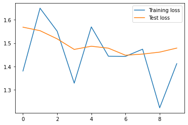
As you can see, as we train for more epochs the train_losses tends to decrease. On the other hand, we are not performing as well on the test_losses. However, this makes perfect sense because it is the data that Neural Network has never seen before. That is why we can’t expect to perform as well as it did on the training set.

Now, let’s plot accuracy comparisons of the training and validation data. First, we will take a look at the train_accuracy. Note that if we just print this variable we will get the number of correctly predicted data in each epoch. Now, we can divide all data in the training set (50,000 images) by 500 which will give us the percentage of correctly predicted data. We will do the same thing for the training and testing data.

train_accuracy =[t/500 for t in train_correct ] 
train_accuracy

Output:

[tensor(43.2300),
 tensor(45.1480),
 tensor(46.3600),
 tensor(47.5360),
 tensor(48.2500),
 tensor(48.7520),
 tensor(49.4980),
 tensor(50.1300),
 tensor(50.6140),
 tensor(51.2020)]Code language: JSON / JSON with Comments (json)

test_accuracy =[t/100 for t in test_correct ] 
test_accuracy

Output:

[tensor(44.0700),
 tensor(44.8600),
 tensor(46.2700),
 tensor(47.3400),
 tensor(46.9200),
 tensor(47.3800),
 tensor(48.2700),
 tensor(48.6900),
 tensor(47.5000),
 tensor(48.3300)]Code language: JSON / JSON with Comments (json)

As you can see, the percentage of correctly predicted data is getting larger after each epoch. However, the accuracy is just 48%. So, we can conclude that our Fully Connected model does not perform so well on the CIFAR10 dataset. For better results, we need to use Convolutional Neural Network.

Now, lets plot the train_accuracy and test_accuracy.

plt.plot(train_accuracy, label= "Training accuracy")
plt.plot(test_accuracy, label= "Test accuracy")
plt.legend()Code language: JavaScript (javascript)

Output:

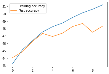
As you can see the train_accuracy is going to increase as we train for more epochs. On the other hand, the test_accuracy is going to level up at some point. This could be a good indication of how many epochs we should use for training this dataset. Because once we reach the point where test_accuracy is going to level up there is no point to train for more epochs.

One interesting question is how we can run new image data through our trained model? To do that, we first need to evaluate the test data separately by extracting all test data at once. We will use the same code as before only now we will set the batch_size the parameter to 10.000 which is the number of test images in the CIFAR10 dataset.

test_load_all = DataLoader(cifar10_test, batch_size=10000, shuffle=False)Code language: PHP (php)

Now, let’s evaluate new unseen images. For that, we will create a similar for loop as we did in the training process. However, this time we will load all 10.000 images from the CIFAR10 dataset.

with torch.no_grad():
  correct = 0
  for X_test, y_test in test_load_all: 
    y_val = model(X_test.view(len(X_test),-1))
    predicted = torch.max(y_val,1)[1]
    correct += (predicted == y_test).sum()Code language: JavaScript (javascript)

We can print the percentage of correctly predicted data with the following code.

100*correct.item()/len(cifar10_test)

48.3

Again, you can see that the accuracy is the same.

One additional thing that we can do is to display a confusion matrix. A confusion matrix, also known as an error matrix, is a specific table layout that allows visualization of the performance of an algorithm.

confusion_matrix(predicted.view(-1),y_test.view(-1))Code language: CSS (css)

Output:

array([[581,  84,  75,  50,  65,  44,  13,  58, 125,  74],
       [ 12, 417,  13,   6,   4,   4,   3,   3,  31,  92],
       [ 80,  13, 356,  90, 125, 102,  47,  87,  28,  22],
       [ 46,  47, 118, 399,  80, 267, 102,  95,  43,  64],
       [ 50,  28, 181,  65, 448,  74, 114, 116,  31,  21],
       [ 10,  17,  47, 114,  22, 306,  25,  53,  14,  15],
       [ 25,  29, 128, 175, 165, 122, 659,  49,   9,  44],
       [ 26,  34,  46,  39,  59,  48,  16, 489,  15,  38],
       [139, 126,  21,  24,  22,  18,  10,  17, 657, 109],
       [ 31, 205,  15,  38,  10,  15,  11,  33,  47, 521]])Code language: CSS (css)

Here, each column represents a class of a dataset and on diagonals, we can see how much data is pres class is predicted correctly.

Now, we will check the prediction for one image from the dataset. We will create a variable model_prediction and apply the function model_forward() on the image. In that way, we will extract a raw prediction of how much our Neural Network thinks that an image corresponds to a certain class. These predictions will be used as an input for the softmax() function.

img = images[0].view(1, 3072)

# we are turning off the gradients
with torch.no_grad():
    model_prediction = model.forward(img)Code language: PHP (php)

probabilities = F.softmax(model_prediction, dim=1).detach().cpu().numpy().squeeze()

print(probabilities)

fig, (ax1, ax2) = plt.subplots(figsize=(6,8), ncols=2)
img = img.view(3, 32, 32)
ax1.imshow(img.permute(1, 2, 0).detach().cpu().numpy().squeeze(), cmap='inferno')
ax1.axis('off')
ax2.barh(np.arange(10), probabilities, color='r' )
ax2.set_aspect(0.1)
ax2.set_yticks(np.arange(10))
ax2.set_yticklabels(np.arange(10))
ax2.set_title('Class Probability')
ax2.set_xlim(0, 1.1)

plt.tight_layout()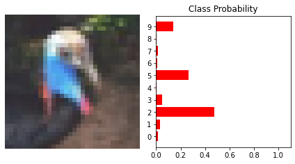Code language: PHP (php)

As you can see, our model classifies the bird as a class 2 which is correct. However, the probability is just 50%. It also classifies this image as a class 5 (deer) with a probability of 30% and class 9 (truck) with a probability of 20%,

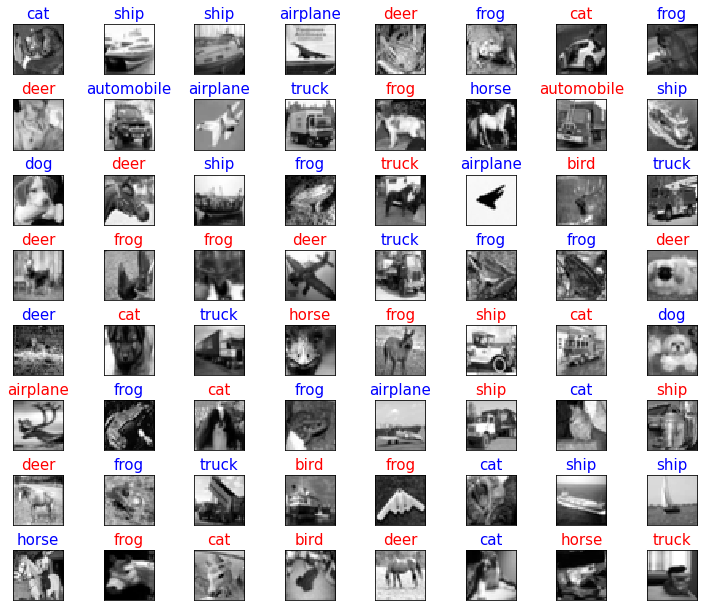
Finally, let’s plot our images and the predictions. If the prediction is correct the label above the image will be colored in blue, and if the prediction is incorrect the label will be colored in red.

test_load_all = DataLoader(cifar10_test, batch_size=64, shuffle=False)Code language: PHP (php)

images, labels = next(iter(test_load_all))

with torch.no_grad():
  images, labels = images, labels
  preds = model(X_test.view(len(X_test),-1))

images_np = [i.mean(dim=0).cpu().numpy() for i in images]
class_names = cifar10_test.classesCode language: JavaScript (javascript)

fig = plt.figure(figsize=(10, 8))
fig.subplots_adjust(left=0, right=1, bottom=0, top=1, hspace=0.5, wspace=0.05)

for i in range(64):
    ax = fig.add_subplot(8, 8, i + 1, xticks=[], yticks=[])
    ax.imshow(images_np[i], cmap='gray', interpolation='nearest')
    color = "blue" if labels[i] == torch.max(preds[i], 0)[1] else "red"
    plt.title(class_names[torch.max(preds[i], 0)[1]], color=color, fontsize=15)Code language: JavaScript (javascript)

So, we can see that our model predicted just 50% of the data correctly.

Click here to get PyTorch code !

Summary

In this post, we have learned how to train our model and make accurate predictions for the CIFAR10 dataset. We showed you how to build a Neural Network that can correctly predict the data with an accuracy of over 90%. In the next post, we are going to talk about data normalization.

#010 PyTorch – Artificial Neural Network with Perceptron on CIFAR10 using PyTorch