#011 Pytorch – RNN with PyTorch

Highlights: In this post, we will give a brief overview of Recurrent Neural Networks. Along with the basic understanding of the RNN model, we will also demonstrate how it can be implemented in PyTorch. We will use a sine wave, as a toy example signal, so it will be very easy to follow if you are encountering RNNs for the first time. Let’s start with our post!
Tutorial Overview:
- Introduction to Recurrent Neural Networks
- Introduction to Long Short Term Memory-LSTM
- RNN/LSTM model implemented with PyTorch
1. Introduction to Recurrent Neural Networks
Fully Connected Neural Networks or Convolutional Neural Networks mainly work with vector data types and images. However, not all data can be effectively presented in this way. For instance, text or time series are better modeled as time sequences. So, in this post, we will see how time series can be modeled and forecasted using Recurrent Neural Networks.
One example of sequence signals are physiological signals such as heart rate or pulse. These signals can be used for classification or prediction. For instance, you can have a signal with certain patterns in healthy patients. And then, you will have a similar recording of an unhealthy subject. Then, you can train your model to determine whether the person is sick or healthy. For example, we can determine whether a person has an arrhythmia or not. The recordings may last for 24 hours, so it is impractical for a human observer / medical doctor to examine all this data, and therefore, a computer-assisted solution in terms of Recurrent Neural Networks can be a way to predict this.
On the other hand, you can maybe have an outbreak of COVID-19 cases and you want to predict the trend of growth or decline of the new patients or a death rate. Another example can be travelers who are going to visit a certain country during summertime. In that case, you would like to have data from the previous five years during summertime and also the situation prior to summer in order to track the trend of that current year. In case that the external factors are not changing a lot, your model can make meaningful predictions.
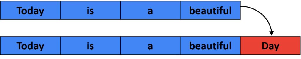
Last but not least, you can model text as a sequence. Have a look at the example below, where you are trying to predict the next word for a given sequence.
So, in this post, we will start with a very brief RNN theory that we also covered in a series of posts [1, 2, 3, 4, 5] together with the LSTMs and Gated Recurrent Units (GRU). Then, we will see how we can perform some simple implementation of a Time series prediction using RNN.
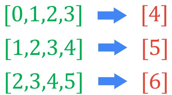
The main idea of predicting a sequence is that you will have several sequence elements as input. For instance, you can have a sequence \([1, 2, 3, 4] \), then, one step into the future you would like to predict the unknown value.
So, you can use Bitcoin’s price from the last 4 days, and then, you want to predict tomorrow’s price. One example of a time series is the following graph for the Bitcoin price change from June 2018.

So, the main idea of models is that within Recurrent Neural Networks, we will have a neuron that should know about its previous outputs. A simple way to do this is just to feed its output back to itself. In the following image, we can see an example of one simple neuron in Feed-Forward Networks where we had the aggregation of input and output from the previous time step.
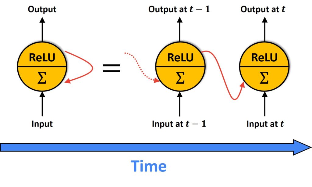
Therefore, in the recurrent neuron, we send the output back to itself. So, here, we can have a situation where we have input at the time instance \(t-1 \) which will give us an output at \(t-1 \). Then, at the next time instance, we will have an input at time \(t \), plus the outputs from the previous time instance. That output is \(t-1 \), and then it will give us an output at \(t \). So, we can treat this as a simple Feed-Forward Network, but keep in mind that the input will have an output from the previous sequence. Here, the cells that are a function of inputs from the previous time steps are also known as the memory cells.
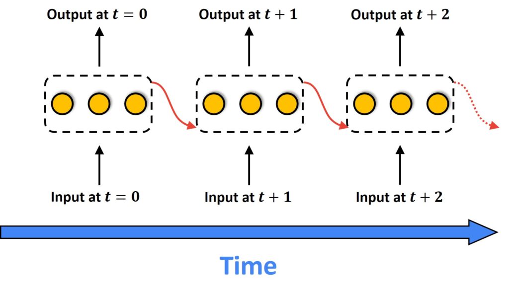
Next, we have an example of an RNN layer with three neurons. The output here is going back as an input to all three hidden neurons. One common procedure that we do is to unroll an RNN in time. Observe in the image below how this network structure now looks like.
There are several different types of Recurrent Neural Networks. We can categorize RNN architectures into the following four types:
- Many-to-many
- Many-to-one
- One-to-one
- One-to-many
For example, we can have a sequence to sequence type – many-to-many.
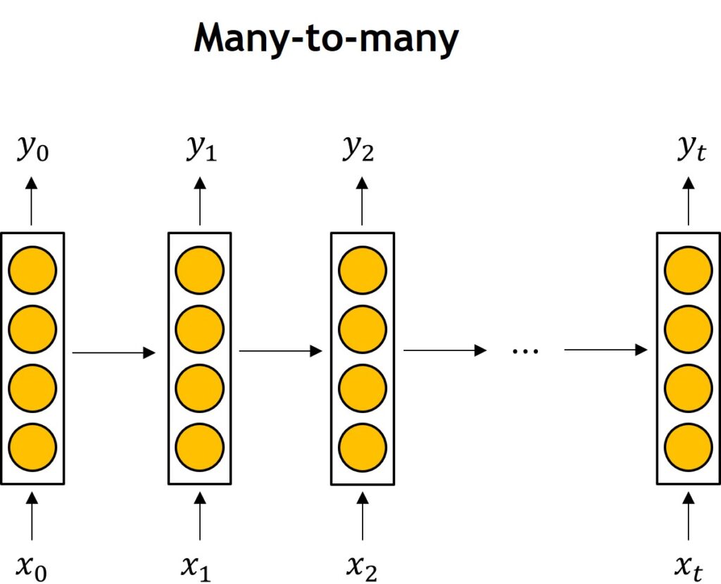
In this case, you will have five words and you have to predict the next five words.
Another common type of RNNs is many-to-one where we start with a sentence of five words we will end up with the one output.
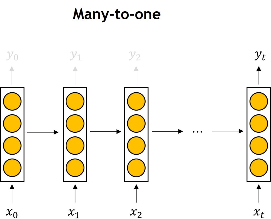
This type of RNN can be used when we have five words in a sentence and we want to predict the word that most likely follows these five words. An example can be a model that has to learn and to provide the following word as the output while you type on your smartphone.
One shortcoming of the RNN models is that we don’t want to have only short-term memory. We would like to have models that would work much better if we are able to track a longer history in time. Also, there is one problem with the training which is known as “vanishing gradient”. Further in the post, we will see how they can be improved in models known as LSTM (Long Short Term Memory) Units.
To better understand the vanishing gradients let’s take a look at the following image.
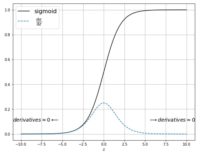
Here, we can see the sigmoid function in black, and the sigmoid derivative in blue. We can see that values lower than -5 and higher than +5 are practically already zero. In such a case the gradients cannot propagate well due to small values. That is the reason why we call them a vanishing gradient. Therefore, training of the time-related sequences can be a problem.
2. Introduction to Long Short Term Memory – LSTM
Now, let’s have a look into LSTMs and GRU (Gated Recurrent Units). So, this was the main bottleneck of RNNs because it tends to forget very quickly. The information is lost when we go through the RNN, and therefore, we need to have a mechanism to provide a long-term memory for our models. The cell, known as Long-Short-Term Memory, can assist us to overcome the disadvantages of an RNN. In the following image, we can see a typical unrolled RNN.
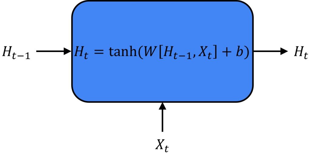
Usually this output \(t-1 \) is called hidden state- \(H_{t-1} \). Also, it gives the output as a hidden state \(H_{t}\). We can treat this as a simple neuron that we’ve seen in fully connected neural networks. However, here, this \(H_{t} \) is calculated using a hyperbolic tangent. Basically, here we have a matrix of coefficients or weight matrix \(W \) that multiplies \(H_{t-1} \) and the input vector \(X_{t} \). Also, we have a bias term \(b \). So, that’s how we obtain the output \(H_{t} \).
On the other hand, with LSTMs we will have something different. Here, we can see two signals called Short Term Memory and Long Term Memory.
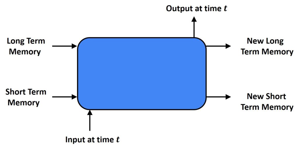
Here, the input at time \(t \) will provide the output at time \(t \), but it will also keep track of current and updated Short Term Memory as well as the current and an updated New Long Term Memory. Furthermore, there are four gates here: Forget gate, Input gate, Update gate, and Output gate.
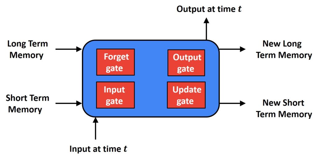
All these four gates are very important. They pass information if the signal value is close to one, and they will not pass forward the information if it is close to zero.

Here, \(\sigma \) stands for sigmoid and \(tanh \) is hyperbolic tangent. Also, we create \(f_{t} \) which is a sigmoid of the following multiplication plus \(b_{f} \).
$$ f_{t}=\sigma\left(W_{f} \cdot\left[h_{t-1}, x_{t}\right]+b_{f}\right) $$
Then, we have a signal \(i_{t} \) which is a sigmoid of the following multiplication:
$$ i_{t}=\sigma\left(W_{i} \cdot\left[h_{t-1}, x_{t}\right]+b_{i}\right) $$
Then of course, we have a signal \(\tilde{C}_{t} \) which can be calculated in the following way:
$$ \tilde{C}_{t}=\tanh \left(W_{C} \cdot\left[h_{t-1}, x_{t}\right]+b_{C}\right) $$
Next, we obtain a signal \(C_{t} \):
$$ C_{t}=f_{t} * C_{t-1}+i_{t} * \tilde{C}_{t} $$
The first part of an equation is element wise multiplication, and then, we add signal \(i_{t} \) multiplied with \(\tilde{C}_{t}\).
Finally, we will obtain \(o_{t}\) and \(h_{t} \) as follows:
$$ o_{t}=\sigma\left(W_{o}\left[h_{t-1}, x_{t}\right]+b_{o}\right) $$
$$ h_{t}=o_{t} * \tanh \left(C_{t}\right) $$
Now, let’s explain this in more detail. In the image above we can see that the \(C_{t} \) signal goes down and passes through \(tanh \). Then, we have the output at the time \(t \), \(o_{t} \). These two signals are multiplied, using the so-called, element-wise multiplication, and we finally obtain the signal \(h_{t} \).
Fortunately, we have Deep Learning libraries like PyTorch or TensorFlow, so we don’t have to code all these equations on our own. We can just use them and apply them for our purposes. Before we proceed, let’s discuss how the data should look like for this model. A time-series usually looks like this: we have a sequence that is separated into two parts. We have a training sequence and the sequence value that should be predicted/forecasted.
For instance, we can have a set of numbers \([1,2,3,4,5] \). Then, for the training batch, we will use \([1,2,3,4] \) and for the desired output we will have \([5] \).
Therefore, we usually train sequences using batches. We can edit the size of the training data point, as well as how many sequences we want to feed per batch.
One interesting thing is that when we work with predictions a common way to estimate our error would be Root Mean Square Error ( RMSE ). Using this approach we can measure how good our prediction is.
Usually, once we have our data, we save the last 10% or 20% of our time series for the test. Next, we use the previous part for training and to run predictions. Then, the last part we use for the test to see how well we are performing.
An interesting event occurs when we select the last part of the sequence – the last remaining batch.
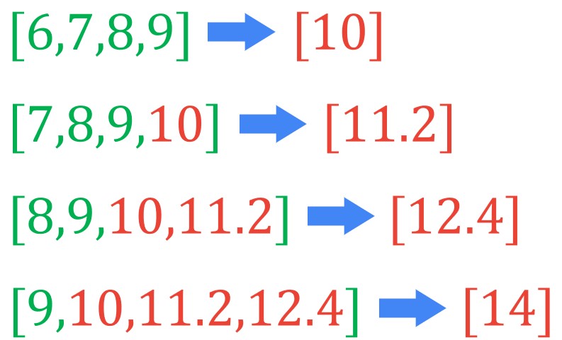
Then, we can use this predicted number 10. We can say that this will be a value of Bitcoin for tomorrow, and then we will predict the value of two days after today. After that, we can use that value and place it in the third sequence and once again calculate the output of the prediction. Finally, we will move our sliding window and we will have three numbers that we’ve already predicted. We will use this whole sequence to predict the final output. Of course, since all of these numbers are predictions they will have an error and that error will propagate through this more and more. Eventually, the longer we do these predictions without recording data, we will have more inaccurate predictions. That means that if we want to predict bitcoin price for five days, we can be reasonably successful. However, if we want to predict it for one year, our predictions will probably not be valid at all.
Now, let’s apply this knowledge in Python.
3. RNN/LSTM model implemented with PyTorch
First, let’s import necessary libraries.
import torch
import torch.nn as nn
import numpy as np
import pandas as pd
import matplotlib.pyplot as plt
Next, will define x as an array of numbers from 0 to 799. Then we define a simple sin using the command torch.sin(). We will take \(x\cdot 2\pi \) and we will divide this with 40 in order to achieve higher frequency.
Creating a dataset
x = torch.linspace(0,799, 800)
y = torch.sin(x * 2 * np.pi / 40)
With the following code, we can plot these values.
plt.figure(figsize = (12,4))
plt.xlim(-10, 801)
plt.grid(True)
plt.plot(y.numpy() )
Then, we will use a size of 40 which means that our test will consist only of 40 elements. Also, we will split our data into train_set and test_set, so that train_set will go from 0 to 759, and test_set will have the last 40 elements.
test_size = 40
train_set = y[:-test_size]
test_set = y[-test_size:]
We can plot these values and this is how they look.
plt.figure(figsize = (12,4))
plt.xlim(-10, 801)
plt.grid(True)
plt.plot(train_set.numpy())
So, this is the train_set consisting of all the elements without the last 40 elements.
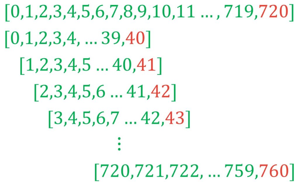
Now, this function is doing something interesting. As parameters, we will pass here an input sequence and window size. In our case, the window size will be 40. This function takes the length of a sequence minus window size. For example, if the window size is 40 our input training set will be 760 elements. So, this loop will go from 0 to 719. So, we can print this just to be sure.
def input_data(seq, ws):
  output = []
  L = len(seq)
  for i in range((L) - ws):
    window = seq[i:i+ws]
    label = seq[i+ws:i+ws+1]
    print(i)
    output.append((window, label))

  return output
The idea here is that we will loop over these elements and basically, we will start from zero and then go up to forty elements. So, this will be located in zero variable. Then we will have a label that will be exactly the element after the windows sequence. So, if we have 40 here this will be the 41st element. Then we will append only the window and this label in a tuple. So this will be a list consisting of tuples.
Next, we define window_size to 40, and call this input_data with train_set and window_size. We will obtain train_data like a batch.
window_size = 40
train_data = input_data(train_set, window_size)
Output:
0,1,2,3,...719As you can see the loop will go up to 719. So basically train_data will be equal to 720 sequences, where each of them consists of 40 elements and the next value that needs to be predicted.
The first element from train_data will have the first 40 elements of our sin signal. Then the 41st element will be the value that we want to predict. We can visualize one sequence using the function plt.stem().
plt.stem(train_data[0][0])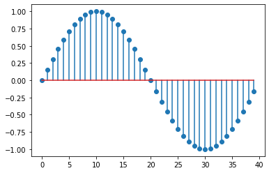
Defining the LSTM model using PyTorch
Now, we will continue with our code by looking at the class torch.nn.LSTMCell. Here we can see what this function is calculating for us:
$$ i=\sigma\left(W_{i i} x+b_{i i}+W_{h i} h+b_{h i}\right) $$
$$ f=\sigma\left(W_{i f} x+b_{i f}+W_{h f} h+b_{h f}\right) $$
$$ g=\tanh \left(W_{i g} x+b_{i g}+W_{h g} h+b_{h g}\right) $$
$$ o=\sigma\left(W_{i o} x+b_{i o}+W_{h o} h+b_{h o}\right) $$
$$ c^{\prime}=f * c+i * g $$
$$ h^{\prime}=o * \tanh \left(c^{\prime}\right) $$
Here \(\sigma \) is the sigmoid function and the asterisk sign is the Hadamard product also known as an element-wise multiplication.
So, these are the equations that we had for torch.nn.LSTMCell. Note here that bias can be set to True or False and the default value is True. So, we will leave it as such. The input consists of three terms. We have a common input, and then we have two more inputs, which are passed as a tuple: hidden state h_0, and cell state h_c. In this case, h_0, and h_c are initial states for each element in the batch.
For the output, we have something similar. We will have a tuple of a New long-term memory and a New short-term memory, and also we will have an output vector as well.
torch.nn.LSTM(input_size, hidden_size)Now, we will create an LSTM model by creating our class. We will call it myLSTM and we will derive all the members from the nn.module. So, we will have an init function with the following parameters: self, input_size which will be equal to 1, hidden_size which will be equal to 50, and out_size which we will set to 1. So, you can think of a hidden_size as the number of neurons in a hidden LSTM layer.
Next, we will call super() and we will instantiate from the class that we are calling on. This means that in nn.module we will have available all functions, parameters, and methods developed in the initial part.
We will start by defining the hidden_size. In this case, we will also go from hidden_size to the output_size. Here we select that hidden_size is equal to 50. Then, we will go from the LSTM layer to the output layer using a well-known, fully connected layer.
class myLSTM(nn.Module):
  def __init__(self, input_size=1, hidden_size=50, out_size=1):
    super().__init__()
    self.hidden_size = hidden_size
    self.lstm = nn.LSTM(input_size, hidden_size )
    self.linear = nn.Linear(hidden_size, out_size)
    self.hidden = (torch.zeros(1,1,hidden_size ) , torch.zeros(1,1,hidden_size)  )

  def forward(self, seq):
    lstm_out, self.hidden = self.lstm(seq.view( len(seq),1,-1 ), self.hidden )
    pred = self.linear(lstm_out.view(  len(seq) ,-1 ))
    return pred[-1]
Now, with the parameter self.hidden, we will initialize this hidden layer. Those are values h_t and c_t in mathematical formulas. Note that now we initialize h_t and c_t as zeros. So, we will start the initial state of our LSTM, with zero values.
Next, we will define the forward method with self and seq as parameters. So, the seq variable will be the sequence that we work with within this class.
So, our first call will be self.lstm() layer and as the output, we will provide two parameters. The first parameter will be lstm_out which is an output of the LSTM. Then, we have self.hidden parameters which will also be updated as a tuple. Next, we also have h_t and c_t variables that we use in this function. We can also see that this function has to provide the input to the LSTM layer that now will be h_0 and c_0.
So, an input will be a sequence. We need to make sure that the sequence is of adequate shape. So, as parameters, we will have len(seq) and then we will have 1 and -1. The parameter self.hidden is just passed as self.hidden, where we have two values, h_t, and c_t.
Once we call the function lstm(), we will proceed by calculating a prediction. For that, we will use our linear layer. The input to this linear layer will be the output of the LSTM layer. Again, we need to make sure that it is of the correct shape. So, it will have the parameter len(seq) and we will include here -1 in case that we use batches. This -1 here stands that if we have an input system of, for instance, 32 batches, then instead of this -1, we will have a number 32.
Finally, we will return the prediction that is the last element of this sequence. For example, this prediction can be 1, 2, 3, 4. What we actually care about is the last element, pred[-1], that we are predicting. In this example, this is the number 4.
Next, let’s instantiate the model with myLSTM(). As we already said in the beginning, for the criterion we will use nn.MSELoss(). Next, for the optimizer, we will use the Stochastic Gradient Descent model by calling torch.optimSGD(). For this model, we will have an argument model.parameters(), and we will set the learning rate to 0.01.
model = myLSTM()
criterion = nn.MSELoss()
optimizer = torch.optim.SGD(model.parameters(), lr = 0.01)
print(model)
Output:
myLSTM(
  (lstm): LSTM(1, 50)
  (linear): Linear(in_features=50, out_features=1, bias=True)
)
This is how our model looks. We can see that first, we have an LSTM layer with 1 input and 50 hidden neurons. Then, it is followed by a linear layer and output features.
Next, what we can do is to go through all the model parameters and we can print the number of elements using the function p.numel().
for p in model.parameters():
  print(p.numel())
Output:
200
10000
200
200
50
1
Training the LSTM model in PyTorch
We have defined our model and now we need to train it. First, we will define the number of epochs and set it to 10. Then, we can use the parameter future and set it to 40. This parameter determines how many points we want to predict. This means that if we are dealing with the Bitcoin prices from today, we want to predict in the following consecutive 40 days what the daily price of bitcoin will be.
Then, for the number of epochs, we will create a for loop. The next step is to iterate over the train_data. What’s important here is that train_data will be a tuple of 40 numbers along with one output. That means that for the values of Bitcoin daily prices, we want to predict tomorrow’s price. We will set gradients to zero in our optimizer. Then we will set the model.hidden variable values to zeros. Note that there are two hidden vectors C_t and H_t. Finally, we will calculate y_pred, and we will define our loss. Here, the criterion is a root mean square error between the predicted value and train value that we have at the moment. The next step is to apply backpropagation through our network. Finally, we will call optimizer.step() in order to update our parameters.
epochs = 10
future = 40
for i in range(epochs):
  for seq, y_train in train_data:
    optimizer.zero_grad()
    model.hidden = (torch.zeros(1,1,model.hidden_size) ,
                    torch.zeros(1,1,model.hidden_size))

    y_pred = model(seq)
    loss = criterion(y_pred, y_train)
    loss.backward()
    optimizer.step()

  print(f"Epoch {i} Loss {loss.item()} ")
  preds = train_set[-window_size:].tolist()

  for f in range(future):
    seq = torch.FloatTensor(preds[-window_size:])
    with torch.no_grad():
      model.hidden = (torch.zeros(1,1,model.hidden_size) ,
                      torch.zeros(1,1,model.hidden_size))
      preds.append(model(seq).item())

  loss = criterion(torch.tensor(preds[-window_size :]), y[760:] )
  print(f'Performance on test range: {loss}')
Now, we will print our loss, and also we will obtain prediction values in a variable preds. We will do that in such a way that we will take the last window size elements. So, we will take the last 40 numbers using preds[-window_size :]
The next step is to create another for loop to iterate over the future parameter. Note here that we are taking the last 40 elements from the training set with window size. So, that’s defined with predictions train_set. That means that from these 40 elements, we are predicting tomorrow’s value. Then we will use this predicted value, we will append it, and then based on 39 values plus tomorrow’s predicted value we will predict the value in two days from today.
Next, we are defining a sequence. So, we will convert predictions into a torch. FloatTensor by taking the last window size elements. Then, we will exclude gradients to perform calculations. We will set model.hidden layers to zeros, and then we will calculate the predictions – preds. That is, to the predictions, we will append the values that we obtained from our model when our input is the seq array. Then, with the function .item() we will actually take these elements that will be appended into the prediction. So, because the output of the myLSTM model is one we will append 40 numbers, from 40 iterations to predictions.
Once this loop is finished we will calculate the criterion on the last 40 predicted values-preds[-window_size, :], and y[760:]. So, basically, y here are the last 40 elements of the whole input sequence, that is, the test set.
So, we had 10 epochs. After each epoch, we will plot the predictions. We can see that the more we train more this part will look and resemble the sine wave. So, in the end, it will look as follows.
plt.figure(figsize=(12,4))
plt.xlim(700, 801)
plt.grid(True)
plt.plot(y.numpy())
plt.plot(range(760,800), preds[window_size:])
plt.show()
So, we see that it’s not perfect, but we do have a very reasonable approximation of what should be coming after the end of a training part.
Finally, we would be willing to see how in an unknown future our predictions will behave. So, in reality, this means that we need to figure out whether today we should buy or sell Bitcoins. That is, if our model is accurate, we should trust it, and potentially in two or three days, we can estimate the unknown price. Of course, there’s too much volatility in Bitcoin data and I do not advise that you rely on such models to predict the Bitcoin data. However, if you’re working on something where there is not that much volatility present, then you should go for it!
The code for this will be similar to the previous one. We take the last 40 elements that previously have been used for the testing. The way we are going to use them is by predicting the next 40 elements based on them. This simply means that we are predicting the unknown future using these 40 last elements.
preds = y[-window_size:].tolist()
for i in range(future):
  seq = torch.FloatTensor(preds[-window_size:])
  with torch.no_grad():

    model.hidden = (torch.zeros(1,1,model.hidden_size),
                    torch.zeros(1,1,model.hidden_size))

    preds.append(model(seq).item())
Now, we are going to print those predictions that are called Forecast into the unknown future. We will set the grid to True. Here y is a tensor and that means that we need to convert it to NumPy before plotting. In other words, now we will take the values from 760 to 799. We will use them to predict the following 40 numbers. They will correspond to the time instances from 800 till 839 (this is the unknown future, as we had a signal from 0 – 799)
Now, we can see the results, by plotting them.
plt.figure(figsize = (12,4))
plt.xlim(0,841)
plt.grid(True)
plt.plot(y.numpy())
plt.plot(range(800, 800+future), preds[window_size:])
This will be the output of the unknown future.
Summary
To summarize, we used a very simple toy example signal – a sine wave. It’s a deterministic signal and from that perspective, there is a really high chance that we can do a good job with our prediction. Here, we used the LSTM model and we managed to obtain very nice and accurate predictions.