#005A Logistic Regression from scratch
Gradient Descent on m Training Examples
In this post we will talk about applying gradient descent on \(m\) training examples. Now the question is how we can define what gradient descent is?
A gradient descent is an efficient optimization algorithm that attempts to find a global minimum of a function. It also enables a model to calculate the gradient or direction that the model should take to reduce errors (differences between actual \(y\) and predicted \(\hat{y}\)).
Now let’s remind ourselves what the cost function is?
The cost function is the average of our loss function, when the algorithm outputs \(a^{(i)} \) for the pair \((x^{(i)},y^{(i)} )\).
$$ J (w, b)=\frac{1}{m}\sum_{i=1}^{m} \mathcal{L}(a^{(i)},y^{(i)})$$
Here \(a^{(i)} \) is the prediction on the \(i \) -th training example which is sigmoid of \(z^{(i)}\), were \(z^{(i)} = w^Tx^{(i)} + b\)
$$ a^{(i)} =\hat{y}^{(i)} = \sigma (z^{(i)}) = \sigma (w^{T} x^{(i)} + b)$$
The derivative with respect to \(w_{1}\) of the overall cost function, is the average of derivatives with respect to \(w_{1}\) of the individual loss term,
$$ \frac {\partial }{\partial w1} J(w, b) =\frac{1}{m}\sum_{i=1}^{m}\frac{\partial}{\partial w1}\mathcal{L}(a^{(i)},y^{(i)})$$
and to calculate the derivative \(\mathrm{d} w_{1}\) we compute,
$$ dw_{1} =\frac{\mathrm{d} }{\mathrm{d} w_{1}}J(w,b)$$
This gives us the overall gradient that we can use to implement logistic regression.
To implement Logistic Regression, here is what we can do, if \(n\)=2, were \(n\) is our number of features and \(m\) is a number of samples.
\( J=0; \enspace dw_ {1} =0; \enspace dw_{2}=0; \enspace db=0; \)
\( for \enspace i \enspace in \enspace range(m): \)
\( z^{(i)}=w^{T}x^{(i)}+b \)
\( a^{(i)}=\sigma (z^{(i)}) \)
\( J+=- [\enspace y^{(i)} loga^{(i)}+(1-y^{(i)}) \enspace log(1-a^{(i)})) \enspace] \)
\( dz^{(i)}=a^{(i)}-y^{(i)} \)
\( dw_{1} \enspace +=x_{1}^{(i)}dz^{(i)} \)
\( dw_{2} \enspace+=x_2^{(i)}dz^{(i)} \)
\( db+=dz^{(i)} \)
After leaving the inner for loop, we need to divide \(J\), \(\mathrm{d} w_{1}\), \(\mathrm{d} w_{1}\) and \(b\) by \(m\), because we are computing their average.
$$ J/=m; \enspace dw_{1}/=m; \enspace dw_{2}/=m; \enspace db/=m; $$
Here we are using \(\mathrm{d} w_{1}\), \(\mathrm{d} w_{2}\) and \(\mathrm{d} b\) as accumulators, so after this computation, we get the following results .
$$dw_{1}=\frac{\mathrm{dJ} }{\mathrm{d} w_{1}}$$
$$dw_{2}=\frac{\mathrm{dJ} }{\mathrm{d} w_{2}}$$
$$ db=\frac{\mathrm{dJ} }{\mathrm{d} b}$$
After finishing all these calculations, to implement one step of a gradient descent, we need to update our parameters \( w_{1} \), \( w_{2} \), and \( b \).
$$ w_{1}:=w_{1}-\alpha dw_{1} $$
$$w_{2}:=w_{2}-\alpha dw_{2} $$
$$ b:=b-\alpha db$$
It turns out there are two weaknesses with our calculations as we’ve implemented it here.
To implement logistic regression this way, we need to write two for loops (loop over \(m \) training samples and \(n \) features).
When implementing deep learning algorithms, having explicit for loops makes our algorithm run less efficient. Especially on larger datasets, which we must avoid. For this, we use what we call vectorization.
Logistic Regression from scratch with gradient descent
Implementing basic models from scratch is a great idea to improve your comprehension about how they work.
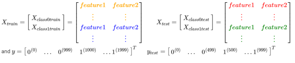
Here we will present gradient descent logistic regression from scratch implemented in Python. We will show a binary classification of two linearly separable datasets. The training set has 2000 examples coming from the first and second class. The test set has 1000 examples, 500 from each class.
First we will import libraries that we need in our code.
Then, we will generate two datasets and plot them.
We will define function which computes the loss function when algorithm predicts \(a \) (\(\hat{y} = a\)),whereas the label for that example is \(y\).
Then, we will define a function to calculate derivatives, it is just one iteration of a previously defined algorithm. The derivative of the loss function with respect to each weigh tells us how loss would change if we modified the parameters.
This is a function for getting optimal values for parmeters \(w\) and \(b \). We will save values of \(w_1, w_2\) and \(b\) so that we can plot them and see how they change through iterations.
We will call iteration_step function for previously defined data set and 1000 iterations.
This is how we will plot values we got from function through_iterations. With following code we will also show how much these parameters and the cost function change .
Last values form list w1_list, w2_list and b_list are the best parameters of logistic regression.
For making predictions with Logistic Regression we need to define sigmoid function.
Code for making predictios is:
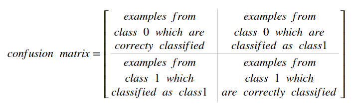
Confusion matrix is a matrix where each row of the matrix represents the instances in a predicted class while each column represents the instances in an actual class (or vice versa). In our case it is \(2×2 \) matrix.
Now we will plot our test before and after classification.
From the confusion matrix we can see that we have 3 misclassified points. To find the complete code for this post, click here.
In the next post we will compare The Implementation of Logistic Regression both from scratch and