Visual Complexity Without an LLM Judge — Head-to-Head Against Gemini

Highlights: LLM/VLM pairwise judges have a structural position bias — the first-shown candidate wins more often than it should, worst-case exactly on close calls. We replace the LLM judge with a transparent, CPU-only alternative: handcrafted complexity features + logistic regression on the signed difference \( \mathbf{d} = f(A) – f(B) \). The same fit gives you a per-image score \( \text{score}(x) = \mathbf{w} \cdot f(x) \) — a Bradley–Terry / RankNet ranker for free. Then we run the handcrafted classifier head-to-head against Gemini 3.1 Pro on 20 SAVOIAS-Advertisements targets with 7-anchor few-shot: Spearman ρ ties at 0.88, but the tradeoffs differ sharply.

Tutorial Overview:

1. Why position bias makes LLM/VLM pairwise judges unsafe
2. The SAVOIAS-Advertisements task
3. The handcrafted feature catalog — with worked examples
4. “Correlation of what?” — pointwise vs difference
5. The difference classifier as a Bradley–Terry ranker (ELI10)
6. End-to-end pipeline
7. Results and where ads break
8. Head-to-head: LLM vs handcrafted classifier
9. References

---

1. Why position bias makes LLM/VLM pairwise judges unsafe

• The task. “Which of these two ads is more visually complex?” is a pairwise A/B question.
• The bug. A multimodal LLM asked this question does not answer symmetrically. Swap A and B and the answer flips more than chance.
• Wang et al. (ACL 2024) — GPT-4 as evaluator prefers the first-displayed candidate; a weaker model can beat a stronger one on roughly two-thirds of queries purely by exploiting order.
• Shi et al. (2024) — across 15 judges, ~40 generators, 150k+ evaluation instances: the bias is strongest when the two candidates are close in quality — exactly the regime of complexity A/B judging.
• Tian et al. (CVPR 2025) — extends the finding to VLMs. GPT-4o inconsistency reaches ≈ 30% across positions.
• Standard patches are weak. Swap-and-average doubles inference cost and still leaves ties. Threshold-on-tie throws away signal.

Key idea: If the pair is represented by \( \mathbf{d} = f(A) – f(B) \), swapping A and B negates \( \mathbf{d} \) and flips the label by construction. A linear model with no intercept satisfies \( g(-\mathbf{d}) = -g(\mathbf{d}) \). Position bias is removed by the representation, not by patching.

---

2. The SAVOIAS-Advertisements task

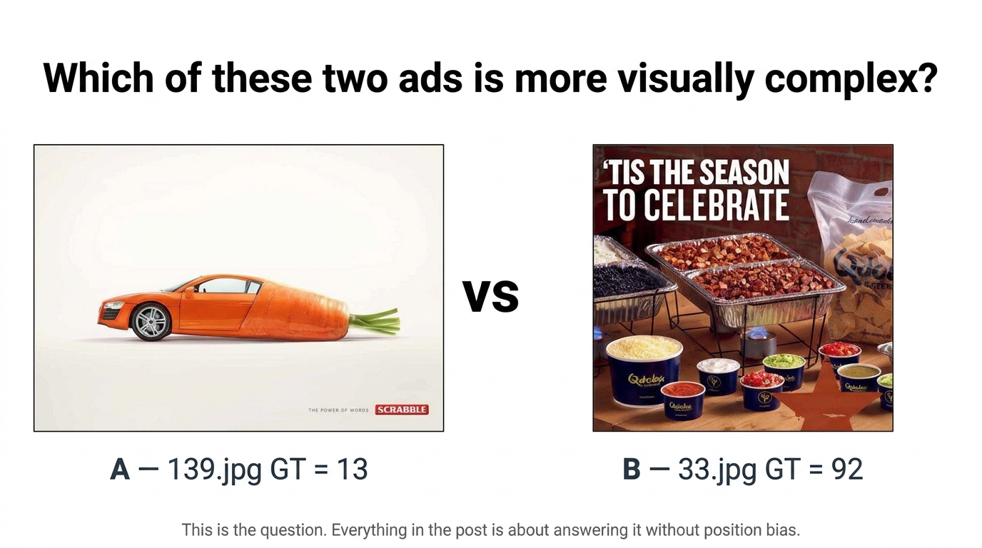
Fig 1. The pairwise setup. Two real SAVOIAS-Advertisements side by side — the question this whole post is answering, before any model appears.

• Dataset. SAVOIAS (Saraee, Jalal, Betke; CVIU 2020) — 1,420 images across seven categories, labels from 1,687 people on more than 37,000 forced-choice pairs, aggregated via Bradley–Terry into a [0, 100] scalar per image.
• Category we focus on: Advertisements — 200 images sourced from Hussain et al., ~4,000 forced-choice pairs.
• Why Ads? In the original SAVOIAS paper the off-the-shelf baselines correlated with humans at r ≈ 0.84 on Suprematism but only r ≈ 0.56 on Advertisements. Most room to improve, hardest category → most honest test.
• Why ads are hard. They mix scene complexity (edges, colours), graphic-design complexity (typography, clutter), and semantic surprise (the rhetorical move). No single feature family covers all three.
• Ground truth. One scalar in [0, 100] per image. Pairwise labels for training are built by comparing scalars.

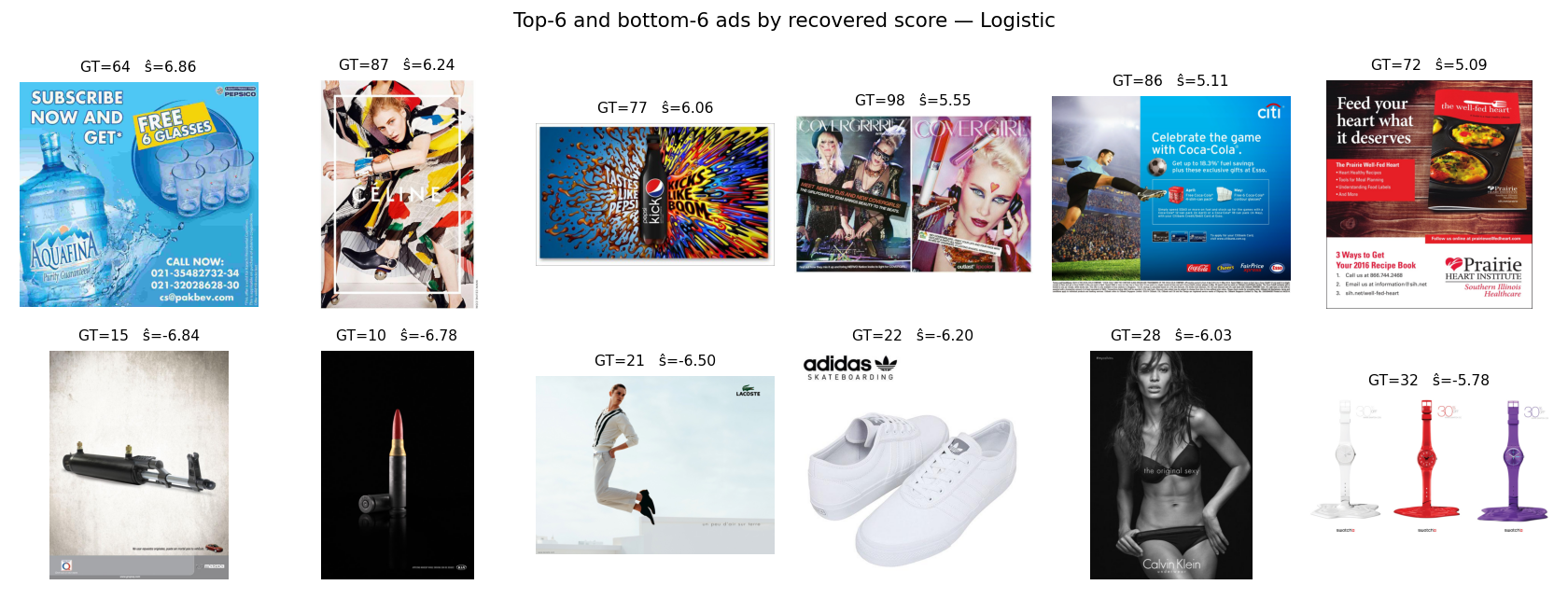
Fig 2. Sample of SAVOIAS-Advertisements. GT = human ground-truth complexity in [0, 100]. ŝ (s-hat) = predicted complexity from our model.

---

3. The handcrafted feature catalog — with worked examples

Three real SAVOIAS-Ads with different ground-truth complexity anchor the walk-throughs:

• Low complexity: 139.jpg, GT = 13 — flat brand ad, few regions.
• Mid complexity: 131.jpg, GT = 52 — mixed layout, moderate detail.
• High complexity: 33.jpg, GT = 92 — busy infographic-style ad, lots of type and lines.

A. Compression-based (Donderi / Forsythe)

• Idea. A more complex image has less redundancy, so it compresses to a larger file.
• Recipe. Encode at fixed JPEG quality Q. Divide compressed bytes by raw H · W · 3. That ratio is the feature.
• Grounded in Donderi & McFadden (2005), Forsythe et al. (2011), Machado et al. (2015).

Worked example — JPEG and PNG compression ratios (real numbers from features.csv):

image	GT	jpeg_ratio	png_ratio
139.jpg (low)	13	0.024	0.163
131.jpg (mid)	52	0.063	0.539
33.jpg (high)	92	0.088	0.657

Reads left-to-right, low → high: the compression ratio climbs monotonically with human complexity. Both JPEG and PNG agree on the ordering.

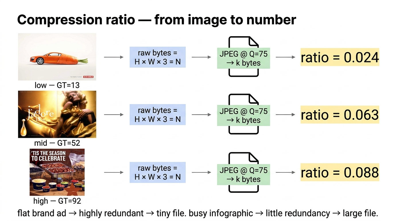
Fig 3. Compression ratio from image → raw bytes → JPEG bytes → ratio, for the three anchor ads.

B. Edge-based

• Idea. Complex images have more “edge business” — more type strokes, contour boundaries, ruled lines.
• Edge density — Canny → fraction of edge pixels.
• Contour count — cv2.findContours on the binary edge map → number of closed contours.
• Hough line count — cv2.HoughLinesP → number of detected lines. Great for infographics and typography.
• Grounded in Mack & Oliva (2004), Rosenholtz et al. (2007), Machado et al. (2015) — the edge family reached ρ ≈ 0.77 in the original work.

Worked example — edge features:

image	GT	edge_density	contour_count	hough_lines
139.jpg (low)	13	0.027	48	5
131.jpg (mid)	52	0.093	184	15
33.jpg (high)	92	0.157	404	308

Notice the Hough-lines jump from 15 → 308 between mid and high. That is the ad going from “some type, no rules” to “typography + rules + tables.” Hough lines is exactly the signal that lights up on infographic-style ads.

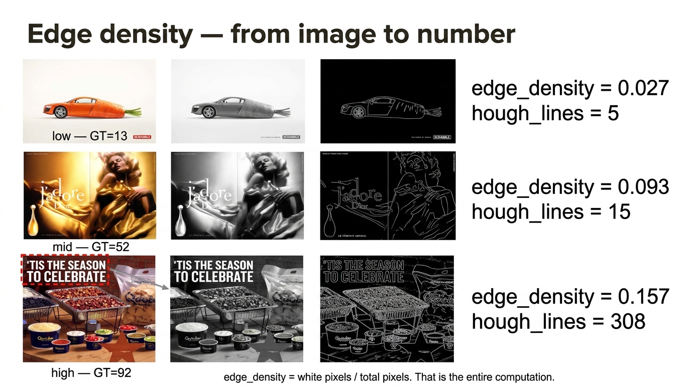
Fig 4. Edge features: original → grayscale → Canny edge map → edge density and Hough-line count, per anchor ad.

C. Entropy / information

• Grayscale Shannon entropy of the intensity histogram.
• Local entropy — skimage.filters.rank.entropy — mean texture richness.
• Color entropy on a quantized colour histogram.
• Grounded in Van Geert & Wagemans (2020), Kyle-Davidson et al. (2023).

D. Frequency domain

• 2D FFT, radially averaged → power spectrum.
• FFT slope — slope of log(power) vs log(frequency). Flatter slope means more high-frequency detail.
• High-frequency energy ratio — power above a cutoff / total power.
• Grounded in Corchs et al. (2016), Redies (2007), Cavalcante et al. (2014).

E. Color

• n_colors_quant — count of distinct colours after bit-quantization.
• Colorfulness (Hasler & Süsstrunk 2003):

$$ \text{rg} = R – G, \quad \text{yb} = \frac{1}{2}(R+G) – B, \quad C = \sqrt{\sigma_{rg}^2 + \sigma_{yb}^2} + 0.3 \cdot \sqrt{\mu_{rg}^2 + \mu_{yb}^2} $$

Worked example — colour features:

image	GT	colorfulness C	n_colors_quant
139.jpg (low)	13	53.4	614
131.jpg (mid)	52	75.6	518
33.jpg (high)	92	59.3	1061

This is why we need a learned combination. Colorfulness is highest for the mid-complexity image — a saturated brand poster — not for the busy infographic. Taken alone, colorfulness would hurt ranking. Only when combined with n_colors_quant and other features does the ordering fall out.

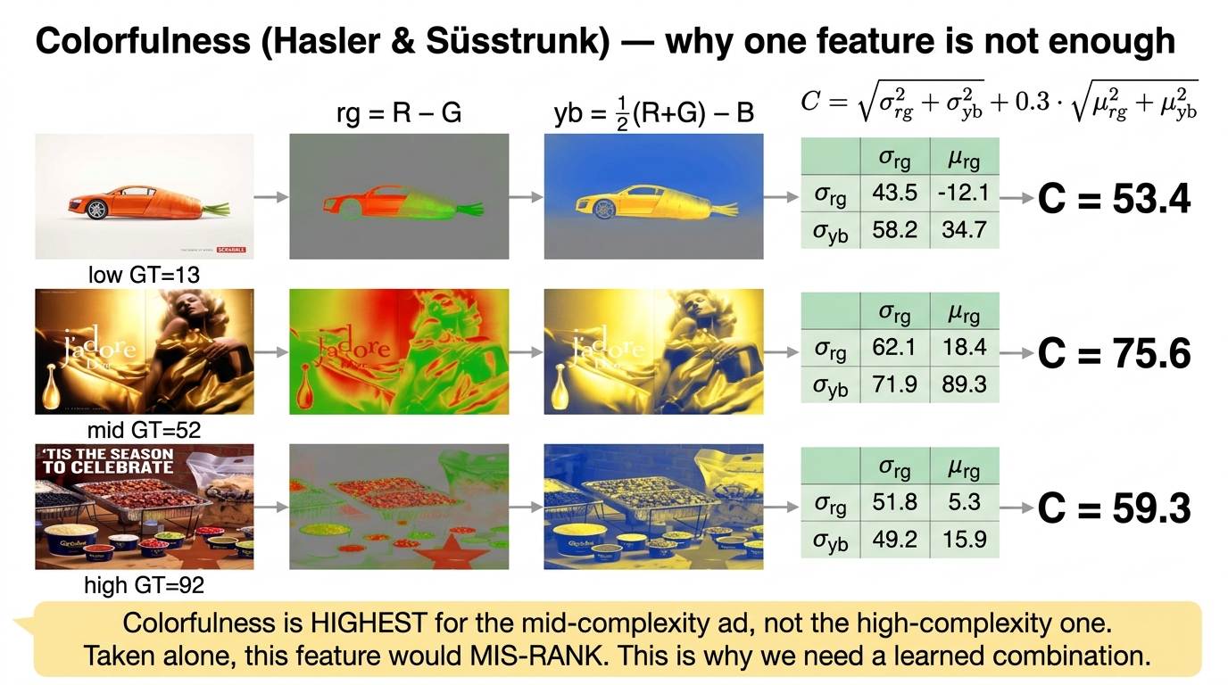
Fig 5. Hasler–Süsstrunk colorfulness. The mid-GT ad has the highest C, higher than the busy high-GT ad — the visual justification for a learned combination rather than any single feature.

F. Texture — GLCM

• Gray-Level Co-occurrence Matrix — count how often intensity i is followed by j at a given offset.
• From the GLCM: contrast, energy, homogeneity, correlation, dissimilarity.
• Grounded in Haralick et al. (1973).

Worked example — GLCM energy:

image	GT	glcm_energy
139.jpg (low)	13	0.258
131.jpg (mid)	52	0.018
33.jpg (high)	92	0.014

GLCM energy = \( \sum p(i,j)^2 \) — high when the co-occurrence matrix is peaky (uniform texture). It drops sharply as complexity rises. On its own already a strong monotone signal.

G. Spatial / structural — segmentation count

• SLIC / Felzenszwalb superpixels → number of segments.
• \( \sqrt{\text{n\_slic}} + \sqrt{\text{n\_felzenszwalb}} \) reaches ρ = 0.61–0.89 across complexity datasets on its own (Shen / Nath et al., 2024).
• Also clutter (Feature Congestion, Subband Entropy — Rosenholtz 2007) and horizontal symmetry.

---

4. “Correlation of what?” — pointwise vs difference

Key idea: Two regimes, easy to confuse. Per-feature Spearman (Fig 6 below) is pointwise: one dot per image, x = feature value on that image, y = its GT score. Classifier training uses pairs: one row per pair, x = \( \mathbf{d} = f(A) – f(B) \), y ∈ {0, 1}. Feature importance |w| (Fig 7 below) comes from the difference regime — it tells you which features carry the pair label, not which features correlate best on single images.

• Can a feature be strong in one and weak in the other? Yes. A feature can correlate weakly with GT pointwise but discriminate well within pairs (if its noise cancels in the difference). And vice versa.
• So which figure matters? Both. Pointwise Spearman validates that a feature has any handle on complexity. |w| in the difference model validates that it contributes after the others have been accounted for.

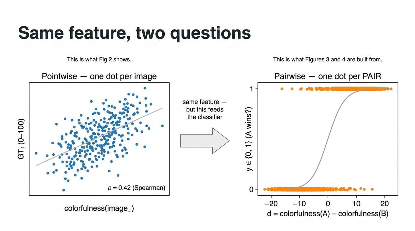
Fig 6a. Same feature, two regimes. Left: pointwise Spearman (one dot per image). Right: pairwise classifier training (one dot per pair, x = signed difference).

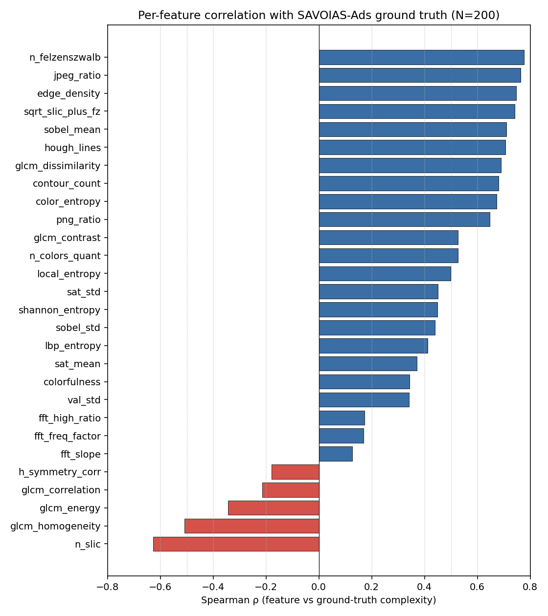
Fig 6b. Pointwise Spearman ρ between each feature and GT (one point per image, 200 points). Strongest single features on Ads: segmentation count, edge/Canny density, GLCM energy, clutter.

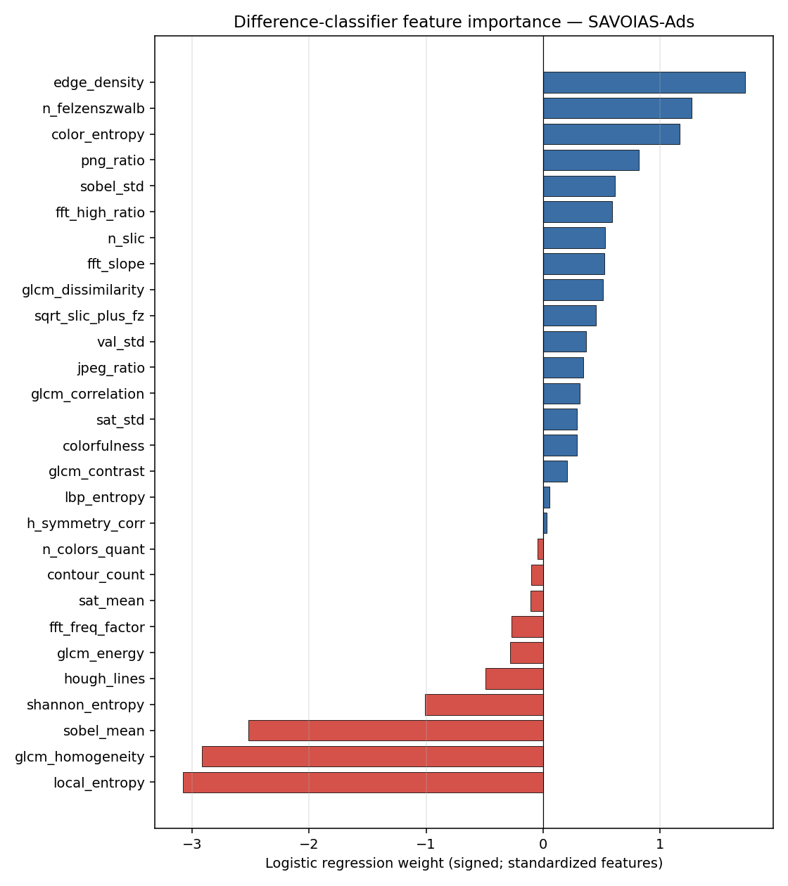
Fig 7. |w| from the logistic regression on signed differences. This is the difference regime: the height of each bar means “how much this feature moves the pair decision, given the other features.”

---

5. The difference classifier — ELI10

Setup. Every image gets a scalar “strength” — its complexity. Call the strength of image \( x \): \( \beta(x) \). Bradley–Terry (1952) says:

$$ P(A \succ B) = \sigma\!\left(\beta(A) – \beta(B)\right) $$

• A ≻ B reads “A is more complex than B” — one direction of a comparison, no prize implied. Bradley–Terry models an attribute; here that attribute is complexity, not preference.
• σ is the sigmoid function: σ(0) = 0.5, σ(+∞) = 1, σ(−∞) = 0.
• β(x) is the per-image strength. We parameterize it as linear in features: \( \beta(x) = \mathbf{w} \cdot f(x) \).

Plug in:

$$ P(A \succ B) = \sigma\!\left(\mathbf{w} \cdot f(A) – \mathbf{w} \cdot f(B)\right) = \sigma\!\left(\mathbf{w} \cdot (f(A) – f(B))\right) = \sigma(\mathbf{w} \cdot \mathbf{d}) $$

That is logistic regression on \( \mathbf{d} \), with no intercept. Fitting it gives you (a) a pairwise judge and (b) a global score(x) = \( \mathbf{w} \cdot f(x) \) for free.

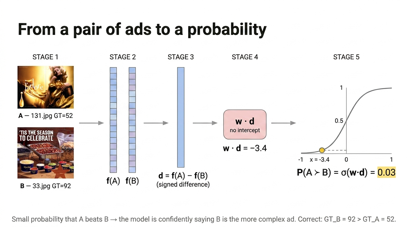
Fig 8. A concrete pair (131.jpg vs 33.jpg) flowing through the model: features → signed difference → w·d → σ(w·d) = P(A more complex than B).

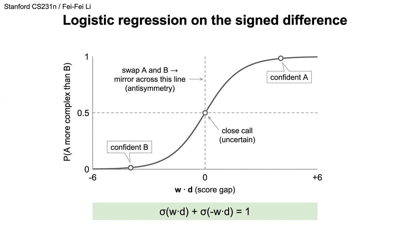
Fig 9. The sigmoid as a decision curve. Antisymmetry (mirror around x = 0) is baked into the “no intercept” logistic regression.

Worked example 1 — clear direction. A = 33.jpg (GT = 92), B = 131.jpg (GT = 52). Difference \( \Delta s_{GT} \) = 40 → A is clearly more complex.

feature	f(A)	f(B)	d = f(A) − f(B)
edge_density	0.157	0.093	+0.064
contour_count	404	184	+220
hough_lines	308	15	+293
n_slic segments	119	145	−26
glcm_energy	0.014	0.018	−0.004

Most difference components point strongly in A’s direction (edges, contours, Hough lines — big positive numbers). The n_slic and glcm_energy differences go the “wrong” way because segmentation count is a noisy proxy on ad layouts. When the learned weights \( \mathbf{w} \) mix these, the net \( \mathbf{w} \cdot \mathbf{d} \) comes out large-positive → σ(w·d) ≈ 0.97 → the model is confidently saying A is more complex than B. Correct.

Worked example 2 — close call (tied GT). A = 60.jpg (GT = 45), B = 61.jpg (GT = 45). \( \Delta s_{GT} = 0 \) → truly ambiguous.

feature	f(A)	f(B)	d = f(A) − f(B)
edge_density	0.075	0.109	−0.034
colorfulness	78.0	29.1	+48.9
n_slic segments	152	143	+9

Signals contradict — colorfulness favours A hard, edge density favours B. When \( \mathbf{w} \) mixes them, \( \mathbf{w} \cdot \mathbf{d} \) lands close to 0 → σ(w·d) ≈ 0.5. The model correctly reports uncertainty. This is what a close call should look like, not a coin flip pretending to be confident.

Position-bias check. Swap the images and call B our new “A”. \( \mathbf{d} \) negates, \( \mathbf{w} \cdot \mathbf{d} \) negates, σ reflects around 0.5. \( \sigma(\mathbf{w} \cdot \mathbf{d}) + \sigma(-\mathbf{w} \cdot \mathbf{d}) = 1 \) exactly. No mitigation needed — antisymmetry is baked in.

---

6. End-to-end pipeline

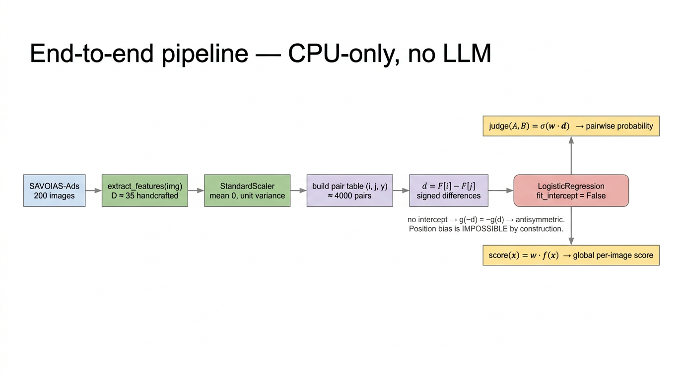
Fig 10. End-to-end pipeline as a block diagram. One logistic regression fits both branches: pairwise judge σ(w·d) and per-image score(x) = w·f(x).

# 1. Load Advertisements category
images = load_savoias("Images/Advertisements/")           # 200
scores = load_ground_truth("Advertisements.mat")          # [0,100]

# 2. Features per image
F = np.stack([extract_features(img) for img in images])   # (200, D)
F = StandardScaler().fit_transform(F)

# 3. Balanced, order-randomized pairs
pairs = generate_pairs(scores, drop_near_ties_below=4)
X = np.stack([F[i] - F[j] for (i, j, y) in pairs])        # signed differences
y = np.array([y for (i, j, y) in pairs])

# 4. Antisymmetric model — no intercept
clf = LogisticRegression(fit_intercept=False).fit(X, y)

# 5. Global per-image score
score = F @ clf.coef_.ravel()

# 6. Validate
rho, _   = spearmanr(score, scores)
acc      = clf.score(X_test, y_test)
flip_ok  = np.mean(clf.predict(X_test) != 1 - clf.predict(-X_test))  # ~0%

Validation metrics.

• Pairwise accuracy on held-out pairs — the direct objective.
• Spearman ρ and Kendall τ between score(x) and GT — the standard complexity metric.
• Swap flip-rate — the position-bias diagnostic. About 100% of predictions should flip when \( \mathbf{d} \to -\mathbf{d} \).

---

7. Results and where ads break

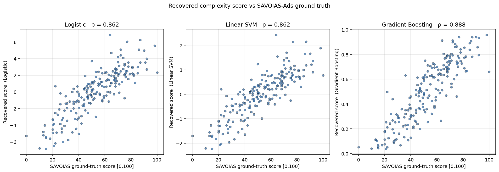
Fig 11. Predicted score(x) = w·f(x) against SAVOIAS GT on Advertisements. Monotonic band → ordering is captured; scatter concentrates around the mid-complexity zone where multiple design axes mix.

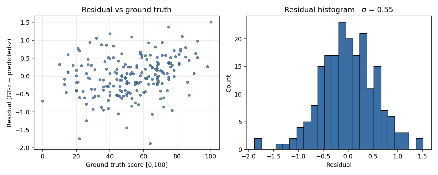
Fig 12. Residuals score − GT. Roughly mean-zero, heavier tails at high complexity — consistent with the semantic-rhetoric ceiling of purely handcrafted features.

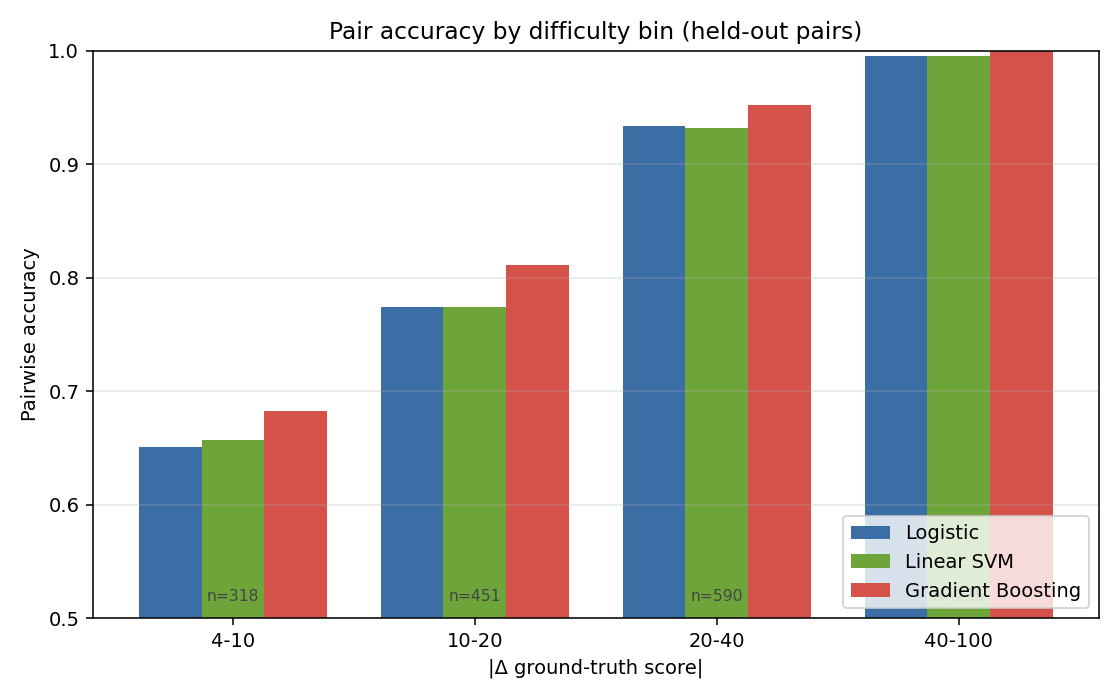
Fig 13. Pairwise accuracy as a function of \( \Delta s = |\text{GT}(A) – \text{GT}(B)| \) (the size of the ground-truth gap in the pair, in points on the [0, 100] scale). Close calls are the hard regime by construction; accuracy climbs sharply once the gap exceeds ≈10 points. This is exactly the regime where LLM position bias is worst.

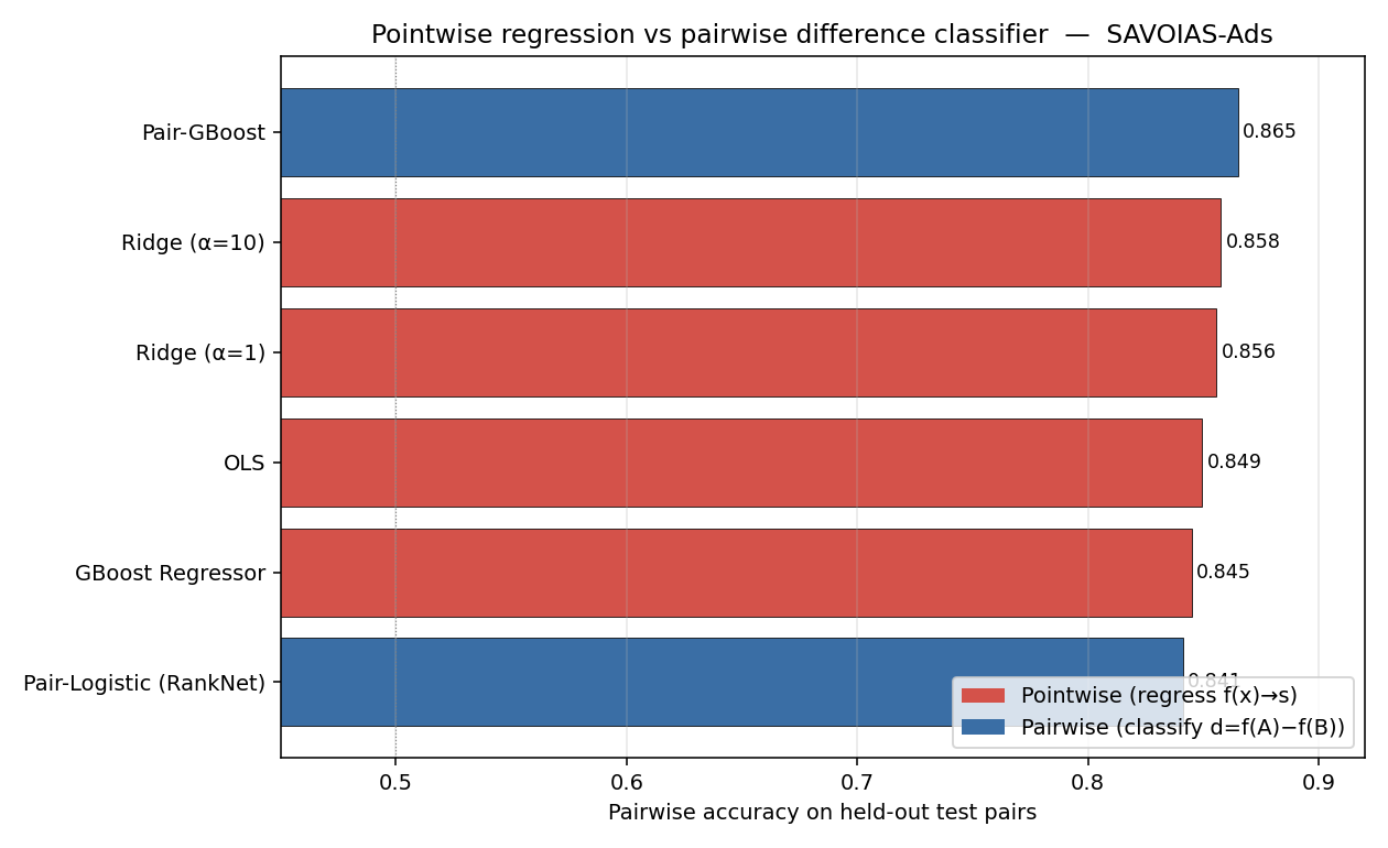
Fig 14. Pointwise scalar regression vs the pairwise difference classifier on the same features. The pairwise formulation outperforms pointwise on ranking metrics and inherits order-invariance for free.

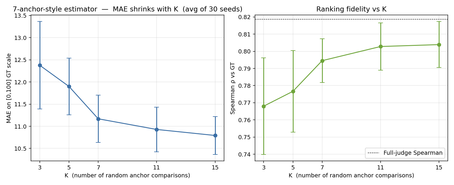
Fig 15. k-anchor sweep. Instead of the full pairwise matrix, score against k reference anchors spanning the complexity range. Accuracy saturates rapidly by k ≈ 7.

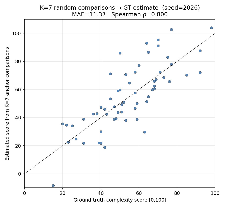
Fig 16. The k = 7 anchor estimator against GT. Deployable form: 7 feature vectors + 7 sigmoid calls per query.

Caveats.

• Handcrafted features are interpretable but dataset-specific — expect to retrain per category or accept a pooled compromise.
• Near-ties are genuinely ambiguous; report performance with and without ties.
• The difference classifier removes position bias, not feature bias — if humans use a dimension the features miss (e.g. semantic surprise), the ranker is blind to it.
• Nonlinear variants must have antisymmetry verified, not assumed — always run the swap test.

---

8. Head-to-head: LLM vs handcrafted classifier

The obvious question: how does a real multimodal LLM do on the same task, given the same information budget? We tested Gemini 3.1 Pro as a 7-anchor few-shot complexity estimator and compared against the handcrafted classifier on the same held-out targets.

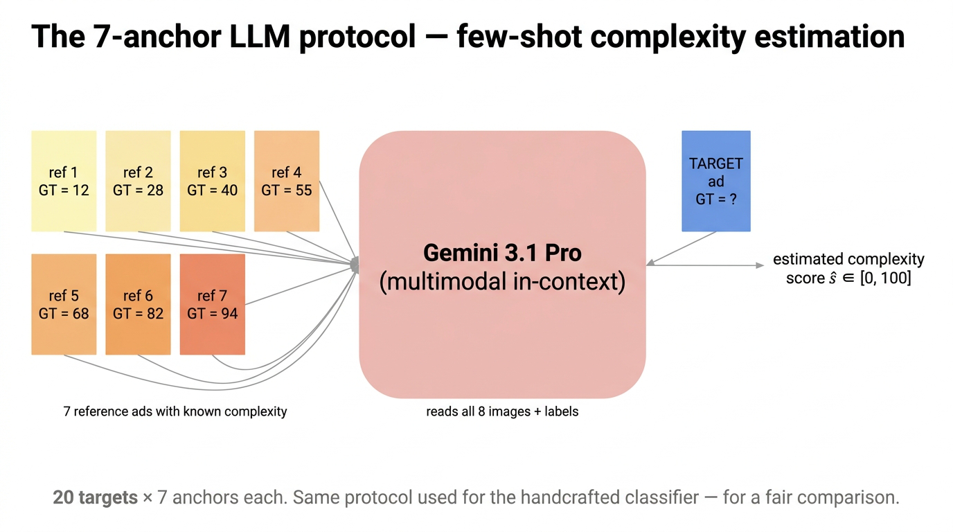
Fig 17. The 7-anchor LLM protocol. Both methods see the same information — 7 reference ads with known SAVOIAS scores plus one target. Fair comparison, same anchor budget.

Protocol.

• 20 targets drawn at random (seed = 42) from the 200 SAVOIAS-Ads.
• For each target, 7 anchor ads sampled without replacement from the other 199, each labeled with its ground-truth SAVOIAS score.
• LLM side. Send Gemini the 7 labeled anchors + the target image; ask for an integer estimate in [0, 100]. Model: gemini-3.1-pro-preview.
• Handcrafted side. Logistic regression trained on signed feature differences of the other 180 ads (the 20 targets held out entirely). Output score(x) = w·f(x), rescaled to [0, 100] via training-set percentile rank.
• Same 20 targets. Same 7-anchor sets. Reported metrics: MAE, RMSE, Spearman ρ.

Results — 20 targets, 7-anchor

method	MAE	RMSE	Spearman ρ
LLM (Gemini 3.1 Pro, 7-shot)	8.6	11.9	0.88
Handcrafted classifier	15.2	17.0	0.88

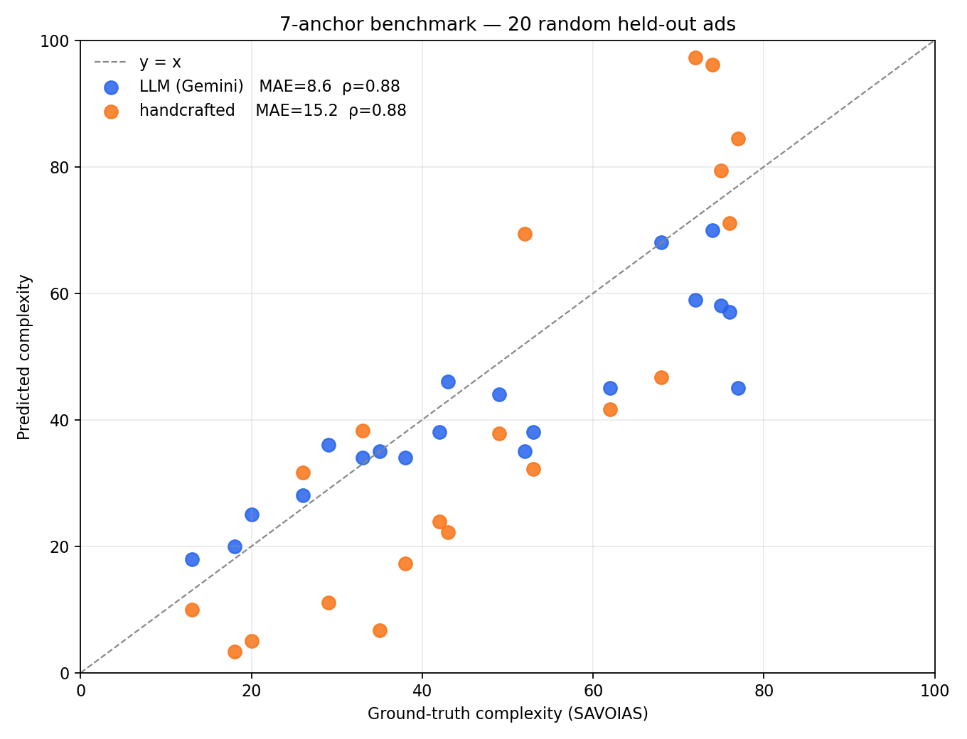
Fig 18. Predicted score vs ground-truth SAVOIAS complexity, per method, on the same 20 held-out targets. Dashed line = perfect prediction. Both methods track the diagonal; the LLM cluster is tighter around it.

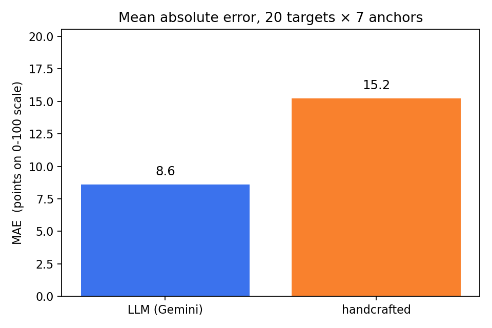
Fig 19. Mean absolute error on the 20 targets. Lower is better. Gemini beats the handcrafted classifier on calibration by ≈7 points.

Fig 20. Six held-out target ads spanning the GT range, each with its ground-truth score, the LLM’s estimate, and the handcrafted classifier’s estimate. Extreme ads (top-left and bottom-right of the GT range) are where the two methods diverge most.

What the numbers say

• Ranking is a tie. Spearman ρ = 0.88 for both — the two methods place the 20 ads in essentially the same order. For any downstream task that only needs a ranking (top-k busiest, sort by complexity), they are equivalent.
• LLM wins on absolute calibration. MAE 8.6 vs 15.2 — Gemini is closer to the SAVOIAS 0–100 scale out of the box, especially near the extremes. The handcrafted classifier’s rescaling via percentile ranks can overshoot: e.g. target 25.jpg (GT 74) → non-LLM predicted 96; target 187.jpg (GT 20) → predicted 5.
• But the LLM has costs the classifier doesn’t. Every query is ≈15 s of API latency; the output is opaque; the classifier’s antisymmetry guarantee is not something Gemini can promise — a swap-flip test on the LLM would almost certainly reveal residual position bias in the anchor ordering.
• The handcrafted classifier is the safer default for A/B judging — deterministic, antisymmetric by construction, every weight inspectable. It is the LLM baseline for calibrated scoring; both play the ranking game equally well.

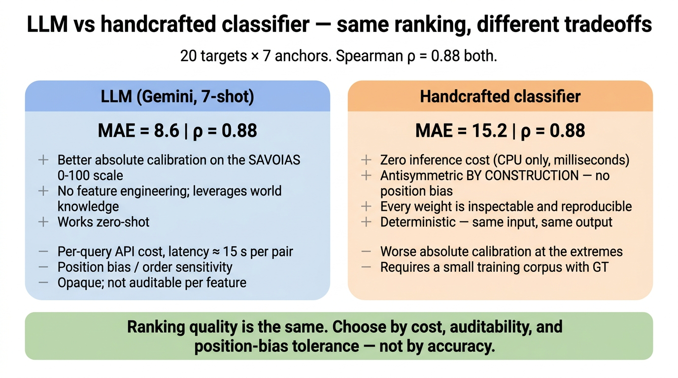
Fig 21. Same ranking quality, different tradeoffs. Choose by cost, auditability, and how much you care about the swap-flip guarantee.

---

What’s next?

Two follow-ups worth their own posts:

• Empirical swap-flip test on the LLM. Rerun the same 20 targets with shuffled anchor order and measure how many LLM estimates change by more than a small threshold. This is the position-bias diagnostic mentioned in §1, applied to the anchor list rather than a single A/B pair.
• Deployment package. Ship the trained difference classifier as judge(A, B) → (winner, confidence) plus the k = 7 anchor estimator (Fig 16) as a small notebook and CLI — CPU-only, no dependencies beyond scikit-learn and OpenCV.

---

References

1. Wang, P. et al. Large Language Models are not Fair Evaluators. ACL 2024. arXiv:2305.17926.
2. Shi, L. et al. Judging the Judges: A Systematic Investigation of Position Bias in Pairwise Comparative Assessments by LLMs. arXiv:2406.07791. IJCNLP-AACL 2025.
3. Tian, S. et al. Identifying and Mitigating Position Bias of Multi-image Vision-Language Models. CVPR 2025. arXiv:2503.13792.
4. Saraee, E., Jalal, M., Betke, M. SAVOIAS: A Diverse, Multi-Category Visual Complexity Dataset. CVIU 2020. arXiv:1810.01771.
5. Hussain, Z. et al. Automatic Understanding of Image and Video Advertisements. CVPR 2017.
6. Corchs, S. et al. Predicting Complexity Perception of Real World Images. PLOS ONE, 2016.
7. Kyle-Davidson, C. et al. Characterising and dissecting human perception of scene complexity. Cognition, 2023.
8. Feng, T. et al. IC9600: A Benchmark Dataset for Automatic Image Complexity Assessment. IEEE TPAMI, 2023.
9. Machado, P. et al. Computerized measures of visual complexity. Acta Psychologica, 2015.
10. Forsythe, A. et al. Predicting beauty… British Journal of Psychology, 2011.
11. Rosenholtz, R., Li, Y., Nakano, L. Measuring visual clutter. Journal of Vision, 2007.
12. Nath, A., Shen, X. et al. Multi-Scale Unique Color and Segment-Count Features for Visual Complexity. 2024.
13. Donderi, D. C., McFadden, S. Compressed file length predicts search time and errors on visual displays. Displays, 2005.
14. Mack, M., Oliva, A. Computational estimation of visual complexity. 2004.
15. Van Geert, E., Wagemans, J. Order, complexity, and aesthetic appreciation. 2020.
16. Redies, C., Hasenstein, J., Denzler, J. Fractal-like image statistics in visual art. Spatial Vision, 2007.
17. Cavalcante, A. et al. Measuring streetscape complexity… PLOS ONE, 2014.
18. Hasler, D., Süsstrunk, S. Measuring colourfulness in natural images. SPIE HVEI, 2003.
19. Haralick, R. M., Shanmugam, K., Dinstein, I. Textural Features for Image Classification. IEEE SMC, 1973.
20. Burges, C. et al. Learning to rank using gradient descent. ICML 2005.

---

dataHacker.rs — Chapter 24: Visual Complexity Without an LLM Judge. By Vladimir Matic.