Highlights: An image is just a matrix — but the Transformer eats sequences of vectors. The whole “vision” trick of ViT lives in how that matrix is turned into a sequence. We cut a 224×224 image into a fixed 14×14 grid of 16×16 patches, flatten each, and project it through ONE learned Linear layer. Patches are not sampled — every cell of the grid becomes a token, in fixed order. We prepend a learnable [CLS] token, add a learnable position embedding, and reach a [197, 768] matrix that an ordinary 12-block Transformer encoder consumes. Out the other end we slice the CLS row — a single 768-dim vector that IS the image embedding, exactly like CLIP. By the end of the post we run real pretrained vit_base_patch16_224 weights from timm on a photo with no training and no API, then prove the [768] vector knows shape by separating circles from squares with 100% linear-probe accuracy and a single PCA component.

Stack: PyTorch  |  timm (HuggingFace Hub)  |  scikit-learn for the linear probe  |  matplotlib for figures. No GPU required.

Stat badges: 86.6M Parameters  |  197 Tokens  |  768 Embedding Dim  |  12 Layers  |  12 Heads  |  100% Probe Accuracy  |  $0 GPU Cost

Tutorial Overview

1. The 224×224 input image — and why the number 224
2. From image to patches — the fixed 14×14 grid
3. The linear projection — the image “tokenizer”
4. The [CLS] token — one vector, shared across every image
5. Position embeddings — restoring 2D geometry
6. The [197, 768] sequence — where shapes finally settle
7. What B is, and what comes OUT of the Transformer
8. The explicit version — same math, no Conv2d
9. What happens inside the encoder — Q/K/V, multi-head, residual stream
10. A minimal Vision Transformer — runnable in one cell
11. Real pretrained weights — classification + linear probe (no API)
12. What lives in the [768] vector? — circles vs squares, an honest probe
13. Summary and what’s next

---

1. The 224×224 input image

A Vision Transformer takes one RGB image at 224×224 — three channels, 224 tall, 224 wide. In PyTorch it carries a batch dimension first: [B, 3, 224, 224].

Why 224? Two reasons stacked on one number. First, it is the ImageNet resolution all the pretrained weights expect, so a hand-built ViT can load them unchanged. Second, 224 / 16 = 14 — the image tiles into a clean 14 × 14 grid of 16×16 patches with nothing left over.

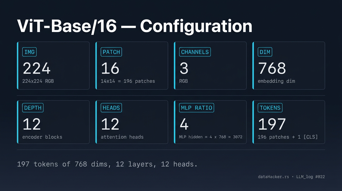
Fig 1. ViT-Base/16 — every number you need on one card. These exact values match the pretrained timm checkpoint, which is why our hand-built model can load real ViT weights unchanged.

One sentence summary of everything in the card: 197 tokens of 768 dims, 12 layers, 12 heads — and that is the whole model.

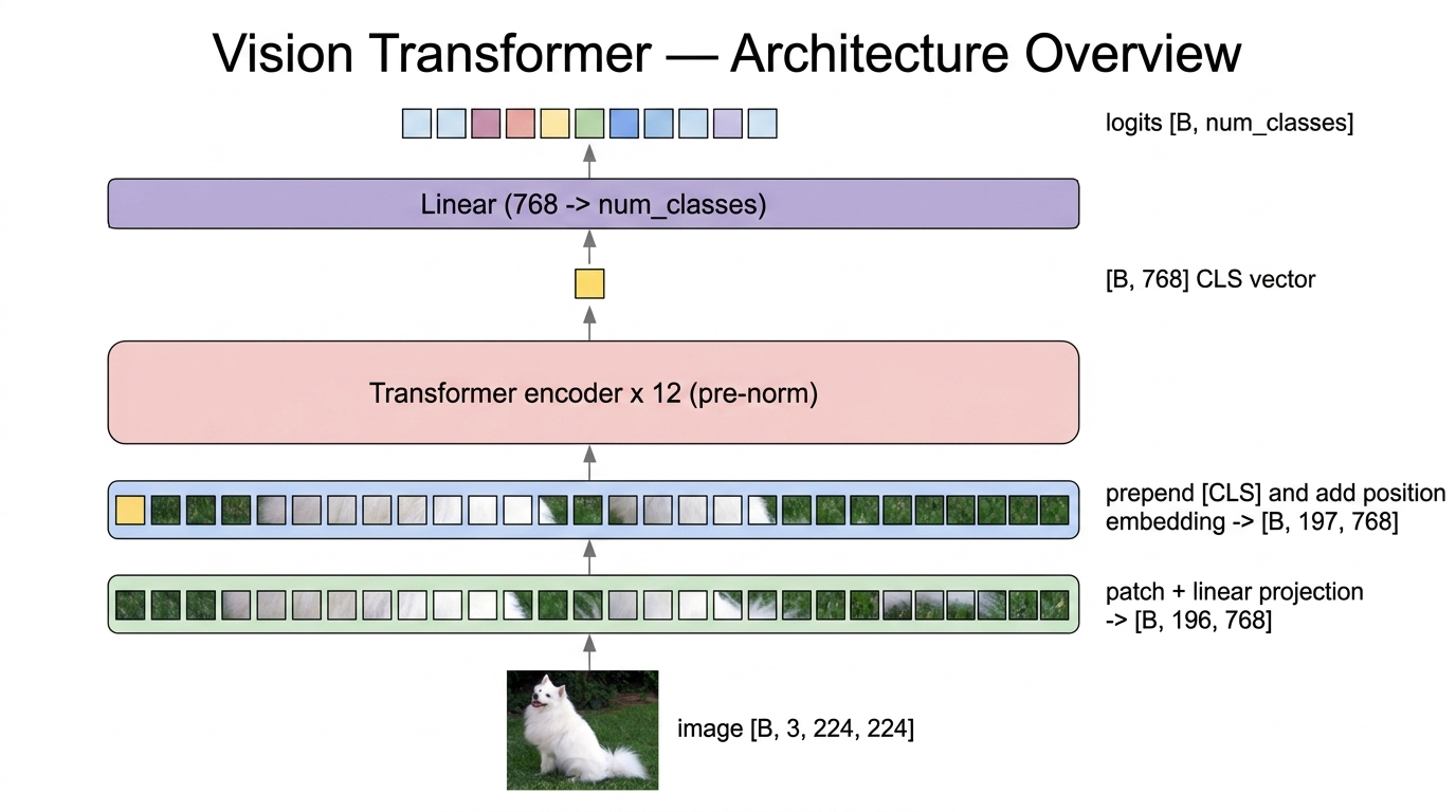
Fig 2. ViT-Base/16 end to end. Image → patch + linear projection → CLS prepended + position embedding added → 12 encoder blocks → final LayerNorm → take CLS → linear classification head → logits. The token count flips from 196 to 197 once and never changes again; the embedding dim stays 768 everywhere.

2. From image to patches — the fixed 14×14 grid

We cut the image into squares of 16×16 pixels. Since 224 / 16 = 14, the image becomes a 14 × 14 grid → 196 patches.

Say it once and never confuse it again: the patch is 16×16 pixels; 14×14 is the grid — the number of patches across and down, not their size. Each patch holds 16 × 16 × 3 = 768 raw pixel values when flattened.

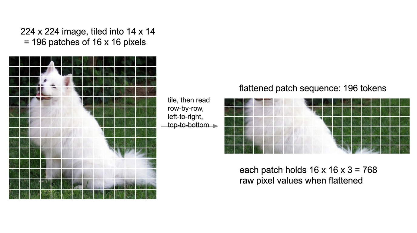
Fig 3. The 224×224 image is tiled with the fixed 14×14 grid and read row by row into a 196-token sequence. Each patch holds 16 × 16 × 3 = 768 raw pixel values when flattened.

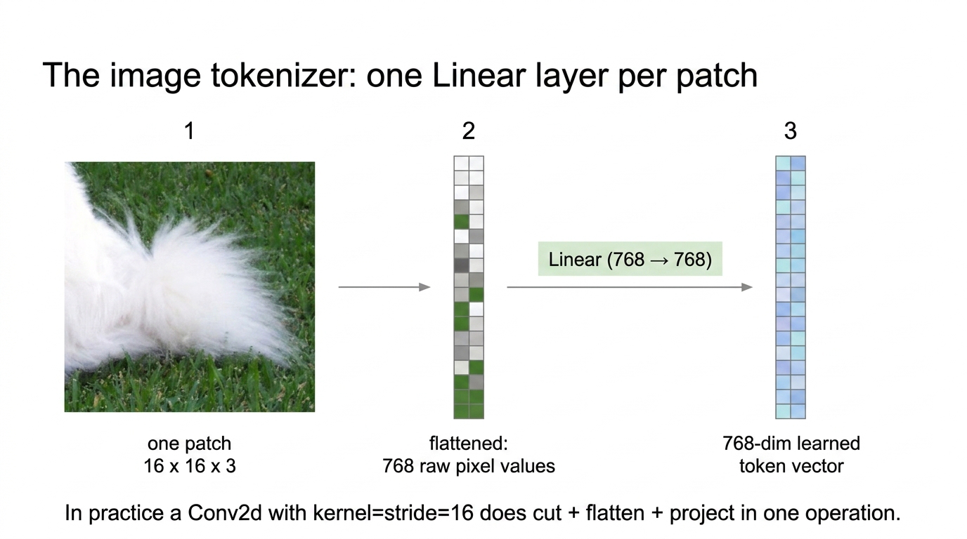
3. The linear projection — the image “tokenizer”

A flattened patch is 768 raw pixel numbers. We pass it through one learnable Linear(768 → 768), turning raw pixels into a learned representation. For all 196 patches we get a [196, 768] matrix — one learned token per patch.

This single linear layer is the image tokenizer. Text models look up an embedding from a vocabulary table; an image has no vocabulary, so this learned projection IS the tokenizer. There is no dictionary anywhere in ViT.

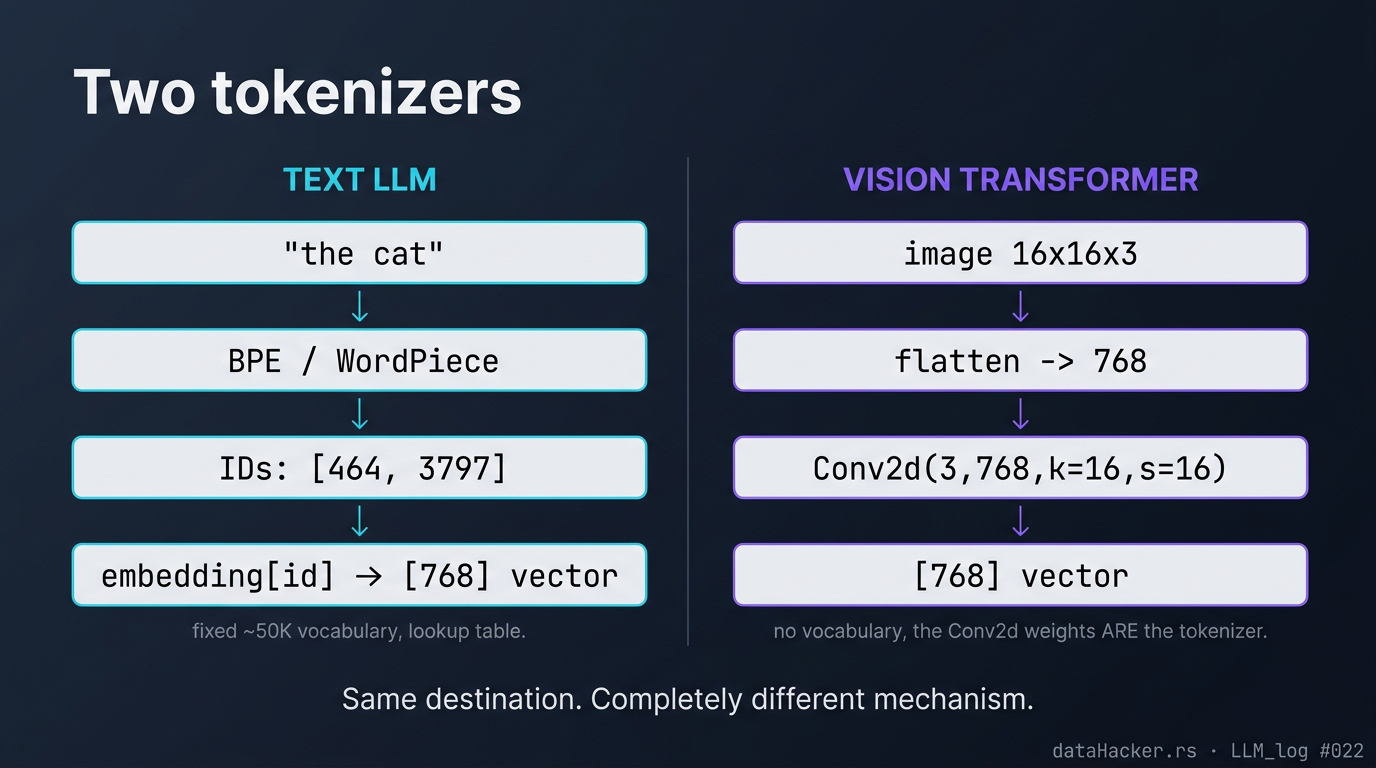
Fig 4. Two tokenizers. A text LLM looks an ID up in a ~50K-row vocabulary; ViT projects raw pixels with one Conv2d. Same destination (a 768-vector), completely different mechanism.

One subtlety: 16 × 16 × 3 = 768 equals D = 768 only because this is ViT-Base/16, so the projection looks square. For ViT-Tiny (D = 192) it would be Linear(768 → 192). The flatten size and the embedding dim are independent — they happen to match here.

In practice we use a single Conv2d with kernel = stride = patch size, which does cut + flatten + project in one operation:

# !pip install torch
import torch
import torch.nn as nn
B, C, IMG, P, D = 1, 3, 224, 16, 768
x = torch.randn(B, C, IMG, IMG)              # [1, 3, 224, 224]
patch_embed = nn.Conv2d(C, D, kernel_size=P, stride=P)
out = patch_embed(x)         # [1, 768, 14, 14]  one 768-vector per grid cell
out = out.flatten(2)         # [1, 768, 196]     flatten the 14x14 grid into 196
patches = out.transpose(1, 2) # [1, 196, 768]  put patches first, dims last
print(patches.shape)         # torch.Size([1, 196, 768])

The Conv2d with no overlap (stride equals kernel) is mathematically identical to “flatten each patch and apply Linear(768, 768)”. It is not a CNN-style spatial convolution; it is just an efficient way to do the same projection 196 times.

Fig 5. One patch goes through three operations: cut (16×16×3 pixels) → flatten (768-vector of raw pixels) → project (Linear(768 → 768)) → 768-dim learned token. Repeat 196 times.

4. The [CLS] token — one vector, shared across every image

We prepend one extra vector: the classification token, [CLS]. It is a single learnable vector of length 768 — an nn.Parameter of shape [1, 1, 768]. It is not computed from the image; the model trains it.

Prepending it gives 196 + 1 = 197 tokens. After the 12 encoder blocks, this one token will have attended to every patch in every layer, so we read the classification answer off it.

cls = nn.Parameter(torch.zeros(1, 1, D))     # [1, 1, 768] the learnable CLS
cls = cls.expand(B, -1, -1)                   # copy per image -> [B, 1, 768]
sequence = torch.cat([cls, patches], dim=1)   # prepend -> [B, 197, 768]
print(sequence.shape)                         # torch.Size([1, 197, 768])

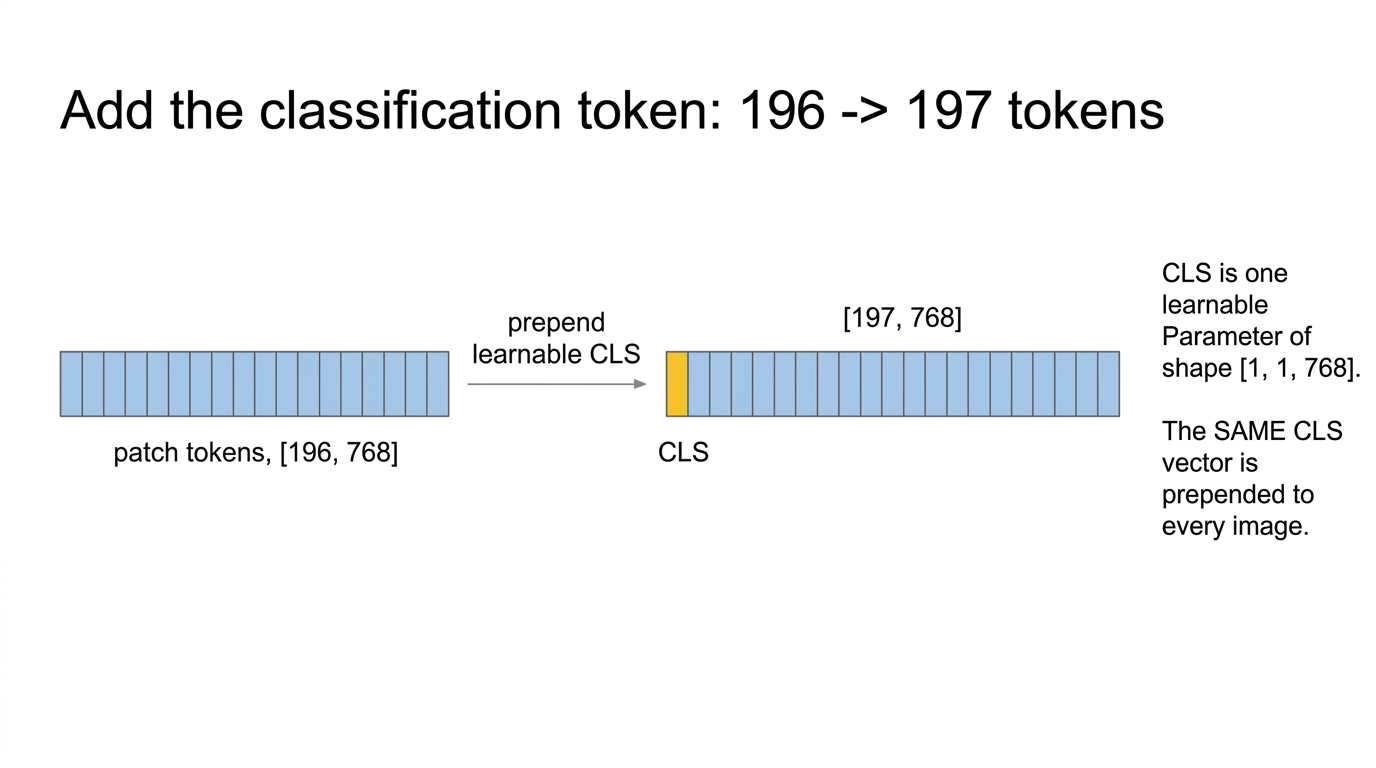
Fig 6. Prepending the [CLS] vector flips the token count from 196 to 197. The embedding dim stays at 768.

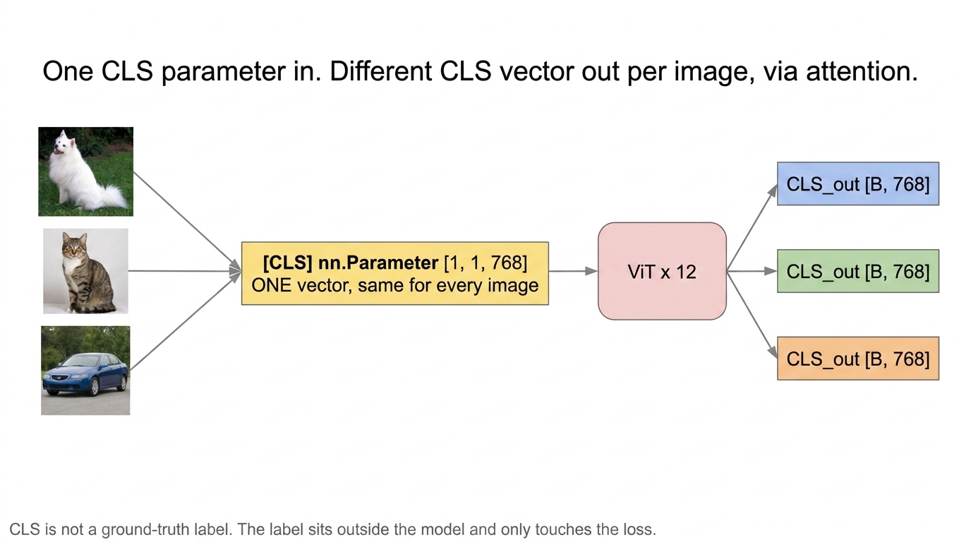
Fig 7. One CLS parameter in (yellow), three different CLS outputs out. The difference is built up by 12 layers of attention with each image’s patches — not by any per-image CLS input.

5. Position embeddings — restoring 2D geometry

Patches carry no built-in order — once we have the matrix [196, 768], the Transformer does not know patch 5 sat above patch 19. So we add a learnable position embedding: a table of shape [1, 197, 768], one 768-vector per position, added element-wise to the tokens. One row for the CLS position, 196 for the patches.

It is just an addition. Same shape in, same shape out. The model learns these numbers during training so that “where a token sits” becomes part of its vector. (This is a difference from the 2017 Transformer, which used fixed sine/cosine positions.)

pos = nn.Parameter(torch.zeros(1, 197, D))   # learnable, one vector per position
sequence = sequence + pos                     # element-wise add, still [B, 197, 768]
print(sequence.shape)                         # torch.Size([1, 197, 768])

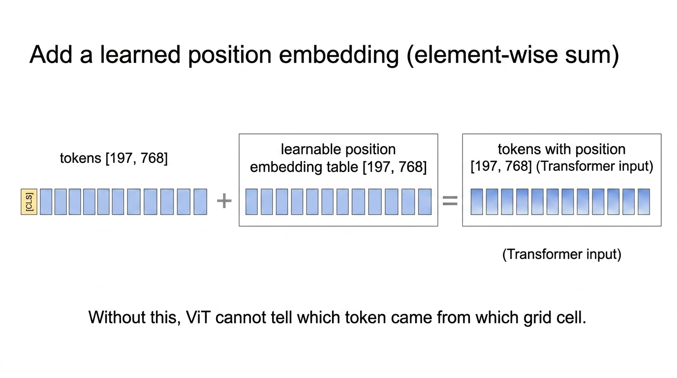
Fig 8. Position embedding is a learnable [1, 197, 768] table added element-wise to the token matrix. Shape is unchanged; only the contents now encode “which grid cell”.

6. The [197, 768] sequence — where shapes finally settle

We now have [B, 197, 768] — 197 tokens, each a 768-dim vector (1 CLS + 196 patches), with position information added. The dimensions to internalise:

• The token count went 196 → 197 — that one extra row is the CLS token.
• The embedding dim stays 768 end to end, both inside every encoder block and through the residual stream. Internal expansions (QKV → 2304, MLP hidden → 3072) all collapse back to 768 before the block ends.

Mental model: CLS changes the token count (196→197), not the vector length (768).

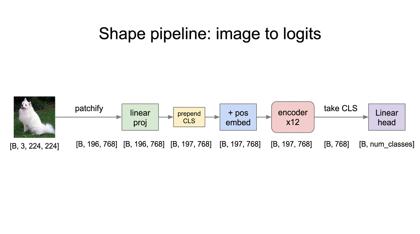
Fig 9. Shape pipeline. Every transition is annotated with its tensor shape. Note how 197 and 768 stay constant from “prepend [CLS]” all the way until “take CLS”.

7. What B is, and what comes OUT of the Transformer

If you worked with CLIP you got used to one number per image: the model returned a single 768-d image embedding. ViT is the same idea, but it is worth being precise about what goes in and what comes out, because two different “768”s show up in this post and they are easy to confuse.

• B is the batch dimension — how many images you process in parallel. Nothing more. Drop it mentally if you want; everything in this post works one image at a time.
• 197 is the token count — 1 CLS + 196 patches. Fixed for ViT-Base/16 at 224×224.
• 768 is the embedding dim D — the length of every token vector.

The Transformer encoder is shape-preserving: feed in [B, 197, 768], get out [B, 197, 768]. Twelve blocks rearrange the contents; they never change the shape.

So how does ViT give you one vector per image, like CLIP? You slice off the CLS row. output[:, 0, :] has shape [B, 768] — that is your image embedding, the direct analog of the CLIP image embedding. For classification you apply one more Linear(768 → num_classes) on top of it.

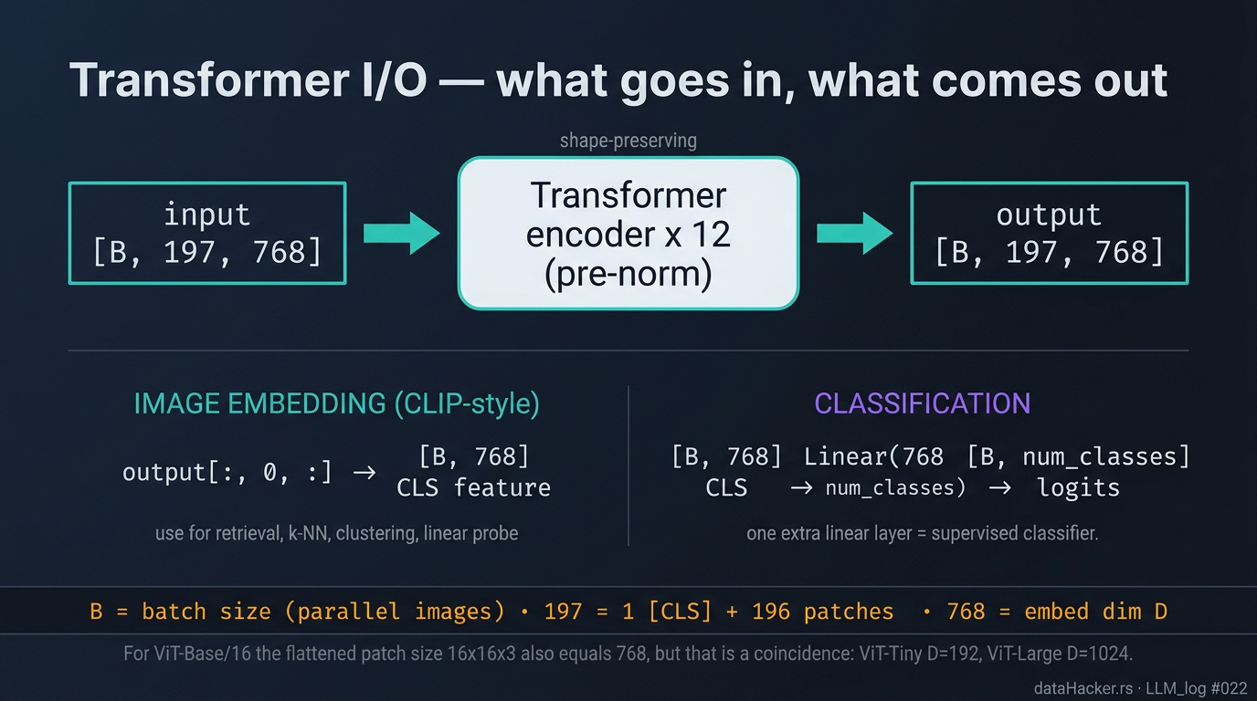
Fig 10. Transformer I/O. Input and output have identical shape [B, 197, 768]. From the output you can either take the CLS row to get a CLIP-style [B, 768] image embedding, or apply one extra linear layer for class scores.

8. The explicit version — same math, no Conv2d

The code in §3 is the compact, production form. Below is the explicit version — no Conv2d, no clever reshapes, explicit loops, one operation per line. Same math, the long way, so you can see exactly what every step does. Batch dimension dropped here for clarity.

import torch
import torch.nn as nn
image_height = 224
image_width  = 224
channels     = 3
patch_size   = 16
embed_dim    = 768
image = torch.randn(channels, image_height, image_width)   # [3, 224, 224]
patches_down   = image_height // patch_size   # 14
patches_across = image_width  // patch_size   # 14
# STEP A: cut the image into 196 squares, one at a time
list_of_patches = []
for row in range(patches_down):          # top to bottom
    for col in range(patches_across):    # left to right
        top    = row * patch_size
        left   = col * patch_size
        bottom = top  + patch_size
        right  = left + patch_size
        one_patch      = image[:, top:bottom, left:right]   # [3, 16, 16]
        one_patch_flat = one_patch.reshape(-1)              # [768]
        list_of_patches.append(one_patch_flat)
patches = torch.stack(list_of_patches)    # [196, 768]
# STEP B: project each raw patch into a learned token
project = nn.Linear(768, embed_dim)       # 768 in -> 768 out
tokens  = project(patches)                # [196, 768]
# STEP C: prepend the CLS token
cls_token = nn.Parameter(torch.zeros(1, embed_dim))   # [1, 768]
sequence  = torch.cat([cls_token, tokens], dim=0)     # [197, 768]
# STEP D: add a learnable position embedding (one row per token)
pos_embed = nn.Parameter(torch.zeros(197, embed_dim)) # [197, 768]
sequence  = sequence + pos_embed                      # [197, 768]
print(sequence.shape)   # torch.Size([197, 768])

In words: chop the image into 196 squares, flatten each to 768 numbers and project them, glue a learnable CLS row on top (197 rows), then add a learnable position row to every token. That 197×768 table is the Transformer’s input.

9. What happens inside the encoder — Q/K/V, multi-head, residual stream

It was always a matrix

One word is a 768-vector. A sentence of 10 words is a [10, 768] matrix — one row per word. ViT’s image is [197, 768] — one row per token. Same object. The Transformer has always eaten a matrix with one row per token; nothing structural changes from text to images.

Q, K, V — the intuition

Each token’s 768-vector is projected three ways:

• Query: “what am I looking for?”
• Key: “what do I offer?”
• Value: “what I hand over if attended to.”

Compare each token’s Query to every Key (dot product) → scores → softmax → take a blended sum of all Values. A token’s new vector is a relevance-weighted mix of every token’s Value. Identical mechanism for words and patches.

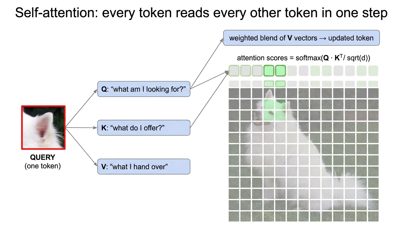
Fig 11. Self-attention. One token’s Query is compared with every Key; the resulting softmax weights blend every Value into the new token vector. With 197 tokens this means a 197 × 197 attention matrix per head.

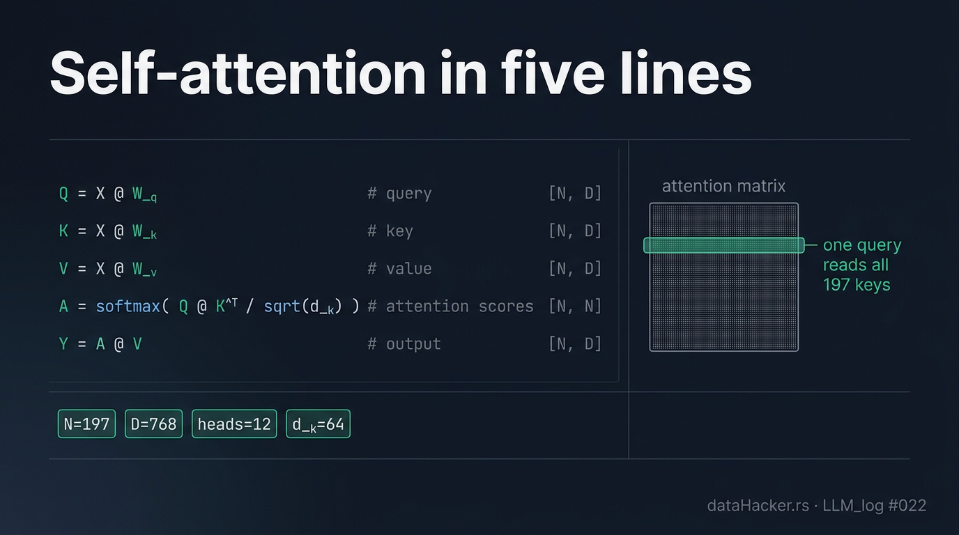
Fig 12. Self-attention in five lines. Three projections to get Q, K, V; one scaled dot-product to get the [N, N] attention matrix; one matmul to blend the values.

Attention, one head, no tricks

import torch
import torch.nn as nn
N, D = 197, 768
X = torch.randn(N, D)          # one image's token matrix (no batch, for clarity)
to_query = nn.Linear(D, D)
to_key   = nn.Linear(D, D)
to_value = nn.Linear(D, D)
Q = to_query(X)   # [197, 768] - what each token is looking for
K = to_key(X)     # [197, 768] - what each token offers
V = to_value(X)   # [197, 768] - what each token will hand over
scores  = Q @ K.T               # [197, 197] every query dotted with every key
scores  = scores / (D ** 0.5)   # scale so the numbers don't blow up
weights = scores.softmax(dim=1) # each row sums to 1: how much to attend to whom
out = weights @ V               # [197, 768] each token = weighted blend of Values
print(out.shape)                # torch.Size([197, 768])

Multi-head, the simple way (a loop over heads)

“Multi-head” just means: split the 768-wide vectors into 12 slices of 64, run the same attention on each slice, and glue the results back together.

H, head_dim = 12, 64    # 12 heads x 64 = 768
def attention(q, k, v):
    s = (q @ k.T) / (q.shape[-1] ** 0.5)
    return s.softmax(dim=1) @ v
outputs = []
for h in range(H):                       # one head at a time
    s = slice(h * head_dim, (h + 1) * head_dim)   # this head's 64 columns
    outputs.append(attention(Q[:, s], K[:, s], V[:, s]))   # [197, 64]
out = torch.cat(outputs, dim=1)          # glue heads back -> [197, 768]
print(out.shape)                         # torch.Size([197, 768])

Different heads can specialise — one tracks edges, another colour, another distant context — and their results concatenate.

How the broken-up image recombines its information

• A patch starts knowing only its own 16×16 pixels.
• Attention is all-to-all: the [197, 197] score matrix lets every patch read from every other patch in a single layer — no locality limit. This is the key break from CNNs.
• The residual stream: each block ADDS to the tokens (x = x + attn(x), x = x + mlp(x)), so information accumulates across the 12 blocks instead of being overwritten.
• The CLS token has no pixels; it attends across all patches every layer and accumulates a whole-image summary that the classifier reads.

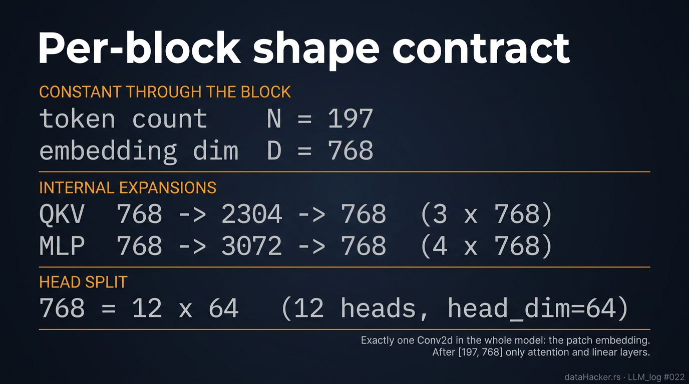
Fig 13. The shape contract every encoder block keeps. 197 and 768 are fixed across the residual stream; QKV and the MLP expand internally and collapse back.

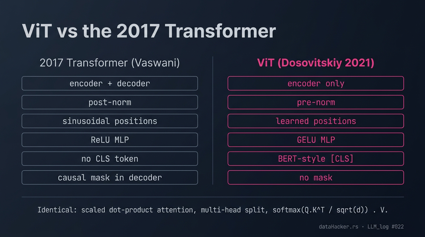
Fig 14. ViT vs the 2017 Transformer. Six engineering differences; the attention primitive itself is unchanged.

10. A minimal Vision Transformer — runnable in one cell

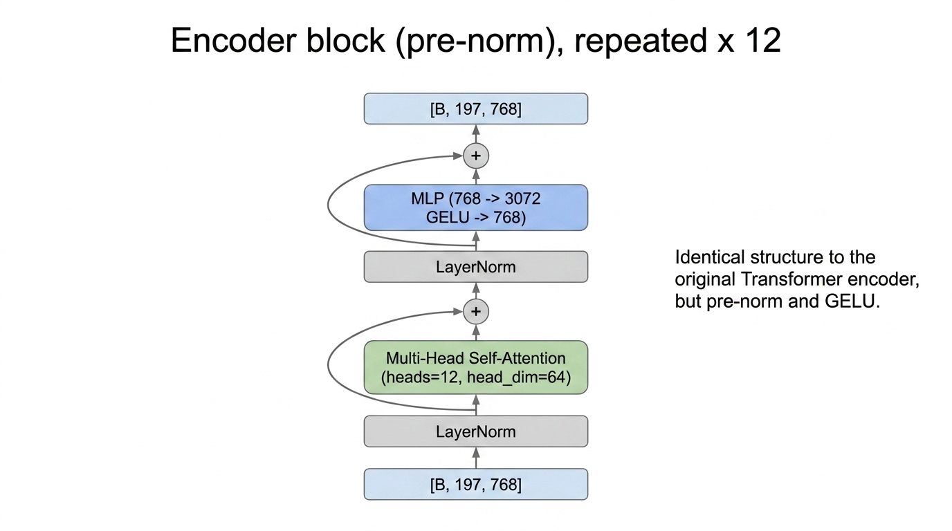
Fig 15. One pre-norm encoder block: LayerNorm → multi-head self-attention → residual → LayerNorm → MLP → residual. Repeated 12 times.

import torch
import torch.nn as nn
class MultiHeadAttention(nn.Module):
    def __init__(self, dim=768, heads=12):
        super().__init__()
        self.heads = heads
        self.head_dim = dim // heads          # 64
        self.qkv = nn.Linear(dim, dim * 3)    # Q, K, V in one layer
        self.proj = nn.Linear(dim, dim)       # output projection
    def forward(self, x):                     # x: [B, N, dim]
        B, N, D = x.shape
        qkv = self.qkv(x).reshape(B, N, 3, self.heads, self.head_dim)
        qkv = qkv.permute(2, 0, 3, 1, 4)      # [3, B, heads, N, head_dim]
        q, k, v = qkv[0], qkv[1], qkv[2]
        scores = (q @ k.transpose(-2, -1)) / self.head_dim ** 0.5
        attn = scores.softmax(dim=-1)
        out = (attn @ v).transpose(1, 2).reshape(B, N, D)   # merge heads
        return self.proj(out)
class MLP(nn.Module):
    def __init__(self, dim=768, hidden=3072):
        super().__init__()
        self.fc1 = nn.Linear(dim, hidden)
        self.act = nn.GELU()
        self.fc2 = nn.Linear(hidden, dim)
    def forward(self, x):
        return self.fc2(self.act(self.fc1(x)))
class Block(nn.Module):                       # pre-norm encoder block
    def __init__(self, dim=768, heads=12):
        super().__init__()
        self.norm1 = nn.LayerNorm(dim)
        self.attn = MultiHeadAttention(dim, heads)
        self.norm2 = nn.LayerNorm(dim)
        self.mlp = MLP(dim, dim * 4)
    def forward(self, x):
        x = x + self.attn(self.norm1(x))      # residual 1
        x = x + self.mlp(self.norm2(x))       # residual 2
        return x
class TinyViT(nn.Module):
    def __init__(self, img=224, p=16, c=3, dim=768, depth=12, heads=12, n_classes=1000):
        super().__init__()
        self.patch = nn.Conv2d(c, dim, kernel_size=p, stride=p)
        n = (img // p) ** 2
        self.cls = nn.Parameter(torch.zeros(1, 1, dim))
        self.pos = nn.Parameter(torch.zeros(1, n + 1, dim))
        self.blocks = nn.ModuleList([Block(dim, heads) for _ in range(depth)])
        self.norm = nn.LayerNorm(dim)
        self.head = nn.Linear(dim, n_classes)
    def forward(self, x):
        x = self.patch(x).flatten(2).transpose(1, 2)           # [B,196,768]
        x = torch.cat([self.cls.expand(x.size(0), -1, -1), x], 1)
        x = x + self.pos                                        # [B,197,768]
        for blk in self.blocks:
            x = blk(x)
        x = self.norm(x)
        return self.head(x[:, 0])                               # CLS -> logits
# quick shape test (random weights):
# m = TinyViT(); print(m(torch.randn(2,3,224,224)).shape)  # [2, 1000]

11. Real pretrained weights — classification + linear probe (no API)

Weights download from the HuggingFace Hub through timm — no API key, no training, no GPU required for inference.

11a. Built-in head — ImageNet classification

# !pip install timm torch pillow
import timm, torch
from PIL import Image
model = timm.create_model('vit_base_patch16_224.augreg2_in21k_ft_in1k',
                          pretrained=True).eval()        # ~86.6M params
cfg = timm.data.resolve_model_data_config(model)
tf  = timm.data.create_transform(**cfg, is_training=False)
img = tf(Image.open('room.jpg').convert('RGB')).unsqueeze(0)   # [1,3,224,224]
with torch.no_grad():
    logits = model(img)                                  # [1, 1000] ImageNet
top5 = logits.softmax(-1).topk(5)
print(top5.indices, top5.values)

11b. Linear probe — classify from the [768] feature vector

Freeze the ViT, pull the 768-dim CLS feature per image, train a tiny classifier on top. No GPU training of the ViT, no API.

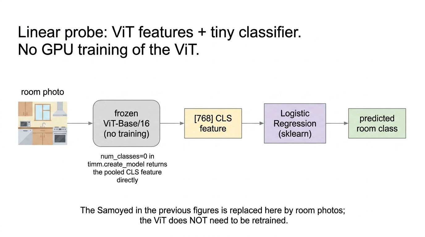
Fig 16. Linear probe. The ViT is frozen and only its 768-d CLS feature is used; a tiny LogisticRegression on top of it does the actual classification. The ViT is not retrained.

# !pip install timm torch scikit-learn pillow
import timm, torch
from PIL import Image
from sklearn.linear_model import LogisticRegression
# num_classes=0  ->  model(x) returns the pooled 768-dim CLS feature directly
extractor = timm.create_model('vit_base_patch16_224', pretrained=True,
                              num_classes=0).eval()
cfg = timm.data.resolve_model_data_config(extractor)
tf  = timm.data.create_transform(**cfg, is_training=False)
@torch.no_grad()
def features(paths):
    xs = torch.stack([tf(Image.open(p).convert('RGB')) for p in paths])
    return extractor(xs).numpy()            # [N, 768] feature vectors

12. What lives in the [768] vector? — circles vs squares, an honest probe

The post has been making a strong claim: the 768-d CLS vector is an “image embedding”. Let’s test it on the simplest possible discrimination — solid white circles vs solid white squares on a black background. The ViT was never trained on synthetic shapes; we just take the pretrained ImageNet model, freeze it, and look at the [768] CLS feature it gives us.

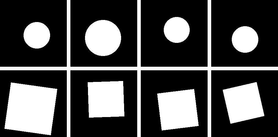
Fig 17. The probe dataset — 50 circles + 50 squares, solid white on black 224×224, random position and size, small rotation jitter for squares. No textures, no colour, nothing the ViT was trained on.

For each of the 100 images we extract the [768] CLS feature with timm.create_model(..., num_classes=0), stack into an X matrix of shape (100, 768), then run PCA down to 2 components and a logistic-regression linear probe on the raw 768 dims.

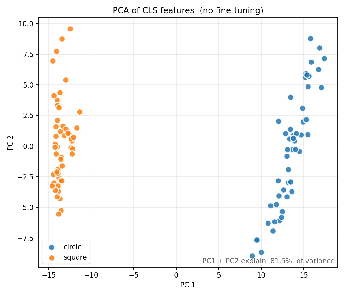
Fig 18. PCA of the 100 CLS features. Two completely disjoint blobs; circles on the right (PC1 ≈ +9 to +18), squares on the left (PC1 ≈ -15 to -11). PC1 alone explains 74.5% of the variance; PC1+PC2 together, 81.5%. A vertical line at PC1 = 0 would separate the classes by hand.

What does the 768-vector actually look like? Average the 50 per-class features and overlay them. The two profiles mostly track each other — both classes are “white shape on black background”, so most dims encode shared structure — but a subset of dims diverges sharply. That subset IS the “circle vs square” signal.

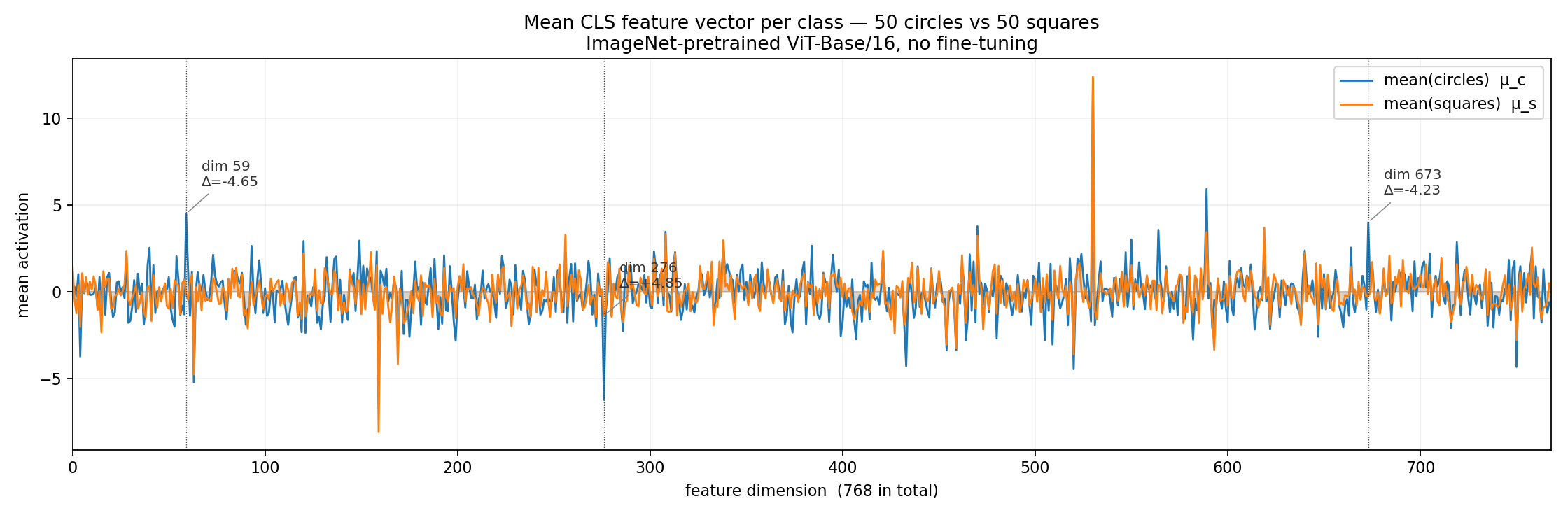
Fig 19. Mean CLS feature per class (blue = circles, orange = squares). The two profiles track each other for most dims (shared “white-on-black” structure), with sharp divergences at certain dimensions — the top three are labelled. 215 out of 768 dimensions have a class-mean difference larger than 1.0; the shape signal is distributed across hundreds of dimensions, not concentrated in one.

13. Summary and what’s next

In Part 1 we built the front end of a Vision Transformer with nothing but a Conv2d, one learnable CLS vector, and one learnable position-embedding table. The Transformer that sits on top is the ordinary encoder we already know.

The dimensions to remember:

• [B, 3, 224, 224] → [B, 196, 768] → [B, 197, 768] → [B, 197, 768] — everything Part 1 does.
• [B, 197, 768] → [B, 197, 768] → [B, 768] → [B, num_classes] — everything Parts 2–3 will do.

Part 2 opens the encoder block (MultiHeadAttention, MLP, pre-norm Block) and validates each module against the real timm ViT-Base/16 weights. Part 3 assembles the full model, loads pretrained weights, runs inference on a real photo, and fine-tunes on Imagenette / Oxford-IIIT Pets / Flowers-102.

References

• Dosovitskiy et al., An Image is Worth 16×16 Words, arXiv:2010.11929 (ICLR 2021).
• Vaswani et al., Attention Is All You Need, arXiv:1706.03762 (NeurIPS 2017).
• Caron et al., Emerging Properties in Self-Supervised ViTs (DINO), arXiv:2104.14294.
• Oquab et al., DINOv2, arXiv:2304.07193.
• timm ViT weights: vit_base_patch16_224.augreg2_in21k_ft_in1k on the HF Hub.
• timm feature extraction: huggingface.co/docs/timm/en/feature_extraction.
• DINOv2: github.com/facebookresearch/dinov2.

dataHacker.rs — LLM_log #022 — Vision Transformer From Scratch, Part 1 — Vladimir Matic. Diagrams generated with Gemini 3 Pro Image Preview.