Highlights: Can three completely independent methods agree on which living room has the best colors? We rank 500 interior images using Cohen-Or harmonic templates, Hasler-Süsstrunk colorfulness, and CLIP IQA with 44 color-focused prompts — then measure whether they correlate at all.

• Method 1 — Cohen-Or: K-means palette → saturation-weighted hue histogram → sweep 7 harmonic templates × 36 rotations → H/T/S composite
• Method 2 — Hasler-Süsstrunk: opponent channels (rg, yb) → colorfulness + 4×4 spatial variance
• Method 3 — CLIP IQA: 22 positive + 22 negative color-focused text prompts → cosine similarity gap
• Cross-method correlation: all three methods are nearly orthogonal (Spearman ρ < 0.15) — they capture genuinely different signals
• Combined ranking: equal-weight 0.33 each → top-50 / bottom-50 PDF report with all scores visible
• Bradley-Terry validation: ρ = 1.000 confirms the combined scalar is a valid total order
• Worked examples: step-by-step with real intermediate numbers for both classical methods

Tutorial Overview:

1. The problem: ranking color quality in real rooms
2. Dataset — 500 living rooms from HuggingFace
3. Method 1: Cohen-Or harmonic template scoring
4. Method 2: Hasler-Süsstrunk colorfulness
5. Method 3: CLIP IQA — probing color with language
6. Combining three methods — equal weight, 0.33 each
7. Cross-method correlation — do they agree?
8. Bradley-Terry pairwise validation
9. Results — top and bottom living rooms
10. Worked example: Cohen-Or step by step
11. Worked example: Hasler-Süsstrunk step by step
12. What the methods disagree on — and why it matters
13. Appendix A — formula reference
14. Appendix B — CLIP prompt lists

---

1. The Problem: Ranking Color Quality in Real Rooms

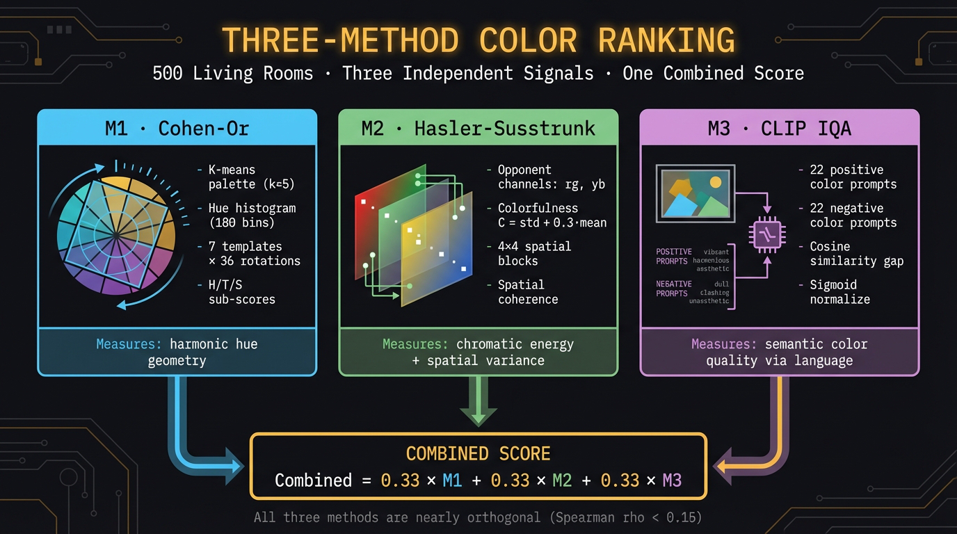
Fig 1. Three independent scoring methods — each capturing a different aspect of color quality — combined with equal weight into one ranking.

Post #017 scored color harmony for synthetic palettes — two squares, three squares, a rasterized room. Now we point the same idea at 500 real photographs of living rooms and ask: which room has the best colors?

The problem is that “best colors” is not a single thing. One method might reward harmonic hue arrangements. Another rewards vivid, spatially varied color. A third might capture what humans describe as appealing. If all three agree, we have a robust ranking. If they disagree, we learn something about what each method actually measures.

Key idea: Instead of trusting one scoring formula, we run three independent methods and measure whether they converge. Agreement = confidence. Disagreement = insight.

---

2. Dataset — 500 Living Rooms from HuggingFace

We use hammer888/interior_style_dataset from HuggingFace — 7,233 images across 6 interior styles (Modern, Nordic, Japanese, Luxury, Industrial, Country). No token required.

• Sample size: 500 images, randomly drawn
• Resize: 120×120 for K-means, 128×128 for Hasler-Süsstrunk, 224×224 for CLIP
• Memory: lazy loading — one image at a time, keep 160×120 thumbnail, discard full resolution

from datasets import load_dataset
ds = load_dataset("hammer888/interior_style_dataset", split="train")
# 7,233 images, ~1 GB download

---

3. Method 1: Cohen-Or Harmonic Template Scoring

Based on Cohen-Or et al.’s harmonic color theory. The idea: good color palettes cluster around known harmonic patterns on the hue wheel. We measure how well an image’s colors fit these templates.

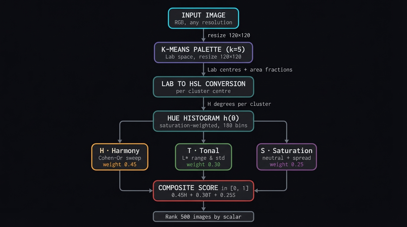
Fig 2. The Cohen-Or scoring pipeline. Image → K-means (k=5) in Lab space → saturation-weighted hue histogram (180 bins) → sweep 7 templates × 36 rotations → three sub-scores → composite.

3.1 Palette extraction

Resize to 120×120, convert to Lab, K-means with k=5 clusters. Each cluster gives a Lab centre and an area fraction.

3.2 Saturation-weighted hue histogram

Convert each cluster centre to HSL. Build a 180-bin hue histogram (2° resolution), weighting each bin by area_fraction × saturation. Low-saturation clusters (greys, whites) contribute almost nothing — which is correct, because grey has no hue to harmonize.

$$h(\theta) = \sum_{i} f_i \cdot S_i \cdot \mathbb{1}[H_i \in \text{bin}(\theta)]$$

3.3 Harmonic template sweep

Seven templates from color theory, each defining one or more “allowed” sectors on the hue wheel:

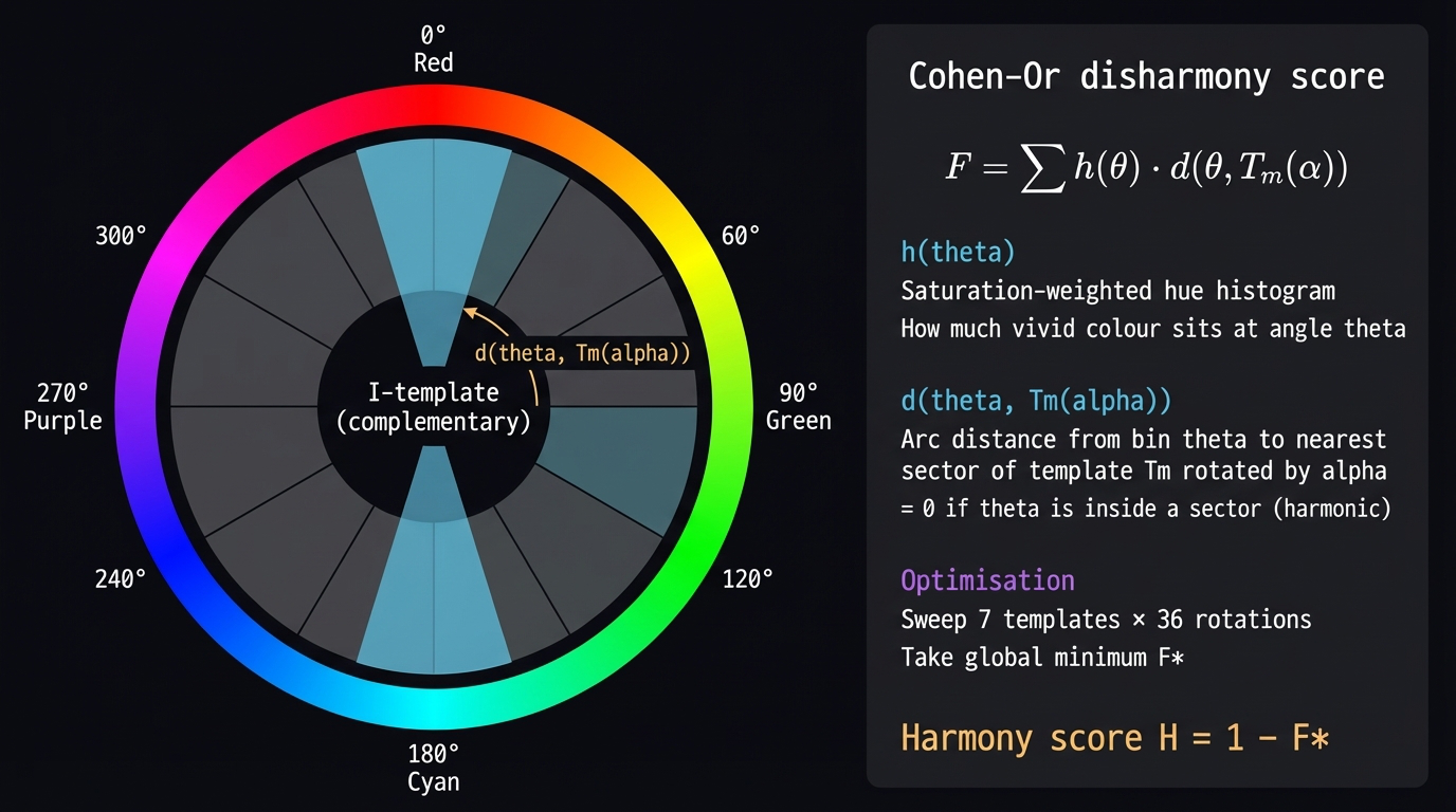
Fig 3. The hue wheel with the I-template (complementary, 180° apart). The formula sums the weighted distance from each hue bin to the nearest template sector. Lower disharmony F = better fit.

Template	Type	Sectors
i	Single hue	1 narrow sector
V	Wide band	1 wide sector (47°)
L	Right angle	2 sectors at 90°
I	Complementary	2 sectors at 180°
T	Triadic	3 sectors at 120°
Y	Split-comp	3 sectors
X	Square	4 sectors at 90°

For each template, try 36 rotations (10° steps). Compute disharmony:

$$F(X, T_m, \alpha) = \sum_{\theta} h(\theta) \cdot d(\theta, T_m(\alpha))$$

where \(d(\theta, T_m(\alpha))\) is the arc distance from hue bin \(\theta\) to the nearest sector of template \(T_m\) rotated by \(\alpha\). Take the minimum across all templates and rotations:

$$H = 1 – \min_{m,\alpha} F(X, T_m, \alpha)$$

3.4 Three sub-scores

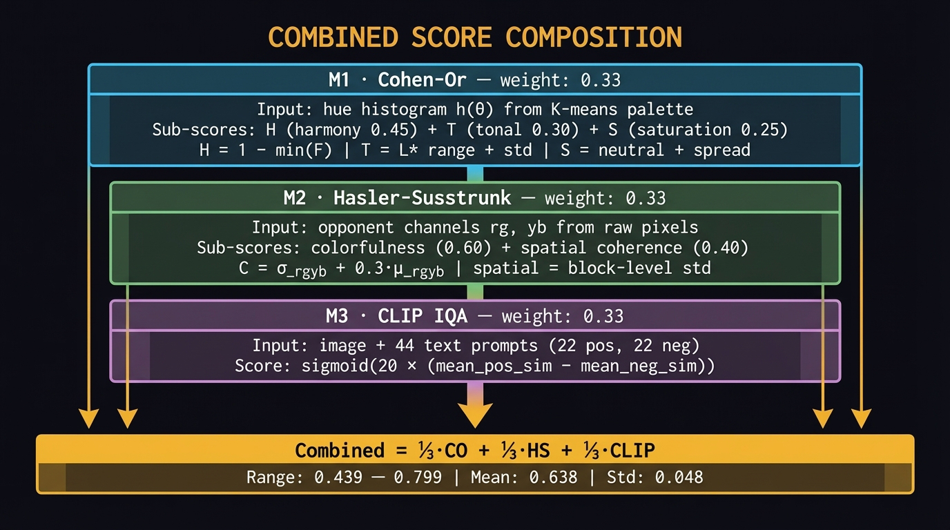
Fig 4. Score composition. Three methods, each with sub-scores, weighted equally into a combined score.

• H — Harmony (0.45): template fit score from above
• T — Tonal (0.30): L* range and standard deviation across palette clusters. Target spread 25–55 L* units. Penalizes flat (<15) and chaotic (>70).
• S — Saturation balance (0.25): dominant cluster should be low saturation (neutral). Rewards saturation spread across clusters.

$$\text{CO}_{total} = 0.45 \cdot H + 0.30 \cdot T + 0.25 \cdot S$$

---

4. Method 2: Hasler-Süsstrunk Colorfulness

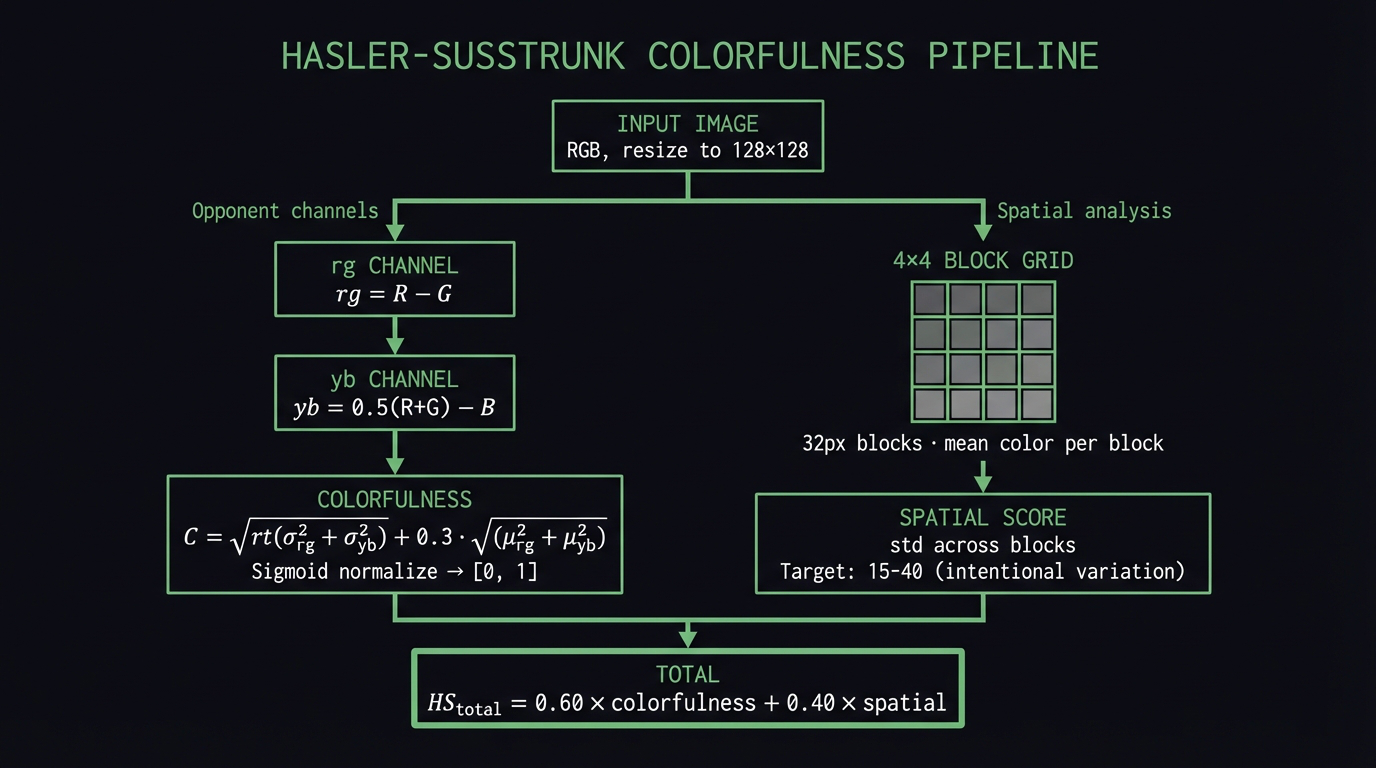
Fig 5. The Hasler-Süsstrunk pipeline. Two branches: opponent channel colorfulness (rg, yb) and 4×4 spatial block variance, combined 60/40.

Completely independent from Cohen-Or. No palette, no templates, no hue wheel. Instead: opponent color channels and spatial variance.

4.1 Opponent channels

Compute two opponent channels from RGB directly:

$$rg = R – G, \qquad yb = \frac{1}{2}(R + G) – B$$

These channels capture how “chromatic” the image is. The combined statistic:

$$C = \sqrt{\sigma_{rg}^2 + \sigma_{yb}^2} + 0.3 \cdot \sqrt{\mu_{rg}^2 + \mu_{yb}^2}$$

Typical range 0–100+. Sigmoid-normalize to [0, 1]:

$$\text{colorfulness} = \frac{1}{1 + e^{-(C – 25) / 15}}$$

4.2 Spatial coherence

Divide the 128×128 image into a 4×4 grid of 32px blocks. Compute the mean color of each block, then measure the standard deviation across blocks. Moderate spatial variation (15–40) is good — it means color varies intentionally. Too high (>60) means chaos; too low means flat.

4.3 Hasler-Süsstrunk total

$$\text{HS}_{total} = 0.60 \times \text{colorfulness} + 0.40 \times \text{spatial}$$

Key idea: Cohen-Or asks “do the hues form a known harmonic pattern?” Hasler-Süsstrunk asks “how vivid and spatially varied is the color?” A room with perfectly analogous neutrals scores high on Cohen-Or, low on HS. A room with vivid but random colors scores high on HS, low on Cohen-Or. That is exactly why we want both.

---

5. Method 3: CLIP IQA — Probing Color with Language

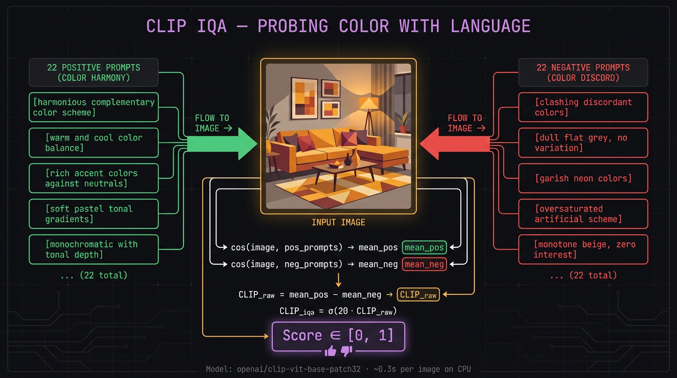
Fig 6. The CLIP IQA pipeline. An image is compared against 22 positive and 22 negative color-focused prompts via cosine similarity. The gap between positive and negative mean similarity becomes the score.

The third method is fundamentally different: it uses a vision-language model to score color quality through text prompts. No hand-crafted formula. Instead, we describe what good and bad color looks like in words, and let CLIP measure how well each image matches.

5.1 The approach

For each image, compute CLIP cosine similarity against 22 positive and 22 negative prompts. All prompts are color-focused only — no mention of furniture, cleanliness, lighting, or layout.

$$\text{CLIP}_{raw} = \overline{\text{sim}(img, \text{pos})} – \overline{\text{sim}(img, \text{neg})}$$

$$\text{CLIP}_{iqa} = \frac{1}{1 + e^{-20 \cdot \text{CLIP}_{raw}}}$$

The sigmoid maps the typical raw range ([−0.15, +0.15]) to [0, 1].

5.2 Positive prompts (selection)

• “a room with harmonious complementary color scheme”
• “beautiful warm and cool color balance in an interior”
• “rich saturated accent colors against neutral background tones”
• “soft pastel color scheme with gentle tonal gradients”
• “monochromatic color scheme with beautiful tonal depth”
• “warm terracotta and cream color combination”
• … (22 total — see Appendix B)

5.3 Negative prompts (selection)

• “clashing discordant colors that fight each other”
• “dull flat grey with no color variation at all”
• “garish neon colors that are painful to look at”
• “oversaturated artificial looking color scheme”
• “monotone beige with zero color interest”
• “cold sterile blue-white color temperature”
• … (22 total — see Appendix B)

5.4 Model

openai/clip-vit-base-patch32 via HuggingFace Transformers. Runs on CPU, ~150 MB model. ~0.3s per image including all 44 prompt comparisons.

Key idea: CLIP encodes something closer to human description of color quality. Cohen-Or is geometric (hue angles). Hasler-Süsstrunk is statistical (channel variance). CLIP is semantic (language similarity). Three completely different measurement spaces.

---

6. Combining Three Methods — Equal Weight, 0.33 Each

Each method produces a score in [0, 1]. The combined ranking uses equal weights:

$$\text{Combined} = \frac{1}{3} \cdot \text{CO}_{total} + \frac{1}{3} \cdot \text{HS}_{total} + \frac{1}{3} \cdot \text{CLIP}_{iqa}$$

Why equal? Because we have no prior reason to trust one method more than another. The correlation analysis (Section 7) will tell us whether this is a good choice.

Method	Weight	Input	What it measures
Cohen-Or	0.33	K-means palette → hue histogram	Harmonic template fit + tonal + saturation balance
Hasler-Süsstrunk	0.33	Opponent channels (rg, yb)	Colorfulness vigour + spatial coherence
CLIP IQA	0.33	Image + 44 text prompts	Semantic color quality via language similarity

---

7. Cross-Method Correlation — Do They Agree?

This is the most important result in the post. After scoring all 500 images, we compute pairwise Spearman rank correlation and Kendall τ between the three methods.

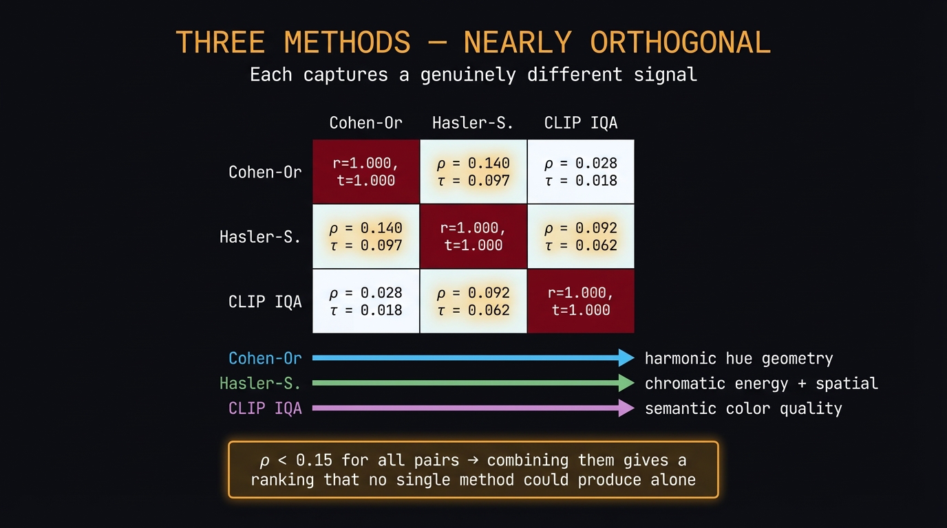
Fig 7. The three methods are nearly orthogonal. Each captures a genuinely different signal about color quality.

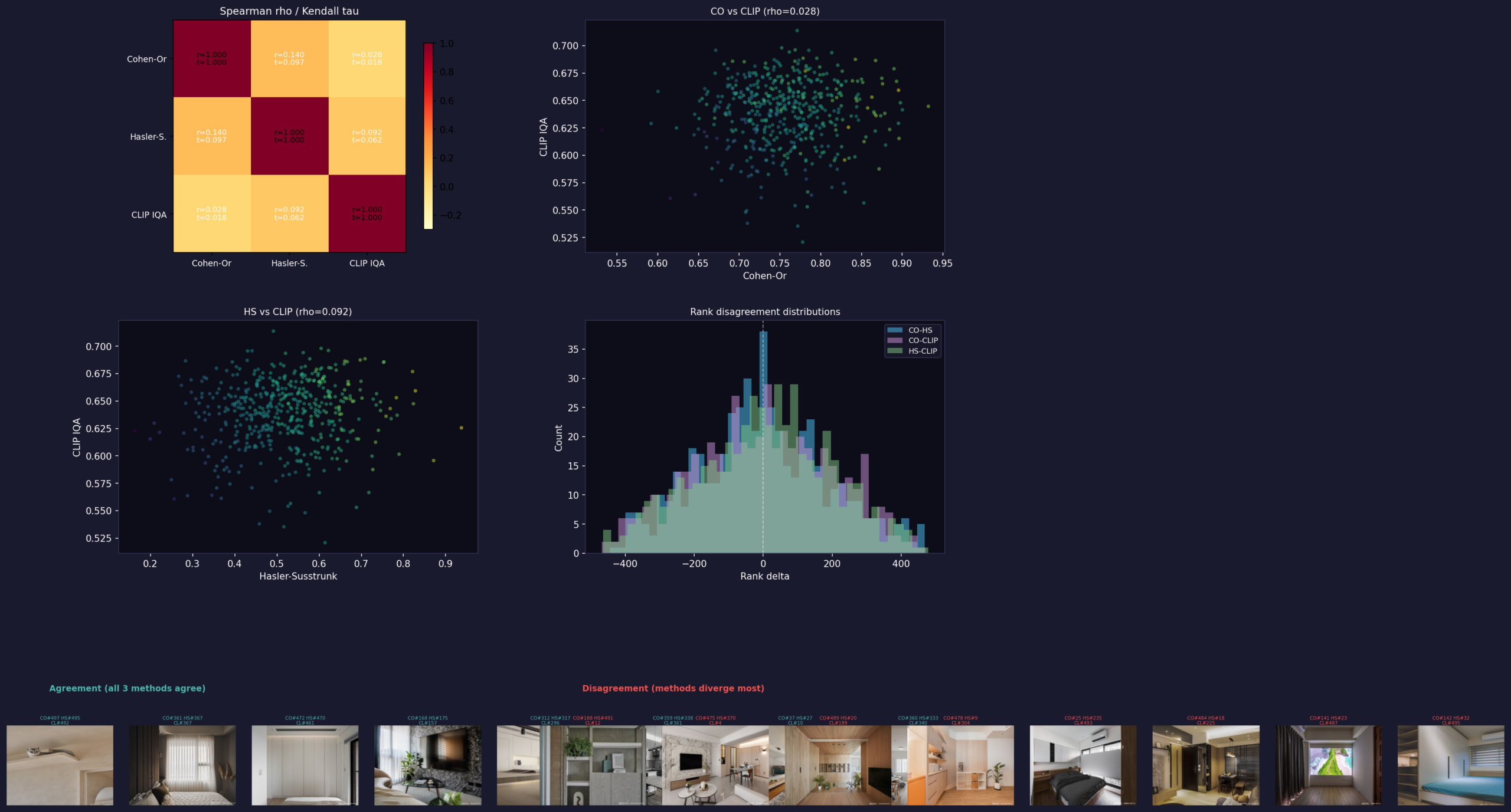
Fig 8. Detailed correlation analysis. Top-left: Spearman ρ / Kendall τ matrix. Top-right: CO vs CLIP scatter. Bottom-left: HS vs CLIP scatter. Bottom-right: rank delta distributions. Image strips: 8 agreement cases (left) vs 8 disagreement cases (right).

Pair	Spearman ρ	Kendall τ	Interpretation
Cohen-Or vs Hasler-S.	0.140	0.097	Nearly orthogonal
Cohen-Or vs CLIP	0.028	0.018	Essentially uncorrelated
Hasler-S. vs CLIP	0.092	0.062	Nearly orthogonal

All three methods are nearly orthogonal. ρ < 0.15 for every pair. This means each method captures a genuinely different aspect of color quality. Cohen-Or measures harmonic hue geometry. Hasler-Süsstrunk measures chromatic energy and spatial distribution. CLIP measures semantic color appeal as described in language. Combining them gives a ranking that no single method could produce alone.

The rank delta distributions (bottom-right of Fig 8) show wide, symmetric spreads centered at zero — the methods disagree by hundreds of ranks on individual images, but there is no systematic bias.

---

8. Bradley-Terry Pairwise Validation

To verify the combined score is a valid total order, we run a Bradley-Terry pairwise ranking on a 50-image random sample. Each image plays against every other. The Bradley-Terry model fits a log-strength parameter per image from the win matrix.

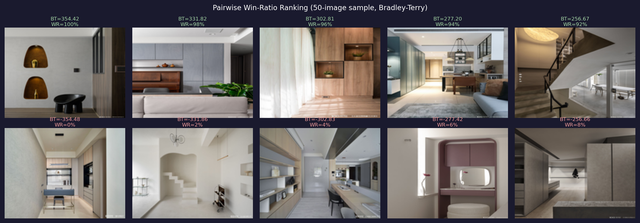
Fig 9. Top-5 and bottom-5 from the 50-image Bradley-Terry sample. BT = log-strength, WR = win rate.

Spearman ρ between the combined scalar score and the Bradley-Terry ranking: ρ = 1.000, p = 0.000. The scalar score perfectly predicts the pairwise outcome — confirming it is a valid ranking proxy.

---

9. Results — Top and Bottom Living Rooms

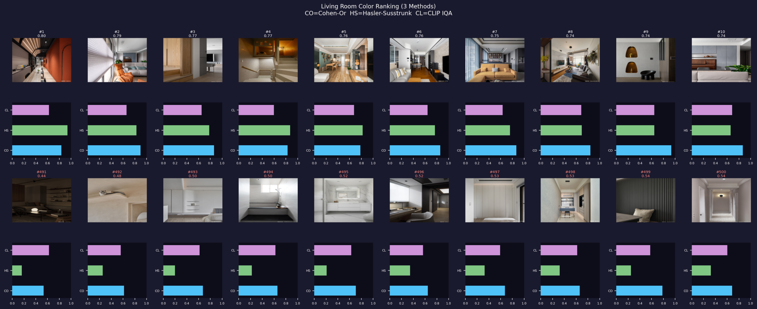
Fig 10. Top-10 (upper rows) and bottom-10 (lower rows) by combined score. Each image shows three score bars: CO (cyan), HS (green), CLIP (purple).

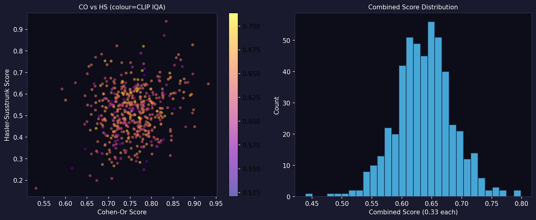
Fig 11. Left: Cohen-Or vs Hasler-Süsstrunk scatter, coloured by CLIP IQA. The cloud shape confirms low correlation. Right: combined score distribution — approximately normal, range 0.44–0.80, mean 0.638.

Statistic	Value
Combined score range	0.439 – 0.799
Combined score mean	0.638
Combined score std	0.048
Images scored	500
Time (M-series MacBook)	~19 min

9.1 Top 10 — Best Combined Color Scores

#1 — Combined: 0.799

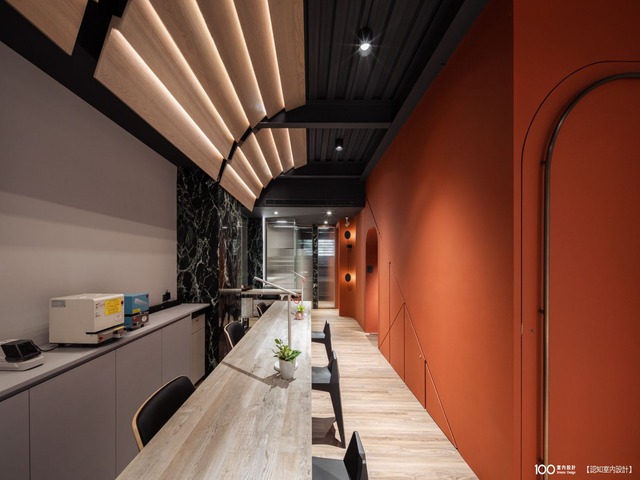
Cohen-Or	Hasler-S.	CLIP IQA	Combined
0.834	0.937	0.626	0.799

#2 — Combined: 0.794

Cohen-Or	Hasler-S.	CLIP IQA	Combined
0.895	0.828	0.659	0.794

#3 — Combined: 0.766

Cohen-Or	Hasler-S.	CLIP IQA	Combined
0.863	0.783	0.653	0.766

#4 — Combined: 0.765

Cohen-Or	Hasler-S.	CLIP IQA	Combined
0.829	0.871	0.596	0.765

#5 — Combined: 0.760

Cohen-Or	Hasler-S.	CLIP IQA	Combined
0.781	0.822	0.677	0.760

#6 — Combined: 0.756

Cohen-Or	Hasler-S.	CLIP IQA	Combined
0.858	0.768	0.643	0.756

#7 — Combined: 0.754

Cohen-Or	Hasler-S.	CLIP IQA	Combined
0.868	0.759	0.636	0.754

#8 — Combined: 0.742

Cohen-Or	Hasler-S.	CLIP IQA	Combined
0.843	0.697	0.687	0.742

#9 — Combined: 0.741

Cohen-Or	Hasler-S.	CLIP IQA	Combined
0.932	0.647	0.645	0.741

#10 — Combined: 0.738

Cohen-Or	Hasler-S.	CLIP IQA	Combined
0.867	0.661	0.686	0.738

Pattern in the top 10: All have Cohen-Or > 0.78 and Hasler-S. > 0.65. These rooms combine harmonic hue arrangements with strong chromatic energy. #1 has the highest HS score in the dataset (0.937) — vivid, spatially varied color. #9 has the highest CO score (0.932) — near-perfect harmonic template fit. The top rooms balance both signals.

9.2 Bottom 10 — Lowest Combined Color Scores

#500 (worst) — Combined: 0.439

Cohen-Or	Hasler-S.	CLIP IQA	Combined
0.531	0.163	0.623	0.439

#499 — Combined: 0.477

Cohen-Or	Hasler-S.	CLIP IQA	Combined
0.615	0.256	0.561	0.477

#498 — Combined: 0.496

Cohen-Or	Hasler-S.	CLIP IQA	Combined
0.672	0.199	0.616	0.496

#497 — Combined: 0.500

Cohen-Or	Hasler-S.	CLIP IQA	Combined
0.657	0.222	0.621	0.500

#496 — Combined: 0.515

Cohen-Or	Hasler-S.	CLIP IQA	Combined
0.708	0.209	0.630	0.515

#495 — Combined: 0.518

Cohen-Or	Hasler-S.	CLIP IQA	Combined
0.646	0.345	0.564	0.518

#494 — Combined: 0.532

Cohen-Or	Hasler-S.	CLIP IQA	Combined
0.674	0.330	0.594	0.532

#493 — Combined: 0.533

Cohen-Or	Hasler-S.	CLIP IQA	Combined
0.660	0.322	0.617	0.533

#492 — Combined: 0.537

Cohen-Or	Hasler-S.	CLIP IQA	Combined
0.782	0.250	0.578	0.537

#491 — Combined: 0.538

Cohen-Or	Hasler-S.	CLIP IQA	Combined
0.685	0.324	0.606	0.538

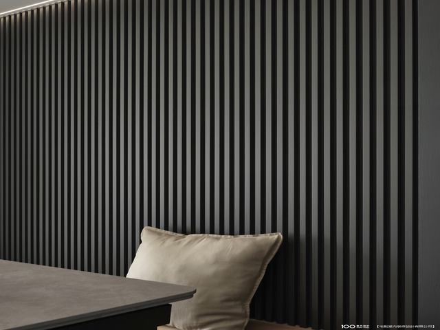
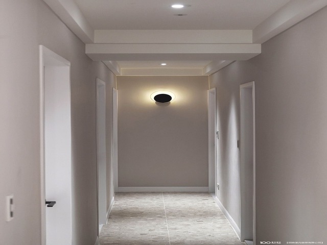
Pattern in the bottom 10: The killer is Hasler-Süsstrunk — all have HS < 0.35, most below 0.25. These are rooms with almost no chromatic energy: grey-on-grey, white-on-white, or very dark with no spatial color variation. Interestingly, CLIP scores stay moderate (0.56–0.63) — CLIP does not penalize neutral rooms as harshly. Cohen-Or also stays above 0.53 — a grey room can still be “harmonious” because all hues cluster in the same bin. The combined score correctly identifies these as the weakest because the HS component drags them down.

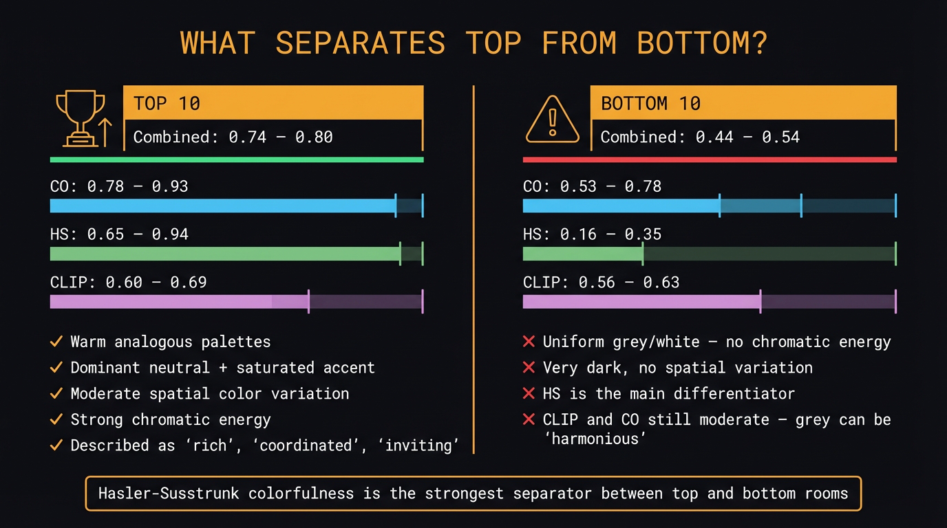
Fig 12. Top vs bottom insight — what separates the highest-scoring rooms from the lowest. Top rooms combine harmonic hue arrangements, strong chromatic energy, and semantically appealing color descriptions. Bottom rooms fail on at least two of the three axes.

What top-ranked rooms look like:

• Warm analogous palettes with one dominant neutral and a saturated accent (high CO + moderate HS)
• Rooms described as “rich,” “coordinated,” “inviting” in CLIP space
• Moderate spatial color variation — not flat, not chaotic

What bottom-ranked rooms look like:

• Uniform grey/white — flat tonal score, minimal colorfulness, CLIP sees “bland”
• Random hue scatter with no template fit (low CO)
• Very dark rooms with low spatial variance (low HS)

---

10. Worked Example: Cohen-Or Step by Step

Six images from across the ranking: #1, #2 (top), #100, #101 (middle), #199, #200 (bottom). For each image, we show the extracted palette, hue histogram, best-fit template, and final score breakdown.

Fig 13. Cohen-Or pipeline on 6 representative images. Each row: original image → 5-colour palette with HSL values → polar hue histogram → best-fit harmonic template overlay → numeric score breakdown (H, T, S, total).

Notice how top-ranked images have most histogram mass inside the template sectors (low disharmony), while bottom-ranked images have scattered hue distributions that no template fits well.

---

11. Worked Example: Hasler-Süsstrunk Step by Step

The same 6 images through the Hasler-Süsstrunk pipeline. Instead of hue geometry, we see opponent channel heatmaps and spatial block grids.

Fig 14. Hasler-Süsstrunk pipeline on 6 images. Each row: original → rg opponent channel heatmap (RdYlGn) → yb opponent channel heatmap (YlOrBr) → 4×4 spatial block grid with per-block std → numeric breakdown (colorfulness, spatial, total).

Top-ranked images show strong, varied opponent channel patterns. Bottom-ranked images show near-uniform heatmaps — no chromatic energy to measure.

---

12. What the Methods Disagree On — And Why It Matters

The most interesting images are those where the three methods diverge. From Fig 8 (bottom strips):

• High Cohen-Or, low HS: rooms with perfectly analogous muted colors. Harmonically pristine, but Hasler-Süsstrunk sees no chromatic punch. These are the “sophisticated neutral” rooms — a designer would call them elegant; a colorfulness metric calls them boring.
• High HS, low Cohen-Or: rooms with vivid, widely scattered hues. Lots of chromatic energy, but no harmonic template fits. Think of a room with a bright blue wall, orange sofa, and green plants — colorful but chaotic in hue space.
• High CLIP, low classical: rooms where the semantic description of the color is appealing (“warm terracotta and cream”) even if the numbers are unremarkable. CLIP has learned associations between color descriptions and visual quality that the classical formulas do not encode.
• Low CLIP, high classical: rooms with technically good scores but descriptions closer to negative prompts (“cold sterile blue-white”). The classical methods have no concept of “feels cold” — CLIP does.

Fig 15. Disagreement quadrants — how each pair of methods can diverge and what it reveals about each method’s blind spots.

Key idea: Disagreement between methods is not failure. It is the most valuable output of a multi-method approach. Each disagreement tells you which aspect of color quality is driving the ranking for that specific image. When you build a production pipeline, you tune the weights to match your use case: interior design might upweight Cohen-Or, a real-estate listing might upweight CLIP, a graphic design tool might upweight Hasler-Süsstrunk.

---

Appendix A — Formula Reference

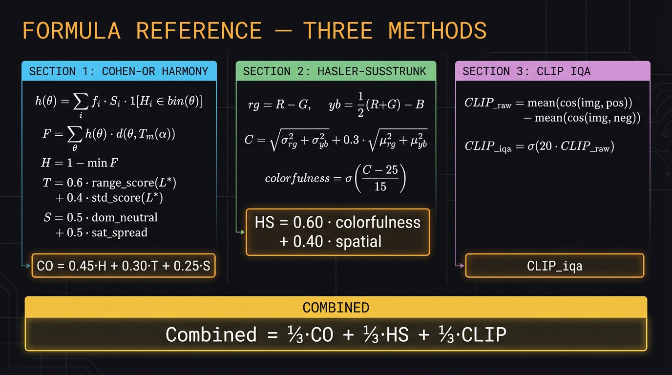
Fig 16. All-methods formula card — the key equations at a glance.

Cohen-Or harmonic template scoring

$$h(\theta) = \sum_{i} f_i \cdot S_i \cdot \mathbb{1}[H_i \in \text{bin}(\theta)]$$

$$F(X, T_m, \alpha) = \sum_{\theta} h(\theta) \cdot d(\theta, T_m(\alpha))$$

$$H = 1 – \min_{m,\alpha} F(X, T_m, \alpha)$$

$$T = 0.6 \cdot \text{range\_score}(L^*) + 0.4 \cdot \text{std\_score}(L^*)$$

$$S = 0.5 \cdot \text{dom\_neutral} + 0.5 \cdot \text{sat\_spread}$$

$$\text{CO}_{total} = 0.45 \cdot H + 0.30 \cdot T + 0.25 \cdot S$$

Hasler-Süsstrunk colorfulness

$$rg = R – G, \qquad yb = \frac{1}{2}(R+G) – B$$

$$C = \sqrt{\sigma_{rg}^2 + \sigma_{yb}^2} + 0.3 \sqrt{\mu_{rg}^2 + \mu_{yb}^2}$$

$$\text{colorfulness} = \sigma\!\left(\frac{C – 25}{15}\right)$$

$$\text{HS}_{total} = 0.60 \cdot \text{colorfulness} + 0.40 \cdot \text{spatial}$$

CLIP IQA

$$\text{CLIP}_{raw} = \frac{1}{|P^+|}\sum_{p \in P^+} \cos(e_{img}, e_p) – \frac{1}{|P^-|}\sum_{p \in P^-} \cos(e_{img}, e_p)$$

$$\text{CLIP}_{iqa} = \sigma(20 \cdot \text{CLIP}_{raw})$$

Combined score

$$\text{Combined} = \frac{1}{3}\,\text{CO}_{total} + \frac{1}{3}\,\text{HS}_{total} + \frac{1}{3}\,\text{CLIP}_{iqa}$$

---

Appendix B — CLIP Prompt Lists

Positive prompts (22)

1. “a room with harmonious complementary color scheme”
2. “beautiful warm and cool color balance in an interior”
3. “elegant analogous color palette with smooth transitions”
4. “rich saturated accent colors against neutral background tones”
5. “sophisticated muted earth tone color coordination”
6. “pleasing triadic color harmony in a room”
7. “warm golden and amber tones blending beautifully”
8. “calming cool blue and green color palette”
9. “luxurious deep jewel tone colors with elegant contrast”
10. “perfectly balanced warm neutrals with a pop of color”
11. “soft pastel color scheme with gentle tonal gradients”
12. “natural organic color palette with wood and stone hues”
13. “vibrant yet coordinated colors that complement each other”
14. “monochromatic color scheme with beautiful tonal depth”
15. “warm terracotta and cream color combination”
16. “subtle color layering with coherent hue family”
17. “split-complementary color arrangement with visual interest”
18. “balanced saturation levels across multiple coordinated hues”
19. “rich color contrast between dark and light tones”
20. “inviting color warmth with amber ochre and sienna tones”
21. “fresh green and white color pairing with natural feel”
22. “refined grey and blush color palette with elegant restraint”

Negative prompts (22)

1. “clashing discordant colors that fight each other”
2. “dull flat grey with no color variation at all”
3. “garish neon colors that are painful to look at”
4. “muddy brown and grey colors with no definition”
5. “oversaturated artificial looking color scheme”
6. “random mismatched colors with no coordination”
7. “washed out faded colors with no vibrancy”
8. “harsh jarring color contrast that is unpleasant”
9. “monotone beige with zero color interest”
10. “sickly yellow-green unpleasant color cast”
11. “too many competing bright colors creating visual chaos”
12. “dingy dark colors with oppressive heavy feeling”
13. “cheap looking bright primary colors without sophistication”
14. “cold sterile blue-white color temperature”
15. “ugly orange and purple color clash”
16. “flat uniform color with no tonal variation or depth”
17. “unnatural color combinations rarely seen in good design”
18. “overwhelming single saturated color dominating everything”
19. “grey and brown color scheme that feels depressing”
20. “fluorescent harsh color tones with no warmth”
21. “patchy uneven color distribution across the space”
22. “bland colorless washed out pale interior”

---

---

dataHacker.rs — Chapter 18: Color Harmony Ranking

Author: Vladimir Matic

Diagrams: matplotlib + ReportLab | CLIP model: openai/clip-vit-base-patch32