LLM_log #013: Latent Space — From AutoEncoders to the Engine Inside Stable Diffusion
Highlights:
Every time you use Stable Diffusion, DALL-E, or Sora, the model never touches a single pixel during its main computation. It works entirely inside a compressed, structured space of floating-point numbers — a latent space learned by a VAE. In this post we build that space from scratch. We start from the simplest possible compression — an AutoEncoder on MNIST digits — understand why it fails at generation, fix it with the VAE’s probabilistic trick, then scale to real human faces. By the end, the geometry makes intuitive sense. So let’s begin!
Tutorial Overview:
- Why Compress at All?
- AutoEncoder: The Bottleneck Idea
- Visualising the Latent Space
- Why AutoEncoders Are Bad Generators
- VAE: Adding a Distribution to the Bottleneck
- The Loss Function: A Tug-of-War
- Comparing the Two Latent Spaces
- Scaling Up: Face VAE on CelebA
- Random Sampling and Interpolation
- Are VAEs Dead? Where They Live Today
- Summary
1. Why Compress at All?
A 28×28 grayscale image is a vector of 784 numbers. That sounds manageable. But consider a 512×512 RGB image — that’s 786,432 numbers. Training a diffusion model directly on that space is computationally brutal.
More importantly: most of those 784 (or 786,432) numbers are not independent. Natural images are highly structured. The pixel at position (14, 14) is almost certainly similar to the pixel at (14, 15). The information content is far lower than the dimensionality suggests. The manifold hypothesis formalises this intuition: natural data lies on a low-dimensional manifold embedded in a very high-dimensional space.
Traditional compression (ZIP, JPEG) finds that manifold using hand-crafted rules — DCT coefficients, Huffman coding. The ML approach is different: let the data teach the model what matters. The result is not a compression algorithm. It is a learned coordinate system.
Key idea: The goal is not to store data more efficiently. It is to find a space where the data’s underlying structure is explicit and navigable — where you can interpolate between a “3” and a “7” and get something meaningful in between.
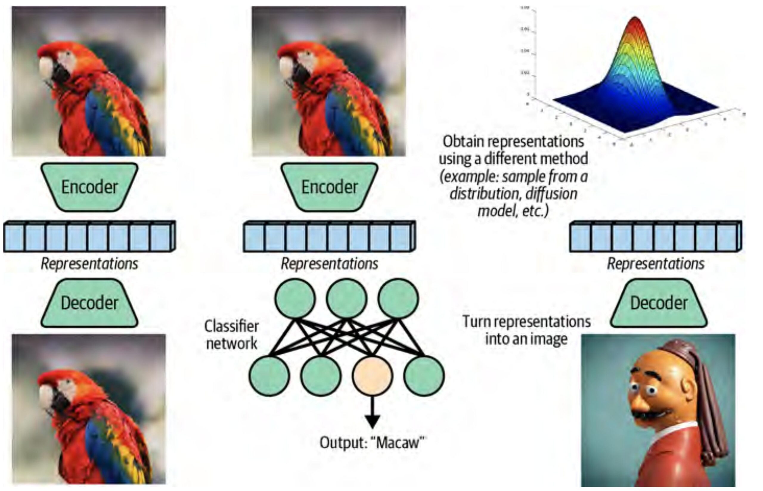
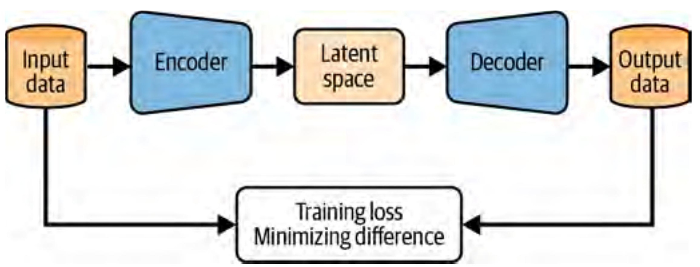
2. AutoEncoder: The Bottleneck Idea
An AutoEncoder is two neural networks stitched together:
- Encoder \(E_\phi\): maps the input \(x\) to a compact latent vector \(z = E_\phi(x)\)
- Decoder \(D_\theta\): reconstructs the input from the latent vector: \(\hat{x} = D_\theta(z)\)
The only training signal: make \(\hat{x}\) look like \(x\). No labels. No external supervision. The pressure to reconstruct faithfully forces the encoder to keep what matters and discard the rest.
$$\mathbf{L}_\text{AE} = \frac{1}{N} \sum_{i=1}^N \| x_i {-} D_\theta(E_\phi(x_i)) \|^2$$
For MNIST digits, the encoder is four convolutional layers that progressively halve the spatial resolution (28→14→7→4→2) while doubling the channel count. A final linear layer projects to the latent dimension. The decoder mirrors this with transposed convolutions. The bottleneck: 784 inputs → 16 latent numbers. A 49× compression.
Training for 10 epochs with MSE loss on a free GPU:
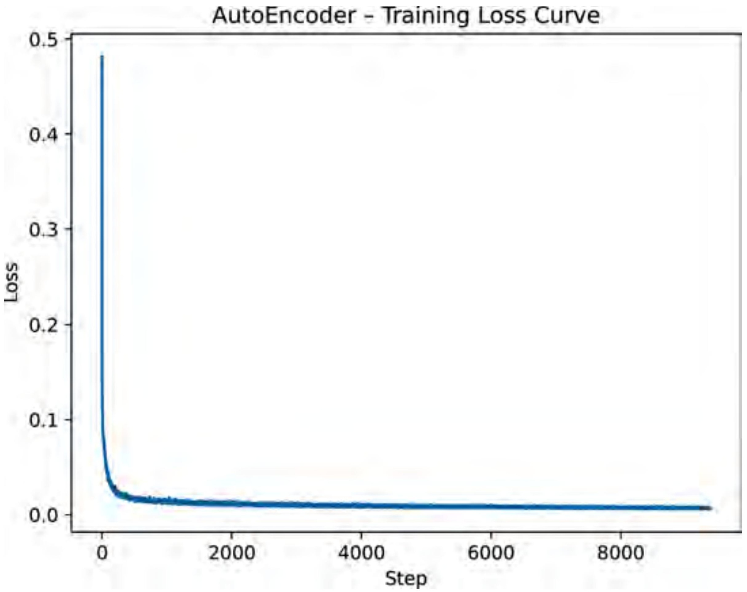
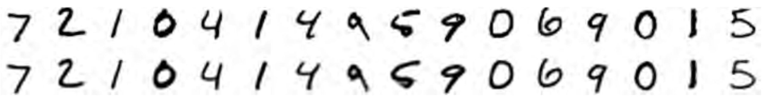
The reconstructions are impressive. 16 numbers turns out to be enough:
3. Visualising the Latent Space
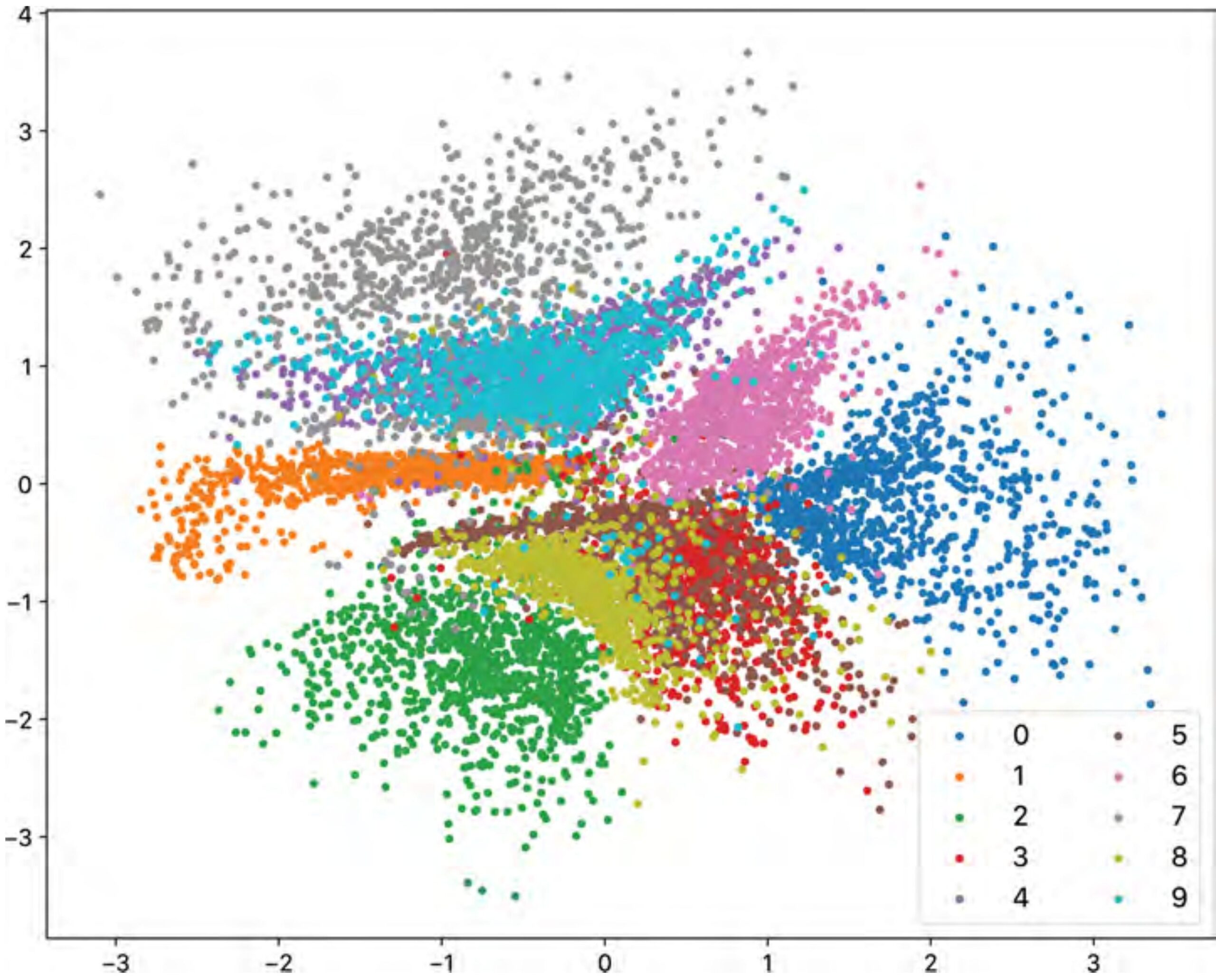
To build intuition, we can train an AutoEncoder with two latent dimensions. Now each input image maps to a single point in a 2D plane, and we can plot all 10,000 test images at once.
The result is one of the most satisfying plots in machine learning:
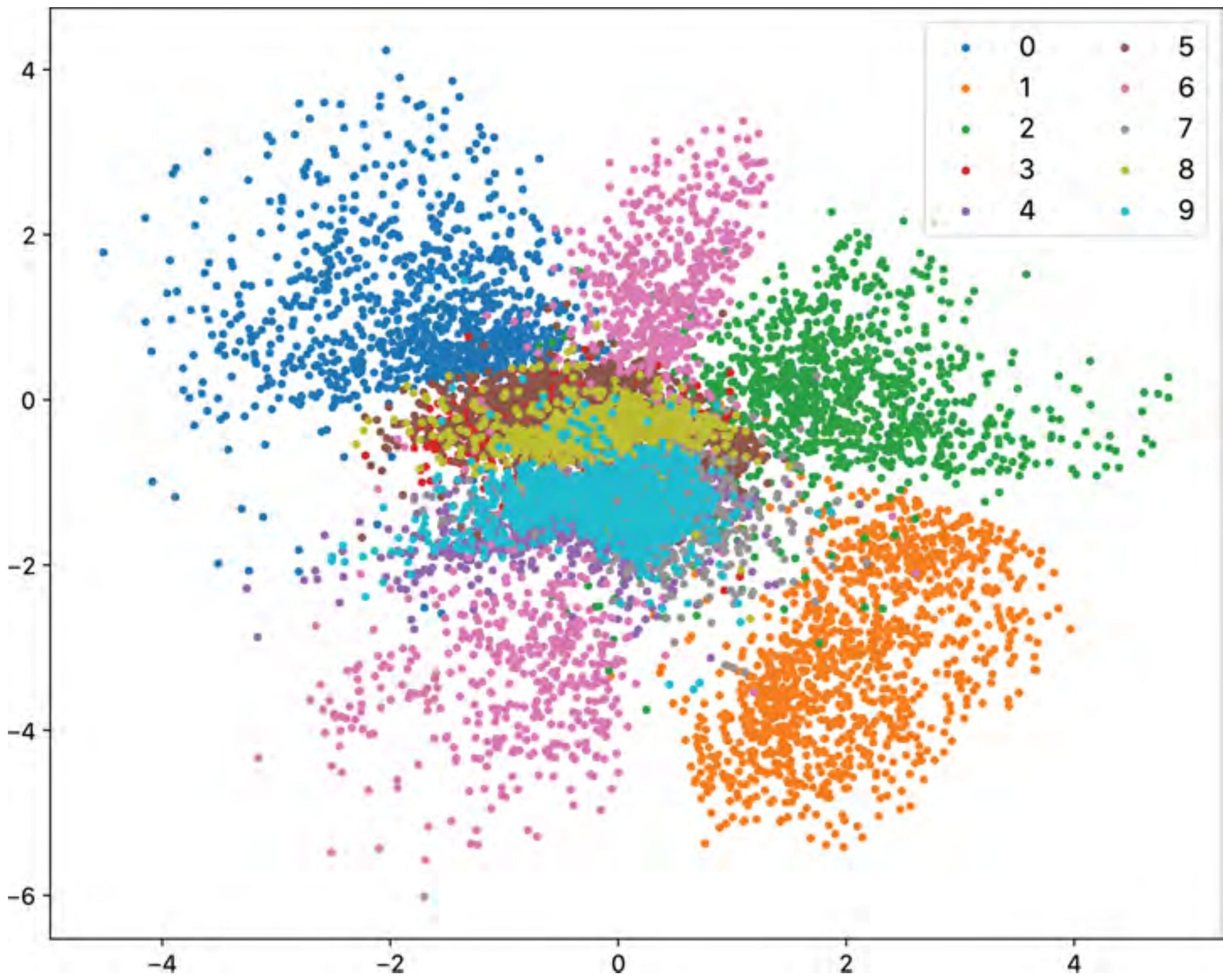
The network has learned, without any supervision, that digit identity is the primary source of variation in this data. This is the manifold the data lives on — the 2D AutoEncoder has found it.
4. Why AutoEncoders Are Bad Generators
Now try to generate a new digit. Sample a random 2D point and decode it.
This usually produces garbage.
The problem is visible in Figure 5. The clusters are irregular. There are gaps between them. The space is asymmetric. If your random sample lands in the void between the “3” cluster and the “8” cluster, the decoder has never been trained to handle that point. It will output something incoherent — because during training, it only ever saw points that actual digits mapped to.
More precisely: the AutoEncoder has learned a good encoder and a good decoder, but it has placed no constraints on the shape of the latent space. The encoder can scatter points anywhere it likes, as long as the decoder can find them again. The result is a “lookup table” — excellent for retrieval, useless for sampling.
The core issue: AutoEncoders compress well but generate poorly. The latent space is not designed to be sampled — only to be decoded from points that the encoder already produced.
| Property | AutoEncoder |
|---|---|
| Reconstruction quality | ✓ Good |
| Latent space structure | ✗ Arbitrary |
| Random sampling | ✗ Unreliable |
| Interpolation | ✗ May hit dead zones |
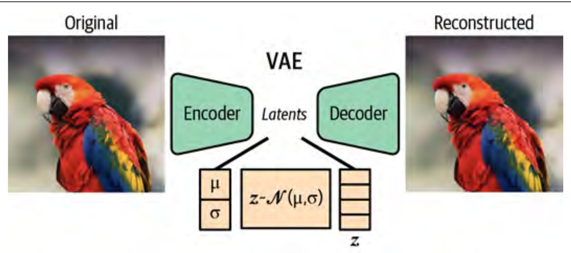
5. VAE: Adding a Distribution to the Bottleneck
The VAE (Kingma & Welling, 2013) fixes this with one conceptual move. Instead of mapping each input to a point \(z\), map it to a probability distribution — specifically a Gaussian parameterised by mean \(\mu\) and log-variance \(\log \sigma^2\):
$$E_\phi(x) \to (\mu, \log \sigma^2)$$
During training, we sample a latent point from this distribution:
$$z \sim \mathbf{N}(\mu, \sigma^2)$$
and pass it to the decoder.
The reparameterization trick. There is a problem: sampling is not differentiable. If \(z \sim \mathbf{N}(\mu, \sigma^2)\), gradients cannot flow back through the sampling step. The fix: write
$$z = \mu + \sigma \cdot \varepsilon, \quad \varepsilon \sim \mathbf{N}(0, I)$$
Now the randomness \(\varepsilon\) is outside the computation graph. The gradients flow through \(\mu\) and \(\sigma\) as usual. This is the reparameterization trick, and it is what makes VAE training tractable.
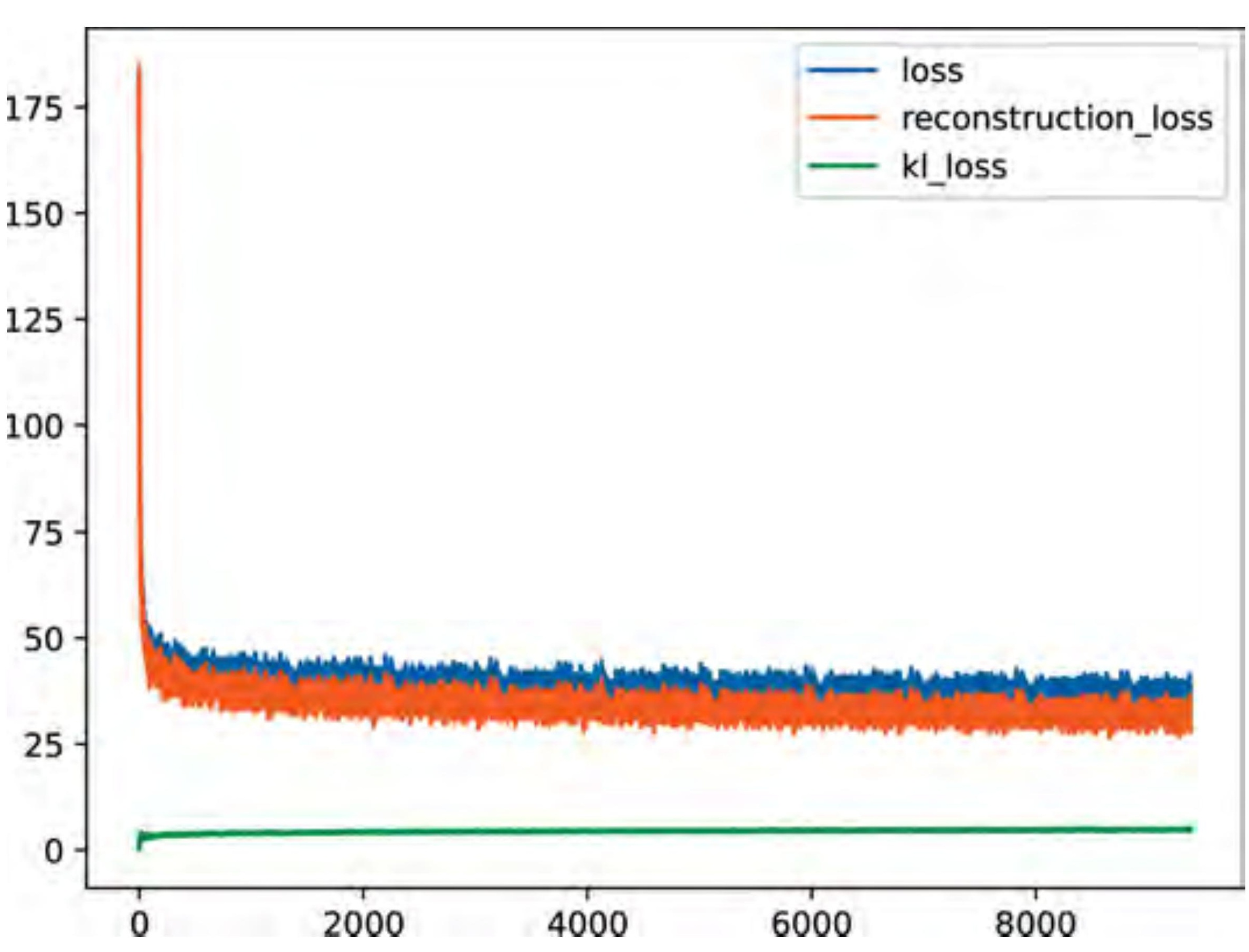
6. The Loss Function: A Tug-of-War
The VAE loss has two terms:
$$\mathbf{L}_\text{VAE} = \underbrace{\mathbf{E}[\| x {-} \hat{x} \|^2]}_{\text{reconstruction}} + \beta \cdot \underbrace{D_\text{KL}\!\left(N(\mu, \sigma^2) \,\|\, \mathbf{N}(0, I)\right)}_{\text{regularisation}}$$
The reconstruction term is the same MSE as before — make \(\hat{x}\) look like \(x\).
The KL divergence term pushes the encoder’s distributions toward the standard Gaussian \(\mathbf{N}(0, I)\). It penalises the encoder for placing distributions far from the origin, or for making them too narrow (which would collapse the stochasticity and reduce the VAE back to an AutoEncoder).
These two terms are in direct tension:
- The reconstruction term wants the encoder to be precise — map each image to a tight, specific distribution so the decoder can reconstruct it accurately.
- The KL term wants the encoder to be vague — keep all distributions close to \(\mathbf{N}(0, I)\) so the latent space is smooth and uniformly covered.
The network finds an equilibrium. Clusters form, but they are pushed toward the origin and forced to overlap slightly. The dead zones disappear.
The hyperparameter \(\beta\) controls the balance. The standard VAE uses \(\beta = 1\). The \(\beta\)-VAE (Higgins et al., 2017) uses \(\beta > 1\) to encourage more disentangled representations — at the cost of some reconstruction quality. For the face experiments below, we use \(\beta = 0.5\) to give the decoder a little more freedom.
7. Comparing the Two Latent Spaces
The payoff of the KL regularisation is visible immediately:
But the most convincing demonstration is the decoded grid. Take a 20×20 uniform grid of points spanning the latent space and decode each one:
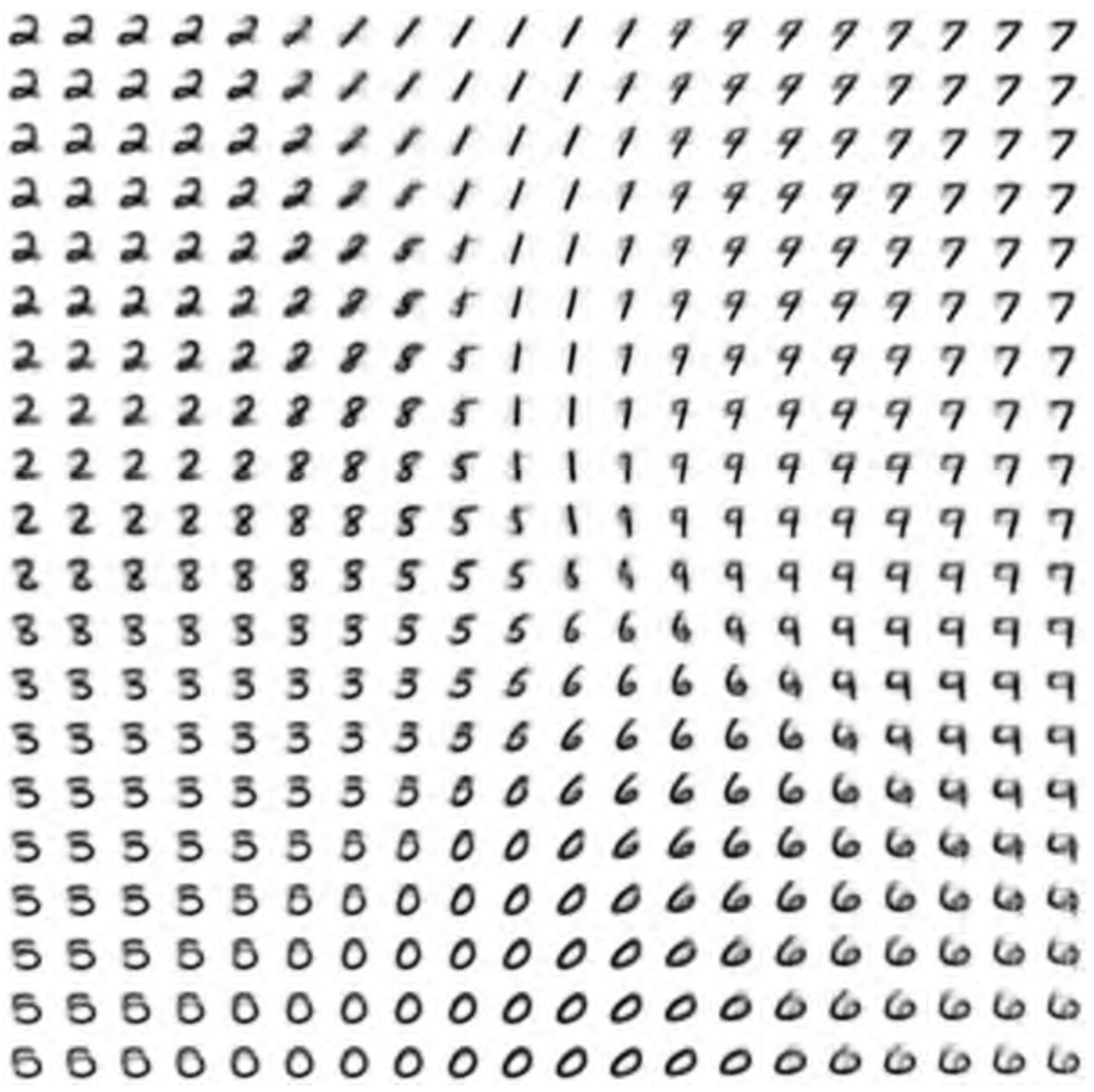
There are no garbage regions. The entire space is valid territory for sampling. This is the property that makes VAEs the preferred encoder/decoder choice inside diffusion models.
| Property | AutoEncoder | VAE |
|---|---|---|
| Reconstruction quality | ✓ Good | ✓ Good (slightly softer) |
| Latent space structure | ✗ Arbitrary | ✓ Gaussian-shaped |
| Random sampling | ✗ Unreliable | ✓ Works by design |
| Smooth interpolation | ✗ May fail | ✓ Guaranteed |
| Used inside Stable Diffusion | ✗ | ✓ |
8. Scaling Up: Face VAE on CelebA
MNIST digits are 28×28 grayscale. Let’s see if the same principles hold on something much harder: 20,000 celebrity face images from CelebA (available on HuggingFace, no authentication required).
The compression challenge is now severe: 12,288 pixel values → 128 latent numbers. A 96× compression ratio.
The architecture scales up to match: four convolutional layers with batch normalisation, 64×64 RGB input, \(\text{LATENT\_DIM} = 128\). Training for 20 epochs on a T4 GPU takes about 7 minutes.
IMG_SIZE    = 64
LATENT_DIM  = 128
BATCH_SIZE  = 128
EPOCHS      = 20
LR          = 1e-3
KL_WEIGHT   = 0.5     # beta-VAE: slightly relax KL to help reconstruction
NUM_TRAIN   = 20_000
Reconstructions. The outputs are blurry. This is not a bug — it is a known limitation of MSE-trained VAEs. MSE penalises pixel-level error uniformly, so the model hedges when uncertain about fine texture, outputting an average. GANs and diffusion models address this with perceptual losses that care about structure, not individual pixels.
Despite the blurriness, every face is recognisable. Face structure, hair colour, skin tone, and pose all survive 96× compression:
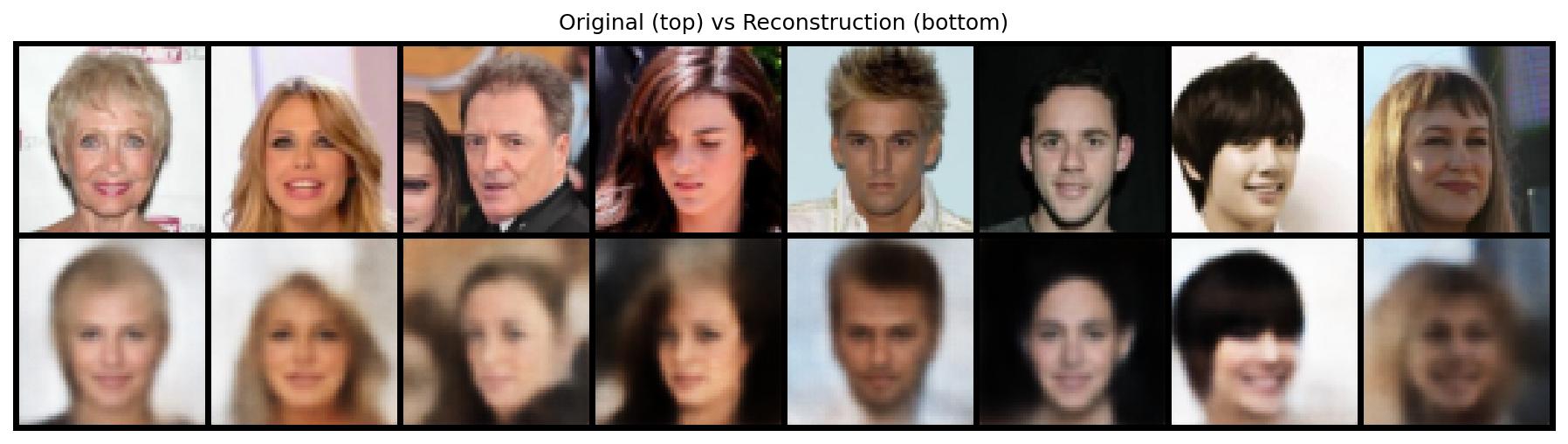
Why blurry? MSE-based reconstruction averages over uncertainty. When the decoder is unsure whether a pixel should be 180 or 200, it outputs 190. Multiply this averaging effect across thousands of pixels and you get a blurry face. Diffusion models, by contrast, learn to sample from the distribution over possible details rather than averaging them out.
9. Random Sampling and Interpolation
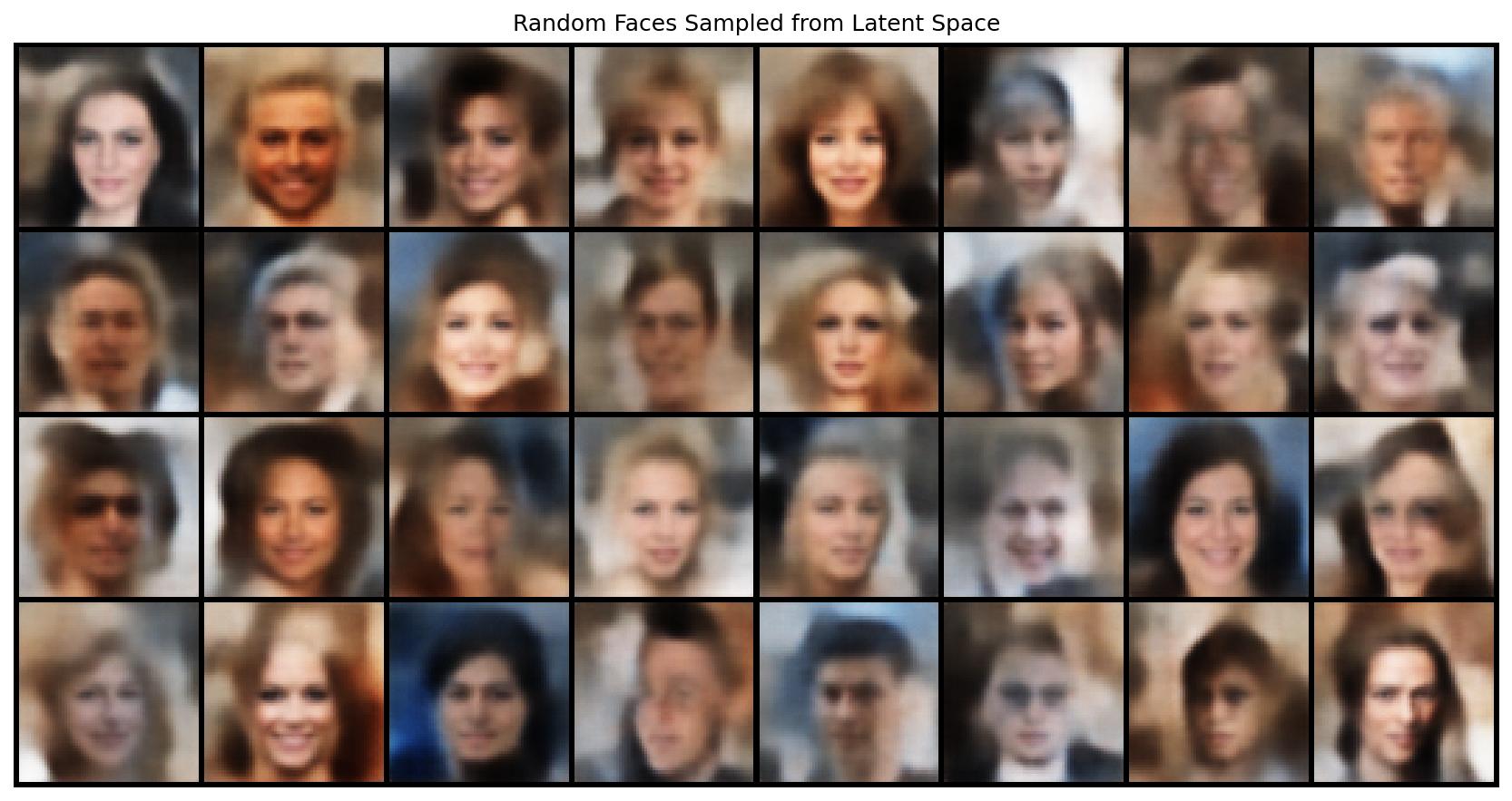
Generating new faces. Sample 32 random vectors from \(\mathbf{N}(0, I)\) in 128 dimensions. Decode each one:
Different genders, hair colours, skin tones, and poses all emerge from random Gaussian samples. The decoder has learned to map the entire standard Gaussian to plausible face space.
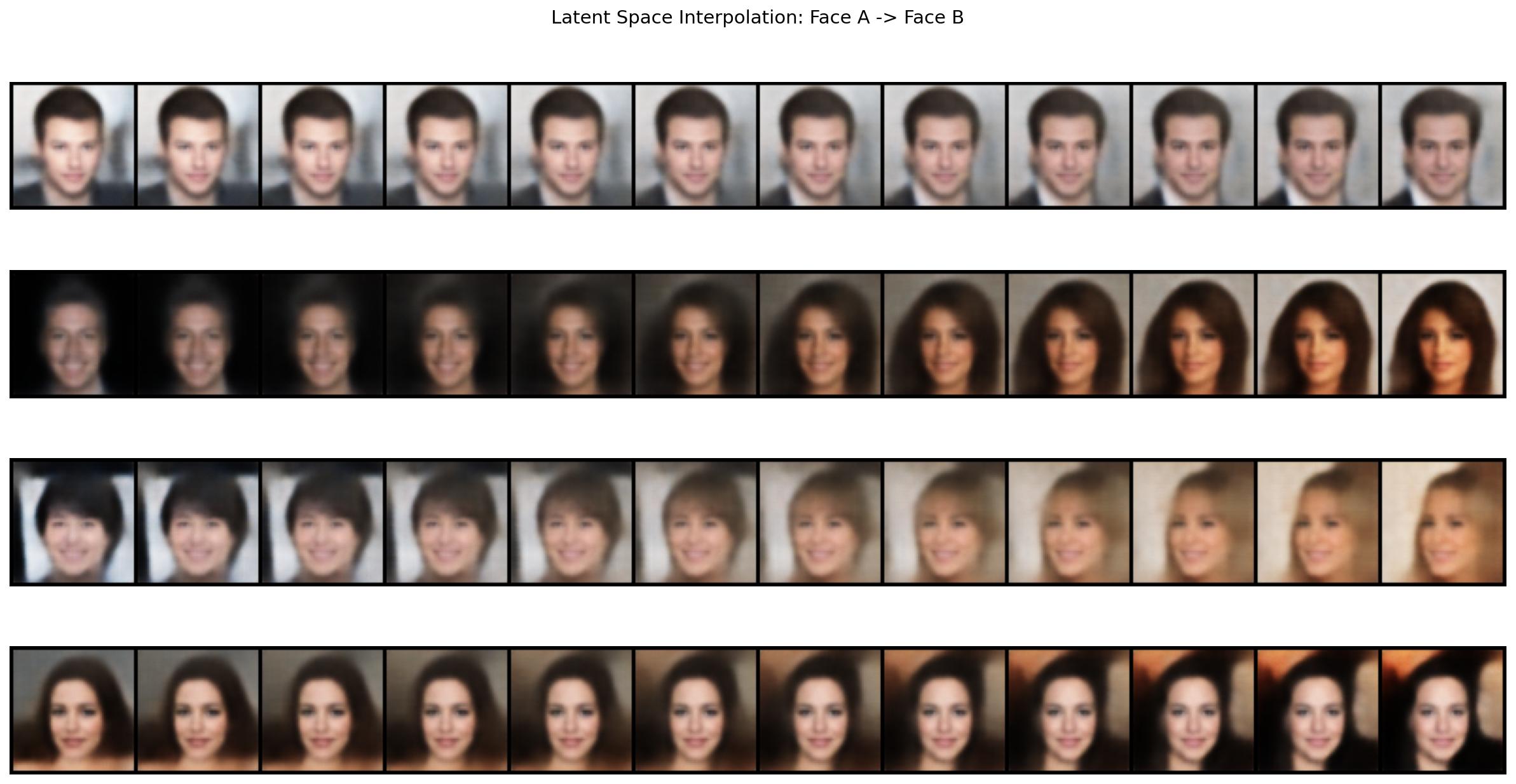
Interpolation. Take two real faces, encode them to latent vectors \(z_A\) and \(z_B\), walk linearly between them, decode each step:
$$z_\alpha = (1 {-} \alpha) z_A + \alpha z_B, \quad \alpha \in [0, 1]$$
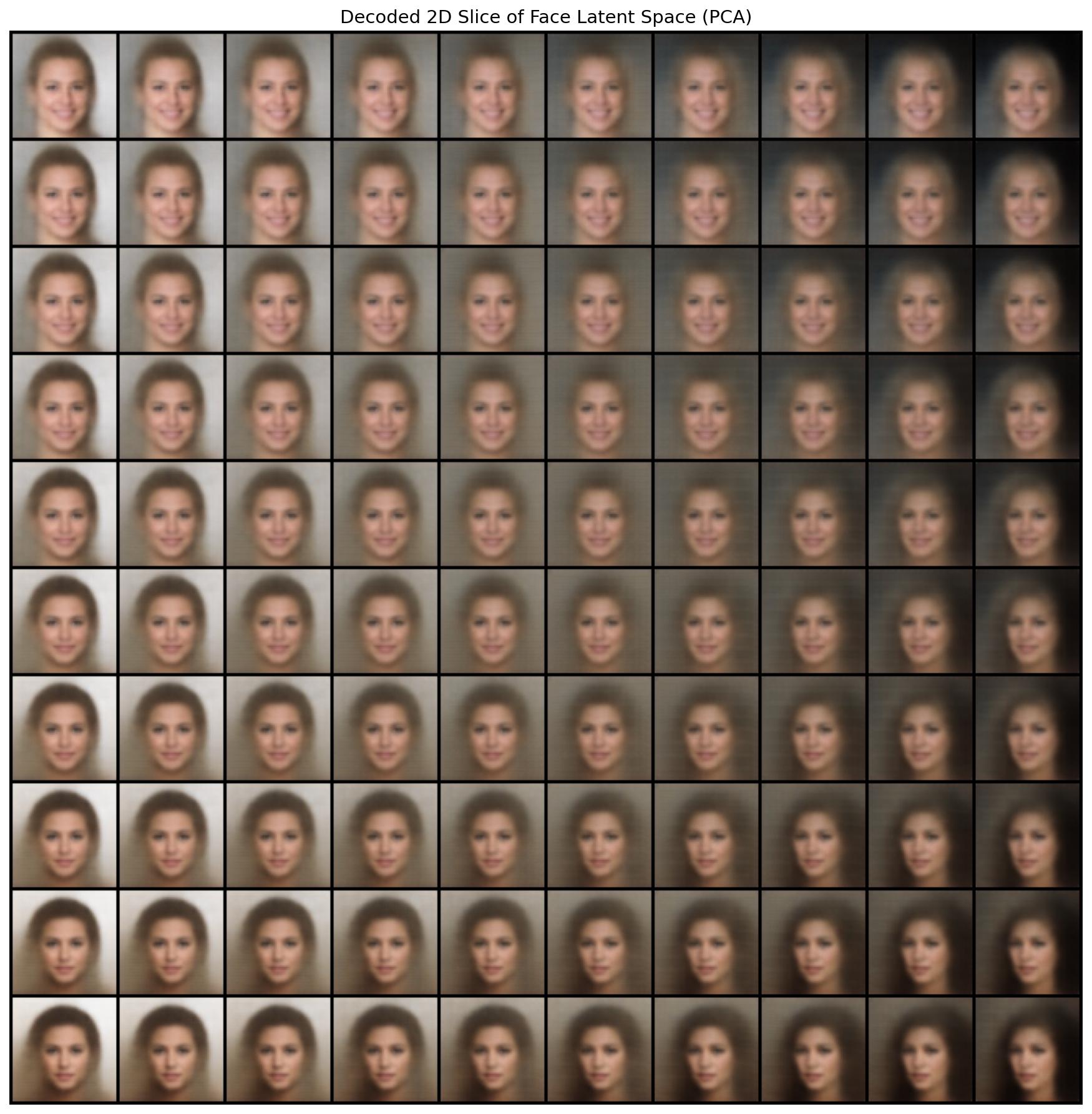
The face manifold. Use PCA to find the two principal directions of variation across all 20,000 latent codes. Decode a 10×10 grid spanning that plane:
10. Are VAEs Dead? Where They Live Today
Fair question. VAEs were introduced in 2013. GANs arrived in 2014 and produced far sharper images. Diffusion models arrived around 2020 and beat GANs on almost every metric. So are VAEs obsolete?
No. They went from being the generative model to being the infrastructure that every other generative model depends on.
The pivot happened with the Latent Diffusion Model paper (Rombach et al., 2022) — the architecture behind Stable Diffusion. The key insight: diffusion is expensive at high resolution because it operates in pixel space. Solution: compress the image first with a VAE, run the diffusion process entirely in the latent space, decode back to pixels at the very end.
Stable Diffusion’s VAE (the kl-f8 encoder) compresses a 512×512 RGB image into a 64×64×4 latent tensor — a spatial 8× reduction plus 4 channels instead of 3. That is the space where all the denoising happens. The VAE is never the creative model — it is the codec. Without it, training and inference at 512×512 would require roughly 64× more computation.
This pattern has held for every major model since:
| Model | VAE role |
|---|---|
| Stable Diffusion 1/2 | kl-f8 encoder/decoder around the UNet |
| SDXL | Improved kl-f8 fine-tuned on LAION-Aesthetics |
| Stable Diffusion 3 / FLUX | New higher-capacity VAE (f8 to f16 experiments) |
| Sora (OpenAI) | Video VAE — spatial + temporal compression |
| CogVideoX | 3D causal VAE for video generation |
| HunyuanVideo | Custom video VAE with spatial+temporal compression |
The research frontier is now about making VAEs better, not replacing them. Active areas as of 2025:
- Video VAEs. Images are one thing; video adds a time dimension. CogVideoX, OpenSora, HunyuanVideo all train 3D causal VAEs that compress both spatially and temporally. The design challenge: temporal compression that does not introduce flickering between frames.
- Diffusability. Recent work (e.g., LiteVAE at NeurIPS 2024, “Improving the Diffusability of Autoencoders” 2025) asks not just whether the VAE reconstructs well, but whether its latent space is structured in a way that makes diffusion training faster and more stable. It turns out that standard KL regularisation does not optimise for this — there is active work on spectral properties of VAE latent spaces.
- Beyond VAEs entirely? A 2025 paper (SVG — latent diffusion without VAE) proposes replacing the VAE with self-supervised vision model features (DINOv2-style), arguing that VAE latent spaces lack semantic structure. The results are interesting, but VAE-based pipelines remain the dominant standard.
Bottom line: The original VAE as a standalone generative model is indeed superseded — you would not train a VAE to generate images anymore, because diffusion models are simply better. But as a compression codec sitting around a diffusion or flow-matching model, the VAE is more central to the field than ever. Every image or video generation model you use today runs inside a VAE’s latent space.
The blurriness problem that seemed like VAEs’ fatal flaw turned out not to matter — because the part that matters (reconstruction quality) was solved by training the decoder with perceptual losses (LPIPS) and adversarial discriminators, and because the generative quality became the diffusion model’s job anyway.
11. Summary
These experiments build a clean progression:
- AutoEncoders prove that neural networks can learn compact, meaningful representations from raw data — no labels needed, just reconstruction pressure.
- VAEs add a probabilistic structure to the latent space via KL regularisation. The resulting space is smooth, centered, and fully sampleable.
- Scaling to faces confirms that the principles hold under 96× compression on real-world images.
- The connection to modern AI: VAEs are not generative models anymore — they are the compression infrastructure inside every major image and video generator. Stable Diffusion, SDXL, FLUX, Sora, HunyuanVideo — all run their diffusion or flow-matching process inside a VAE’s latent space.
Understanding what a latent space is, why the VAE’s Gaussian prior creates one that can be sampled, and how blurriness arises from MSE objectives gives you the conceptual foundation to understand every modern generative system. The code, figures, and training scripts are in the appendix below.
*This post is part of the LLM_log series on datahacker.rs.*
*← LLM_log #012: Diffusion Models — From Noise to Geometry to Sampling | LLM_log #014 →*
Appendix A: Face VAE Training Code
Full training script with all figure generation. Runs on Google Colab (T4 GPU, ~7 min) or locally on Mac (MPS, ~20 min). Uses the CelebA dataset via HuggingFace — no authentication required.
Colab: !pip install -q datasets then paste the script.
Local Mac: pip install datasets then python face_vae_train.py
"""Face VAE — Learning Latent Representations of Faces"""
import os, time, torch, numpy as np
import torch.nn as nn, torch.nn.functional as F
from torch.utils.data import DataLoader, Dataset
from torchvision import transforms
from torchvision.utils import make_grid
import matplotlib.pyplot as plt
# ── Config ───────────────────────────────────────────────────────
IMG_SIZE = 64
LATENT_DIM = 128
BATCH_SIZE = 128 # use 64 for Mac
EPOCHS = 20
LR = 1e-3
KL_WEIGHT = 0.5
NUM_TRAIN = 20_000
FIG_DIR = "/content/figures"
MODEL_PATH = "/content/face_vae.pt"
DEVICE = "cuda" if torch.cuda.is_available() else \
"mps" if torch.backends.mps.is_available() else "cpu"
# ── Data (HuggingFace, no auth) ─────────────────────────────────
class CelebAFaces(Dataset):
def __init__(self, hf_dataset, transform=None):
self.data = hf_dataset
self.transform = transform
def __len__(self):
return len(self.data)
def __getitem__(self, idx):
img = self.data[idx]["image"]
if img.mode != "RGB": img = img.convert("RGB")
return self.transform(img) if self.transform else img
def get_data():
from datasets import load_dataset
hf_ds = load_dataset("nielsr/CelebA-faces", split=f"train[:{NUM_TRAIN}]")
transform = transforms.Compose([
transforms.Resize(IMG_SIZE),
transforms.CenterCrop(IMG_SIZE),
transforms.ToTensor(),
])
dataset = CelebAFaces(hf_ds, transform=transform)
return dataset, DataLoader(dataset, batch_size=BATCH_SIZE,
shuffle=True, num_workers=2, pin_memory=True)
# ── Model ────────────────────────────────────────────────────────
class Encoder(nn.Module):
def __init__(self, latent_dim):
super().__init__()
self.conv = nn.Sequential(
nn.Conv2d(3, 32, 4, 2, 1), nn.BatchNorm2d(32), nn.ReLU(),
nn.Conv2d(32, 64, 4, 2, 1), nn.BatchNorm2d(64), nn.ReLU(),
nn.Conv2d(64, 128, 4, 2, 1), nn.BatchNorm2d(128), nn.ReLU(),
nn.Conv2d(128, 256, 4, 2, 1),nn.BatchNorm2d(256), nn.ReLU(),
)
self.fc_mu = nn.Linear(256 * 4 * 4, latent_dim)
self.fc_logvar = nn.Linear(256 * 4 * 4, latent_dim)
def forward(self, x):
h = self.conv(x).flatten(1)
return self.fc_mu(h), self.fc_logvar(h)
class Decoder(nn.Module):
def __init__(self, latent_dim):
super().__init__()
self.fc = nn.Linear(latent_dim, 256 * 4 * 4)
self.deconv = nn.Sequential(
nn.ConvTranspose2d(256, 128, 4, 2, 1), nn.BatchNorm2d(128), nn.ReLU(),
nn.ConvTranspose2d(128, 64, 4, 2, 1), nn.BatchNorm2d(64), nn.ReLU(),
nn.ConvTranspose2d(64, 32, 4, 2, 1), nn.BatchNorm2d(32), nn.ReLU(),
nn.ConvTranspose2d(32, 3, 4, 2, 1), nn.Sigmoid(),
)
def forward(self, z):
return self.deconv(self.fc(z).view(-1, 256, 4, 4))
class FaceVAE(nn.Module):
def __init__(self, latent_dim):
super().__init__()
self.encoder = Encoder(latent_dim)
self.decoder = Decoder(latent_dim)
def reparameterize(self, mu, logvar):
return mu + torch.randn_like(mu) * torch.exp(0.5 * logvar)
def forward(self, x):
mu, logvar = self.encoder(x)
z = self.reparameterize(mu, logvar)
return self.decoder(z), mu, logvar
def encode(self, x):
mu, _ = self.encoder(x); return mu
def decode(self, z):
return self.decoder(z)
def vae_loss(recon, x, mu, logvar, kl_weight=1.0):
recon_loss = F.mse_loss(recon, x, reduction="sum") / x.size(0)
kl_loss = -0.5 * torch.sum(1 + logvar - mu.pow(2) - logvar.exp()) / x.size(0)
return recon_loss + kl_weight * kl_loss, recon_loss, kl_loss
# ── Training ─────────────────────────────────────────────────────
def train(model, loader):
optimizer = torch.optim.Adam(model.parameters(), lr=LR)
history = {"total": [], "recon": [], "kl": []}
t0 = time.time()
for epoch in range(1, EPOCHS + 1):
model.train()
ep_t, ep_r, ep_k, n = 0, 0, 0, 0
for x in loader:
x = x.to(DEVICE)
recon, mu, logvar = model(x)
loss, rl, kl = vae_loss(recon, x, mu, logvar, KL_WEIGHT)
optimizer.zero_grad(); loss.backward(); optimizer.step()
ep_t += loss.item(); ep_r += rl.item(); ep_k += kl.item(); n += 1
history["total"].append(ep_t/n)
history["recon"].append(ep_r/n)
history["kl"].append(ep_k/n)
print(f"Epoch {epoch:2d}/{EPOCHS} | Total: {ep_t/n:.2f} "
f"| Recon: {ep_r/n:.2f} | KL: {ep_k/n:.2f} | {time.time()-t0:.0f}s")
return history
# ── Figure Generation ────────────────────────────────────────────
def save_fig(fig, name):
fig.savefig(os.path.join(FIG_DIR, name), dpi=150, bbox_inches="tight")
plt.close(fig)
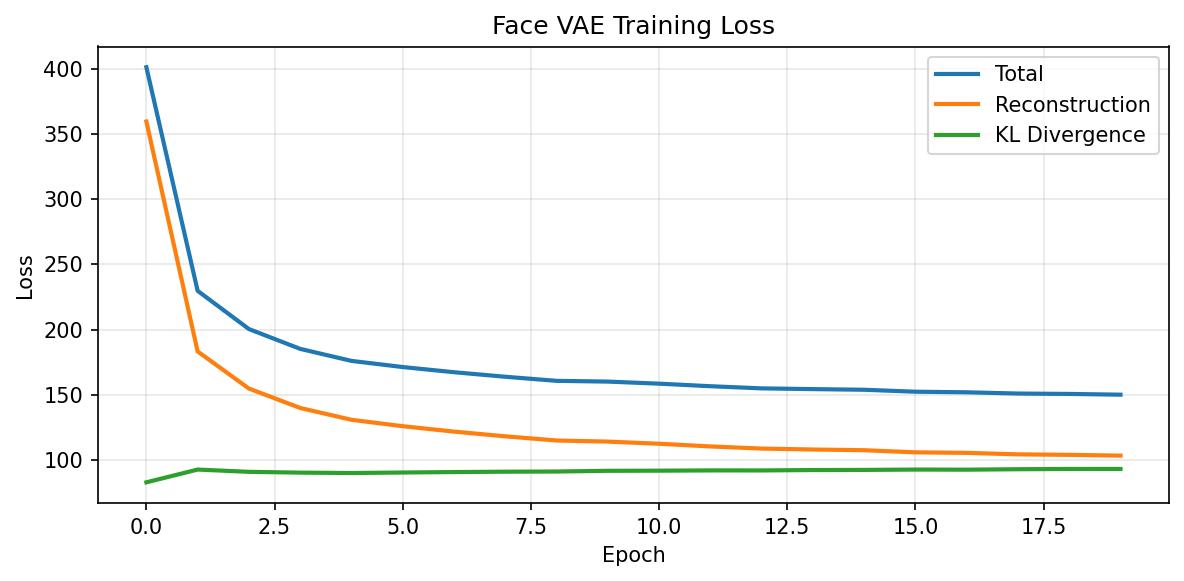
def fig_loss(history):
fig, ax = plt.subplots(figsize=(8, 4))
ax.plot(history["total"], label="Total", lw=2)
ax.plot(history["recon"], label="Reconstruction", lw=2)
ax.plot(history["kl"], label="KL Divergence", lw=2)
ax.set_xlabel("Epoch"); ax.set_ylabel("Loss")
ax.set_title("Face VAE Training Loss"); ax.legend(); ax.grid(True, alpha=0.3)
save_fig(fig, "fig_11_face_vae_training_loss.jpg")
def fig_reconstructions(model, loader):
model.eval()
x = next(iter(loader))[:8].to(DEVICE)
with torch.no_grad(): recon, _, _ = model(x)
grid = make_grid(torch.cat([x.cpu(), recon.cpu()]), nrow=8, padding=2)
fig, ax = plt.subplots(figsize=(14, 3.5))
ax.imshow(grid.permute(1, 2, 0).numpy())
ax.set_title("Original (top) vs Reconstruction (bottom)"); ax.axis("off")
save_fig(fig, "fig_12_face_vae_reconstructions.jpg")
def fig_random_samples(model):
model.eval()
with torch.no_grad():
samples = model.decode(torch.randn(32, LATENT_DIM).to(DEVICE)).cpu()
grid = make_grid(samples, nrow=8, padding=2)
fig, ax = plt.subplots(figsize=(12, 6))
ax.imshow(grid.permute(1, 2, 0).numpy())
ax.set_title("Random Faces Sampled from Latent Space"); ax.axis("off")
save_fig(fig, "fig_13_face_vae_random_samples.jpg")
def fig_interpolation(model, loader, n_pairs=4, n_steps=12):
model.eval()
x = next(iter(loader))[:n_pairs * 2].to(DEVICE)
fig, axes = plt.subplots(n_pairs, 1, figsize=(16, 2.2 * n_pairs))
with torch.no_grad():
for r in range(n_pairs):
z1 = model.encode(x[r*2 : r*2+1])
z2 = model.encode(x[r*2+1 : r*2+2])
alphas = np.linspace(0, 1, n_steps)
interps = [model.decode((1-a)*z1 + a*z2).cpu() for a in alphas]
grid = make_grid(torch.cat(interps), nrow=n_steps, padding=2)
axes[r].imshow(grid.permute(1, 2, 0).numpy()); axes[r].axis("off")
fig.suptitle("Latent Space Interpolation: Face A -> Face B", fontsize=14)
save_fig(fig, "fig_14_face_vae_interpolation.jpg")
def fig_latent_grid(model, loader, grid_size=10):
"""Decode a 2D grid from the PCA principal plane of the latent space."""
model.eval()
all_z = []
with torch.no_grad():
for x in loader:
all_z.append(model.encode(x.to(DEVICE)).cpu())
if sum(len(z) for z in all_z) >= 5000: break
all_z = torch.cat(all_z)
z_mean = all_z.mean(0)
_, _, V = torch.pca_lowrank(all_z - z_mean, q=2)
vals = np.linspace(-3, 3, grid_size)
faces = []
with torch.no_grad():
for y in vals:
for xv in vals:
z = z_mean + xv * V[:, 0] + y * V[:, 1]
faces.append(model.decode(z.unsqueeze(0).to(DEVICE)).cpu())
grid = make_grid(torch.cat(faces), nrow=grid_size, padding=2)
fig, ax = plt.subplots(figsize=(12, 12))
ax.imshow(grid.permute(1, 2, 0).numpy())
ax.set_title("Decoded 2D Slice of Face Latent Space (PCA)", fontsize=14)
ax.axis("off")
save_fig(fig, "fig_15_face_vae_latent_grid.jpg")
# ── Main ─────────────────────────────────────────────────────────
if __name__ == "__main__":
os.makedirs(FIG_DIR, exist_ok=True)
dataset, loader = get_data()
model = FaceVAE(LATENT_DIM).to(DEVICE)
history = train(model, loader)
torch.save(model.state_dict(), MODEL_PATH)
fig_loss(history)
fig_reconstructions(model, loader)
fig_random_samples(model)
fig_interpolation(model, loader)
fig_latent_grid(model, loader)
Appendix B: Figure Extraction Pipeline
Figures fig_01 through fig_10 were extracted from the source PDF using a DocLayout-YOLO model. The pipeline converts PDF pages to high-res images at 600 DPI, runs YOLO detection to locate figure zones, and crops them out.
# config.py — Pipeline configuration
from pathlib import Path

BASE_DIR = Path(__file__).parent.resolve()
PDF_PATH = BASE_DIR / "Latent_013.pdf"
PDF_CROPS_DIR = BASE_DIR / "pdf_crops"
ANNOTATED_PAGES_DIR = BASE_DIR / "annotated_pages"
ACCEPTED_FIGURES_DIR = BASE_DIR / "accepted_figures"
YOLO_MODEL_PATH = BASE_DIR / "doclayout_yolo_docstructbench_imgsz1024.pt"

PDF_DPI = 600
YOLO_CONF_THRESHOLD = 0.2
YOLO_IMGSZ = 1024
EXTRACT_LABELS = ["figure"]
MAX_FIGURES = None
# exp_001_extraction.py — Figure extraction from PDF
# Converts PDF pages to images (600 DPI), runs DocLayout-YOLO to detect
# figure zones, crops and saves them, and produces annotated page overlays.
# Usage: python exp_001_extraction.py
# Requires: pdf2image, doclayout_yolo, opencv-python
# See full source in the repository.
Appendix C: MNIST AutoEncoder & VAE Training Code
Generates fig_01 through fig_09. Runs on Google Colab (CPU or free GPU, ~5 min) or locally. No external datasets needed — MNIST downloads automatically via torchvision.
Colab: Runtime → Run all. No extra installs needed.
Local: python mnist_ae_vae.py
"""
MNIST AutoEncoder + VAE — Latent Space Experiments
Generates: fig_02 to fig_09 (architecture figures fig_01 are hand-drawn)
Colab: Runtime > Run all  |  Local: python mnist_ae_vae.py
!pip install torch torchvision matplotlib scikit-learn  # if needed
"""
import os
import torch
import torch.nn as nn
import torch.nn.functional as F
from torch.utils.data import DataLoader
from torchvision import datasets, transforms
from torchvision.utils import make_grid
import matplotlib.pyplot as plt
import matplotlib.gridspec as gridspec
import numpy as np

# ── Config ────────────────────────────────────────────────────────
LATENT_DIM_MAIN = 16       # main AE/VAE latent dim for reconstructions
LATENT_DIM_2D   = 2        # 2D latent dim for visualisation
BATCH_SIZE      = 256
EPOCHS_MAIN     = 10
EPOCHS_2D       = 20       # 2D models need more epochs to separate clusters
LR              = 1e-3
FIG_DIR         = "figures"
DEVICE          = "cuda" if torch.cuda.is_available() else "cpu"

os.makedirs(FIG_DIR, exist_ok=True)

# ── Data ──────────────────────────────────────────────────────────
transform = transforms.ToTensor()
train_ds = datasets.MNIST(".", train=True,  download=True, transform=transform)
test_ds  = datasets.MNIST(".", train=False, download=True, transform=transform)
train_loader = DataLoader(train_ds, batch_size=BATCH_SIZE, shuffle=True,  num_workers=2)
test_loader  = DataLoader(test_ds,  batch_size=BATCH_SIZE, shuffle=False, num_workers=2)

# ── AutoEncoder ───────────────────────────────────────────────────
class AEEncoder(nn.Module):
    def __init__(self, latent_dim):
        super().__init__()
        self.conv = nn.Sequential(
            nn.Conv2d(1, 32, 4, 2, 1),   nn.ReLU(),   # 28→14
            nn.Conv2d(32, 64, 4, 2, 1),  nn.ReLU(),   # 14→7
            nn.Conv2d(64, 128, 3, 2, 1), nn.ReLU(),   # 7→4
            nn.Conv2d(128, 64, 3, 2, 1), nn.ReLU(),   # 4→2
        )
        self.fc = nn.Linear(64 * 2 * 2, latent_dim)

    def forward(self, x):
        return self.fc(self.conv(x).flatten(1))

class AEDecoder(nn.Module):
    def __init__(self, latent_dim):
        super().__init__()
        self.fc = nn.Linear(latent_dim, 64 * 2 * 2)
        self.deconv = nn.Sequential(
            nn.ConvTranspose2d(64, 128, 3, 2, 1, output_padding=1), nn.ReLU(),  # 2→4
            nn.ConvTranspose2d(128, 64, 3, 2, 1, output_padding=0), nn.ReLU(),  # 4→7
            nn.ConvTranspose2d(64, 32, 4, 2, 1, output_padding=0),  nn.ReLU(),  # 7→14
            nn.ConvTranspose2d(32, 1, 4, 2, 1),  nn.Sigmoid(),                  # 14→28
        )

    def forward(self, z):
        return self.deconv(self.fc(z).view(-1, 64, 2, 2))

class AutoEncoder(nn.Module):
    def __init__(self, latent_dim):
        super().__init__()
        self.encoder = AEEncoder(latent_dim)
        self.decoder = AEDecoder(latent_dim)

    def forward(self, x):
        return self.decoder(self.encoder(x))

    def encode(self, x):
        return self.encoder(x)

    def decode(self, z):
        return self.decoder(z)

# ── VAE ───────────────────────────────────────────────────────────
class VAEEncoder(nn.Module):
    def __init__(self, latent_dim):
        super().__init__()
        self.conv = nn.Sequential(
            nn.Conv2d(1, 32, 4, 2, 1),   nn.ReLU(),
            nn.Conv2d(32, 64, 4, 2, 1),  nn.ReLU(),
            nn.Conv2d(64, 128, 3, 2, 1), nn.ReLU(),
            nn.Conv2d(128, 64, 3, 2, 1), nn.ReLU(),
        )
        self.fc_mu     = nn.Linear(64 * 2 * 2, latent_dim)
        self.fc_logvar = nn.Linear(64 * 2 * 2, latent_dim)

    def forward(self, x):
        h = self.conv(x).flatten(1)
        return self.fc_mu(h), self.fc_logvar(h)

class VAE(nn.Module):
    def __init__(self, latent_dim):
        super().__init__()
        self.encoder = VAEEncoder(latent_dim)
        self.decoder = AEDecoder(latent_dim)   # same decoder as AE

    def reparameterize(self, mu, logvar):
        return mu + torch.randn_like(mu) * torch.exp(0.5 * logvar)

    def forward(self, x):
        mu, logvar = self.encoder(x)
        z = self.reparameterize(mu, logvar)
        return self.decoder(z), mu, logvar

    def encode(self, x):
        mu, _ = self.encoder(x)
        return mu

    def decode(self, z):
        return self.decoder(z)

# ── Loss functions ────────────────────────────────────────────────
def ae_loss(recon, x):
    return F.mse_loss(recon, x, reduction="sum") / x.size(0)

def vae_loss(recon, x, mu, logvar):
    recon_loss = F.mse_loss(recon, x, reduction="sum") / x.size(0)
    kl_loss    = -0.5 * torch.sum(1 + logvar - mu.pow(2) - logvar.exp()) / x.size(0)
    return recon_loss + kl_loss, recon_loss, kl_loss

# ── Training ──────────────────────────────────────────────────────
def train_ae(model, loader, epochs):
    opt = torch.optim.Adam(model.parameters(), lr=LR)
    history = []
    for ep in range(1, epochs + 1):
        model.train()
        total = 0
        for x, _ in loader:
            x = x.to(DEVICE)
            loss = ae_loss(model(x), x)
            opt.zero_grad(); loss.backward(); opt.step()
            total += loss.item()
        avg = total / len(loader)
        history.append(avg)
        print(f"AE Epoch {ep:2d}/{epochs} | Loss: {avg:.4f}")
    return history

def train_vae(model, loader, epochs):
    opt = torch.optim.Adam(model.parameters(), lr=LR)
    history = {"total": [], "recon": [], "kl": []}
    for ep in range(1, epochs + 1):
        model.train()
        t, r, k = 0, 0, 0
        for x, _ in loader:
            x = x.to(DEVICE)
            recon, mu, logvar = model(x)
            loss, rl, kl = vae_loss(recon, x, mu, logvar)
            opt.zero_grad(); loss.backward(); opt.step()
            t += loss.item(); r += rl.item(); k += kl.item()
        n = len(loader)
        history["total"].append(t/n); history["recon"].append(r/n); history["kl"].append(k/n)
        print(f"VAE Epoch {ep:2d}/{epochs} | Total: {t/n:.2f} | Recon: {r/n:.2f} | KL: {k/n:.2f}")
    return history

# ── Figure helpers ────────────────────────────────────────────────
def save_fig(fig, name):
    fig.savefig(os.path.join(FIG_DIR, name), dpi=150, bbox_inches="tight")
    plt.close(fig)

def fig_ae_loss(history, name):
    fig, ax = plt.subplots(figsize=(8, 4))
    ax.plot(history, lw=2, color="#2196f3")
    ax.set_xlabel("Epoch"); ax.set_ylabel("MSE Loss")
    ax.set_title("AutoEncoder Training Loss"); ax.grid(True, alpha=0.3)
    save_fig(fig, name)

def fig_vae_loss(history, name):
    fig, ax = plt.subplots(figsize=(8, 4))
    ax.plot(history["total"], label="Total",          lw=2)
    ax.plot(history["recon"], label="Reconstruction", lw=2)
    ax.plot(history["kl"],    label="KL Divergence",  lw=2)
    ax.set_xlabel("Epoch"); ax.set_ylabel("Loss")
    ax.set_title("VAE Loss Components"); ax.legend(); ax.grid(True, alpha=0.3)
    save_fig(fig, name)

def fig_reconstructions(model, loader, name):
    model.eval()
    x, _ = next(iter(loader))
    x = x[:8].to(DEVICE)
    with torch.no_grad():
        if isinstance(model, VAE):
            recon, _, _ = model(x)
        else:
            recon = model(x)
    grid = make_grid(torch.cat([x.cpu(), recon.cpu()]), nrow=8, padding=2)
    fig, ax = plt.subplots(figsize=(12, 3))
    ax.imshow(grid.permute(1, 2, 0).squeeze().numpy(), cmap="gray")
    ax.set_title("Original (top) vs Reconstruction (bottom)"); ax.axis("off")
    save_fig(fig, name)

def fig_2d_latent(model, loader, name, n_samples=5000):
    model.eval()
    zs, ys = [], []
    with torch.no_grad():
        for x, y in loader:
            z = model.encode(x.to(DEVICE)).cpu().numpy()
            zs.append(z); ys.append(y.numpy())
            if sum(len(a) for a in zs) >= n_samples:
                break
    zs = np.concatenate(zs)[:n_samples]
    ys = np.concatenate(ys)[:n_samples]
    fig, ax = plt.subplots(figsize=(8, 7))
    sc = ax.scatter(zs[:, 0], zs[:, 1], c=ys, cmap="tab10", s=4, alpha=0.6)
    plt.colorbar(sc, ax=ax, ticks=range(10))
    ax.set_xlabel("z[0]"); ax.set_ylabel("z[1]")
    ax.set_title("2D Latent Space"); ax.grid(True, alpha=0.2)
    save_fig(fig, name)

def fig_decoded_grid(model, name, grid_size=20, z_range=3.0):
    """Decode a uniform grid of 2D latent points (VAE only)."""
    model.eval()
    vals = np.linspace(-z_range, z_range, grid_size)
    imgs = []
    with torch.no_grad():
        for y in reversed(vals):          # top row = positive y
            for x in vals:
                z = torch.tensor([[x, y]], dtype=torch.float32).to(DEVICE)
                imgs.append(model.decode(z).cpu())
    grid = make_grid(torch.cat(imgs), nrow=grid_size, padding=1, pad_value=0.5)
    fig, ax = plt.subplots(figsize=(10, 10))
    ax.imshow(grid.permute(1, 2, 0).squeeze().numpy(), cmap="gray")
    ax.set_title(f"VAE Decoded {grid_size}×{grid_size} Latent Grid"); ax.axis("off")
    save_fig(fig, name)

# ── Main ──────────────────────────────────────────────────────────
if __name__ == "__main__":

    # 1. AutoEncoder — 16D (reconstructions + loss)
    print("\n=== AutoEncoder 16D ===")
    ae16 = AutoEncoder(LATENT_DIM_MAIN).to(DEVICE)
    ae16_hist = train_ae(ae16, train_loader, EPOCHS_MAIN)
    fig_ae_loss(ae16_hist,                  "fig_03_ae_training_loss_curve.jpg")
    fig_reconstructions(ae16, test_loader,  "fig_04_ae_reconstruction_16dim.jpg")

    # 2. AutoEncoder — 2D (latent space visualisation)
    print("\n=== AutoEncoder 2D ===")
    ae2 = AutoEncoder(LATENT_DIM_2D).to(DEVICE)
    train_ae(ae2, train_loader, EPOCHS_2D)
    fig_2d_latent(ae2, test_loader, "fig_05_ae_2d_latent_space.jpg")

    # 3. VAE — 16D (loss components)
    print("\n=== VAE 16D ===")
    vae16 = VAE(LATENT_DIM_MAIN).to(DEVICE)
    vae16_hist = train_vae(vae16, train_loader, EPOCHS_MAIN)
    fig_vae_loss(vae16_hist, "fig_07_vae_loss_components.jpg")

    # 4. VAE — 2D (latent space + decoded grid)
    print("\n=== VAE 2D ===")
    vae2 = VAE(LATENT_DIM_2D).to(DEVICE)
    train_vae(vae2, train_loader, EPOCHS_2D)
    fig_2d_latent(vae2, test_loader,   "fig_08_vae_2d_latent_space.jpg")
    fig_decoded_grid(vae2,             "fig_09_vae_decoded_2d_grid.jpg")

    print(f"\nAll figures saved to ./{FIG_DIR}/")