Highlights: In this post, we take a deep dive into the architecture that changed everything — the Transformer — and trace its evolution from NLP into computer vision. We start with the original encoder-decoder model, walk through self-attention and multi-head attention step by step, and then show how Vision Transformers (ViT) apply the exact same mechanism to image patches instead of words. Along the way, we answer the questions that trip everyone up: if we slice an image into patches, how can the model learn anything spatial? And what exactly is the [CLS] token — an empty vector that somehow learns to classify? Finally, we cover the SWIN Transformer, which introduced hierarchical processing and shifted windows to make ViTs practical for detection and segmentation. A companion Colab notebook lets you run all the experiments hands-on.

Tutorial Overview:

1. Transformer Fundamentals
2. Self-Attention: The Core Innovation
3. Multi-Head Attention and the Encoder Block
4. The Decoder and Masked Attention
5. From CNNs to Vision Transformers
6. The ViT Architecture
7. Wait — How Can Patches Learn Spatial Relationships?
8. The [CLS] Token: An Empty Vector That Learns Everything
9. Position Embeddings: 1D Labels, 2D Understanding
10. ViT Performance and Scaling
11. How ViTs See vs. How CNNs See
12. SWIN Transformer: Hierarchical Vision
13. Shifted Windows and the Full SWIN Architecture
14. Hands-On: ViT Experiments (Colab)
15. Key Takeaways
16. Can Pure Vision Models See Wealth?
17. Experiment 6: Centroid Separation
18. Experiment 7: SVM vs Centroid Across Dimensions
19. Experiment 8: How Much Data Do You Need?
20. What We Learned: Vision Models Compared

---

1. Transformer Fundamentals

In 2017, Vaswani et al. published “Attention is All You Need” and introduced the Transformer — an architecture that achieved a new state of the art in machine translation while requiring only a fraction of the training time of previous models. Within a couple of years, Transformers completely displaced RNNs and LSTMs in NLP. By 2020, they started doing the same in computer vision.

Why were Transformers so much better? Two fundamental advantages over RNN-based models. First, Transformers can efficiently learn long-range dependencies — meaningful relationships between tokens that are far apart in a sequence. RNNs struggle with this because information must propagate step-by-step through the hidden state. Second, Transformer training is parallelizable. RNNs are inherently sequential — you can’t compute the hidden state at position t without first computing it at t-1. Transformers process all tokens simultaneously.

The original Transformer has two macro components: an Encoder (left) and a Decoder (right). In machine translation, the Encoder takes a sentence in one language (say French) and compresses it into a latent representation. The Decoder takes that representation and generates the equivalent sentence in another language (say English).

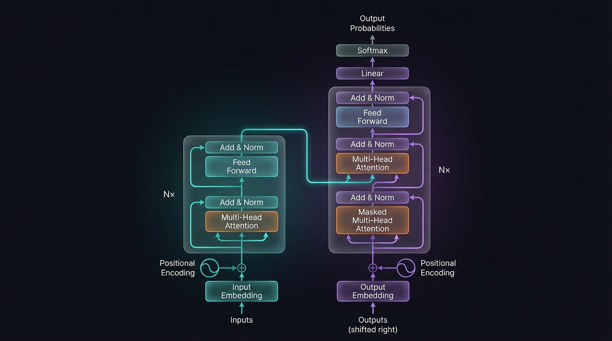
The complete Transformer architecture. Left: the Encoder stack (teal). Right: the Decoder stack (purple). Both use Multi-Head Attention as their core mechanism, but the Decoder adds masked attention and cross-attention layers.

Looking at this diagram, many components are standard deep learning building blocks — Feed Forward networks, Layer Normalization, linear projection, softmax. The key innovation is the Multi-Head Attention mechanism (and its masked variant in the Decoder). As the paper title says: attention is all you need.

On the Encoder side, each input token is embedded into a continuous vector, enriched with positional encoding, and processed through N× repeated blocks. Each block contains Multi-Head Attention → Add & Norm → Feed Forward → Add & Norm. The Decoder mirrors this structure but adds a Masked Multi-Head Attention layer at the bottom and a cross-attention layer that receives the Encoder’s output. At the very top, a Linear layer followed by Softmax produces output probabilities over the vocabulary.

---

2. Self-Attention: The Core Innovation

The heart of the Transformer is the self-attention mechanism. This is what allows every position in a sequence to “look at” every other position in a single computational step — a fundamentally different approach from RNNs, which must process tokens one by one.

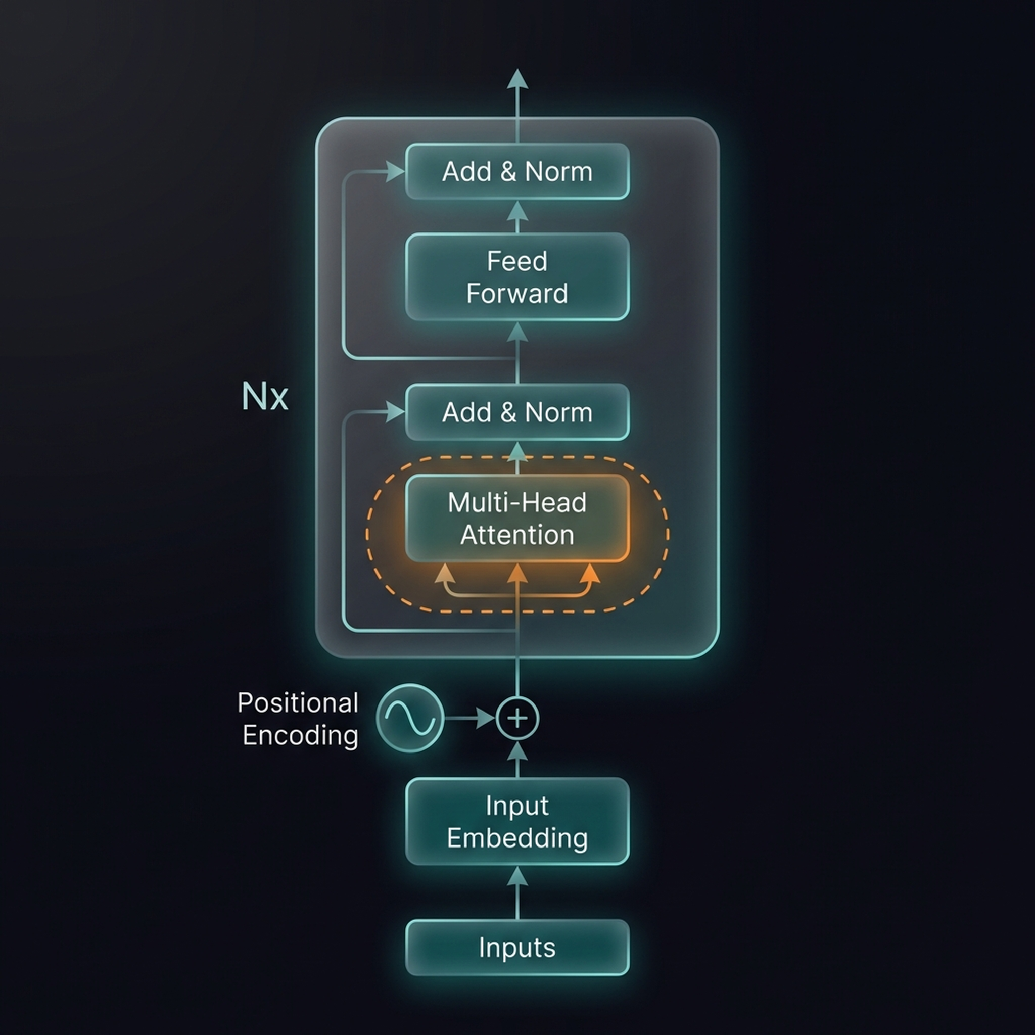
The Encoder structure with the Multi-Head Attention module highlighted (orange dashed border). The three arrows entering the attention block represent the Query (Q), Key (K), and Value (V) projections — all derived from the same input.

Here’s how self-attention works. Starting from the input embedding matrix X (with dimensions [num_tokens, embedding_dim]), we create three separate matrices by multiplying with learned weight matrices:

• Q = X · W_Q (the Query matrix — “what am I looking for?”)
• K = X · W_K (the Key matrix — “what do I contain?”)
• V = X · W_V (the Value matrix — “what information do I carry?”)

The attention output is:

$$\text{Attention}(Q, K, V) = \text{softmax}\left(\frac{Q \cdot K^T}{\sqrt{d_k}}\right) \cdot V$$

The product Q · K^T computes a similarity score between every pair of tokens. Division by √d_k prevents the dot products from growing too large, which would push softmax into saturated regions with tiny gradients. After softmax, each row becomes a probability distribution — the attention weights. Multiplying by V produces the output: a weighted sum of value vectors, where the weights reflect relevance.

The critical insight: a token at position 1 can directly attend to a token at position 100 in a single step. In an RNN, that information would need to survive 99 sequential hidden state updates.

---

3. Multi-Head Attention and the Encoder Block

A single attention head captures one type of relationship between tokens. But language and vision involve multiple types of relationships simultaneously — syntactic, semantic, positional. Multi-Head Attention (MHA) addresses this by running h independent attention heads in parallel, each with its own learned projections.

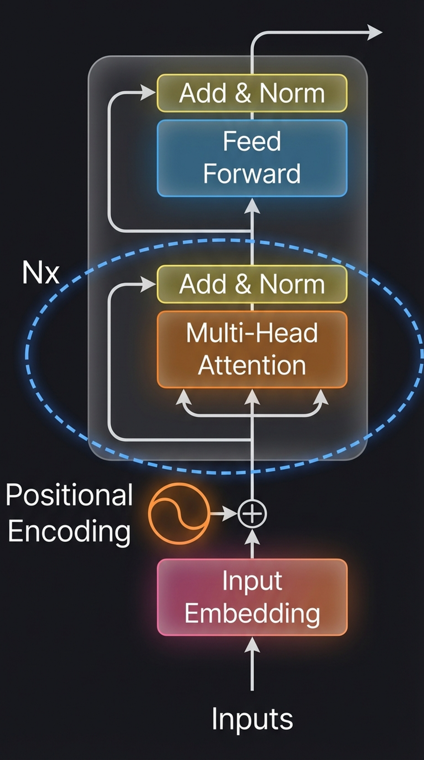
An alternative view of the Encoder block emphasizing the Multi-Head Attention module (orange) with the blue dashed ellipse. The same input is projected three ways (Q, K, V) and processed through multiple heads.

Each head independently computes its own attention, then all outputs are concatenated and projected:

$$\text{MultiHead}(Q, K, V) = \text{Concat}(\text{head}_1, \ldots, \text{head}_h) \cdot W_O$$

In the original Transformer, h = 8 heads operate on 512 / 8 = 64 dimensions each. This is computationally equivalent to single full-dimensional attention, but allows the model to capture multiple relationship types simultaneously. In practice, different heads often specialize — one might focus on local dependencies while another captures long-range structure.

Now let’s see how all the pieces fit together inside a single Encoder block.

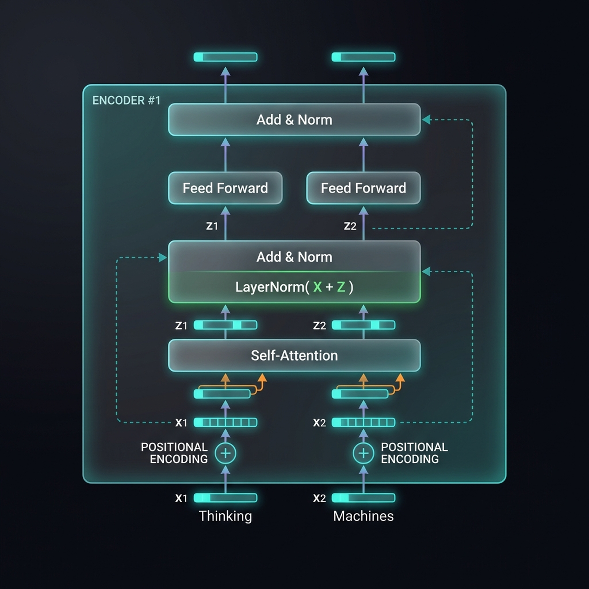
Inside Encoder #1: the words “Thinking” and “Machines” are processed through the full pipeline. After positional encoding (⊕), Self-Attention produces context-aware representations Z1 and Z2. Add & Norm computes LayerNorm(X + Z) — the residual connection. Feed Forward networks process each position independently, followed by another Add & Norm.

The residual connection (X + Z) is crucial — it adds the original input back to the attention output before normalization. This ensures gradient can flow directly through the network and allows the attention layer to learn a refinement of the input rather than a complete replacement. The Feed Forward network (a two-layer MLP with GELU activation) gives the model per-token nonlinear transformation capacity beyond what attention provides.

This entire block is stacked N times (typically N = 6), producing increasingly refined representations.

---

4. The Decoder and Masked Attention

The Decoder has a critical constraint: during training, it must not see future tokens in the target sequence. If it could peek ahead, it would just copy instead of learning to generate.

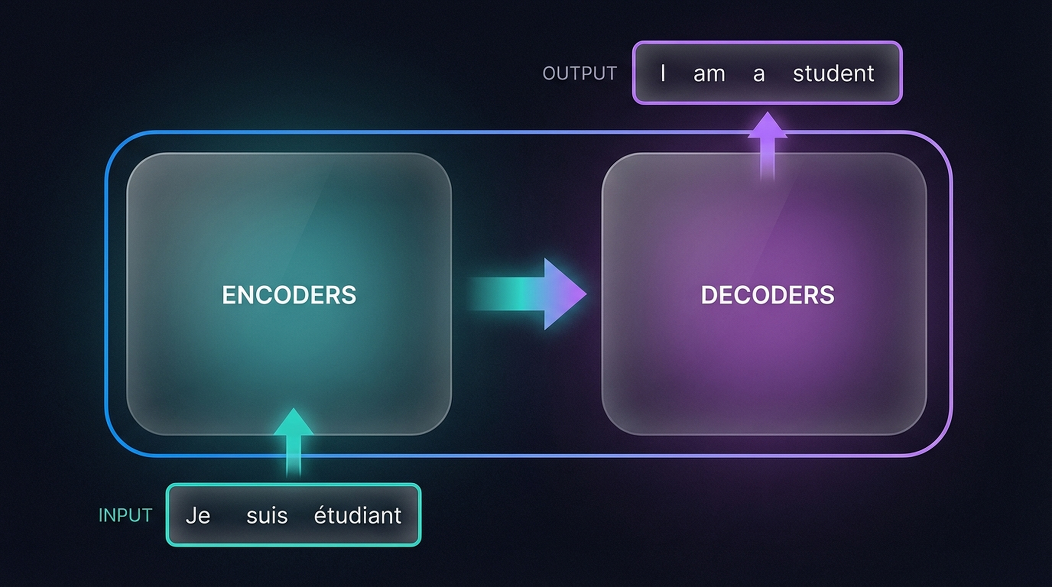
High-level data flow: the French input “Je suis étudiant” enters the Encoder stack, which produces a latent representation. This flows into the Decoder, which generates the English output “I am a student” one token at a time.

Masked Multi-Head Attention is identical to regular MHA except that attention scores for future positions are set to -∞ before softmax, driving those weights to zero. Position i can only attend to positions ≤ i. The effect is autoregressive generation: each new token is predicted based only on previously generated tokens plus the Encoder output (via cross-attention).

For vision tasks — and this is important — the Decoder is typically unnecessary. Image classification doesn’t require autoregressive generation. You encode the image and read off a prediction. That’s why Vision Transformers use only the Encoder.

---

5. From CNNs to Vision Transformers

Now that we understand the Transformer machinery, let’s make the jump to vision. But first, why move beyond CNNs?

CNNs come with strong inductive biases: locality (convolution kernels operate on small neighborhoods), translation equivariance (the same filter is applied everywhere), and hierarchical processing (pooling creates multi-scale representations). These biases help CNNs learn effectively from relatively small datasets.

But these same biases are also limitations. Geoffrey Hinton has argued that CNNs suffer from poor translational invariance, lack of “pose” information about relative positions and orientations of object parts (the “Picasso problem”), and inherent inefficiencies in backpropagation.

The Vision Transformer effort represents a shift from hand-crafted inductive biases toward general-purpose architectures powered purely by data. The bet: with enough data, a model with fewer priors can learn richer representations.

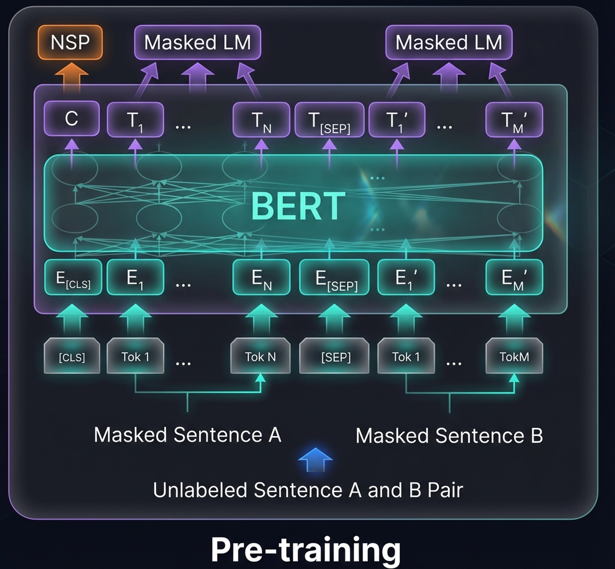
BERT’s pre-training paradigm — Masked Language Model (MLM) and Next Sentence Prediction (NSP). This approach — pre-train on massive data with self-supervised objectives, then fine-tune — became the exact template that Vision Transformers would adopt.

BERT proved that Transformers could be pre-trained at scale with self-supervised objectives and then fine-tuned to achieve SOTA on dozens of downstream tasks. ViT adopted the same strategy: pre-train on enormous image datasets, then fine-tune for classification, detection, or segmentation.

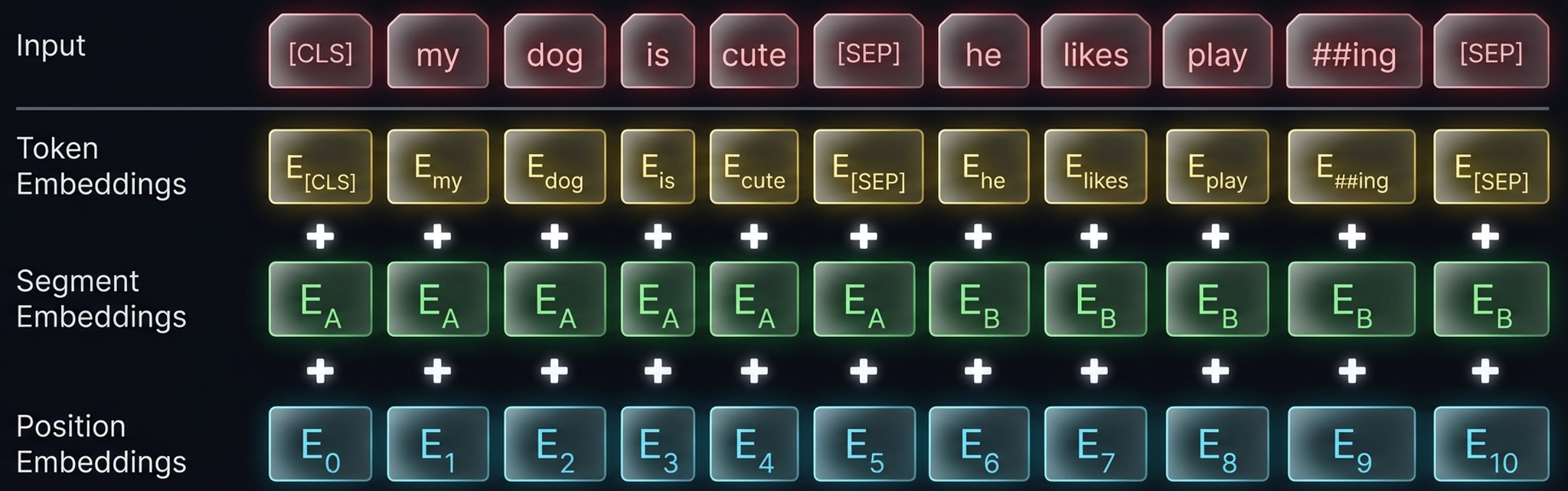
BERT’s input representation: Token Embeddings + Segment Embeddings + Position Embeddings. ViT adapts this directly — patches replace tokens, segment embeddings are dropped, and the [CLS] token is carried over for classification.

This three-component embedding scheme directly inspired ViT’s design. In ViT, image patches replace text tokens, segment embeddings are dropped (there’s only one “sentence”), and position embeddings encode where each patch sits in the image grid. The [CLS] token is carried over unchanged.

---

6. The ViT Architecture

Dosovitskiy et al. (ICLR 2021) introduced the Vision Transformer (ViT) — a pure Transformer applied to image classification with no convolutions. The paper title captures the core insight: “An Image is Worth 16×16 Words.”

Take a 224×224 image, divide it into 16×16 pixel patches (yielding 14×14 = 196 patches), flatten each patch, project it linearly, add position embeddings, prepend a [class] token, and feed the sequence into a standard Transformer Encoder. That’s it.

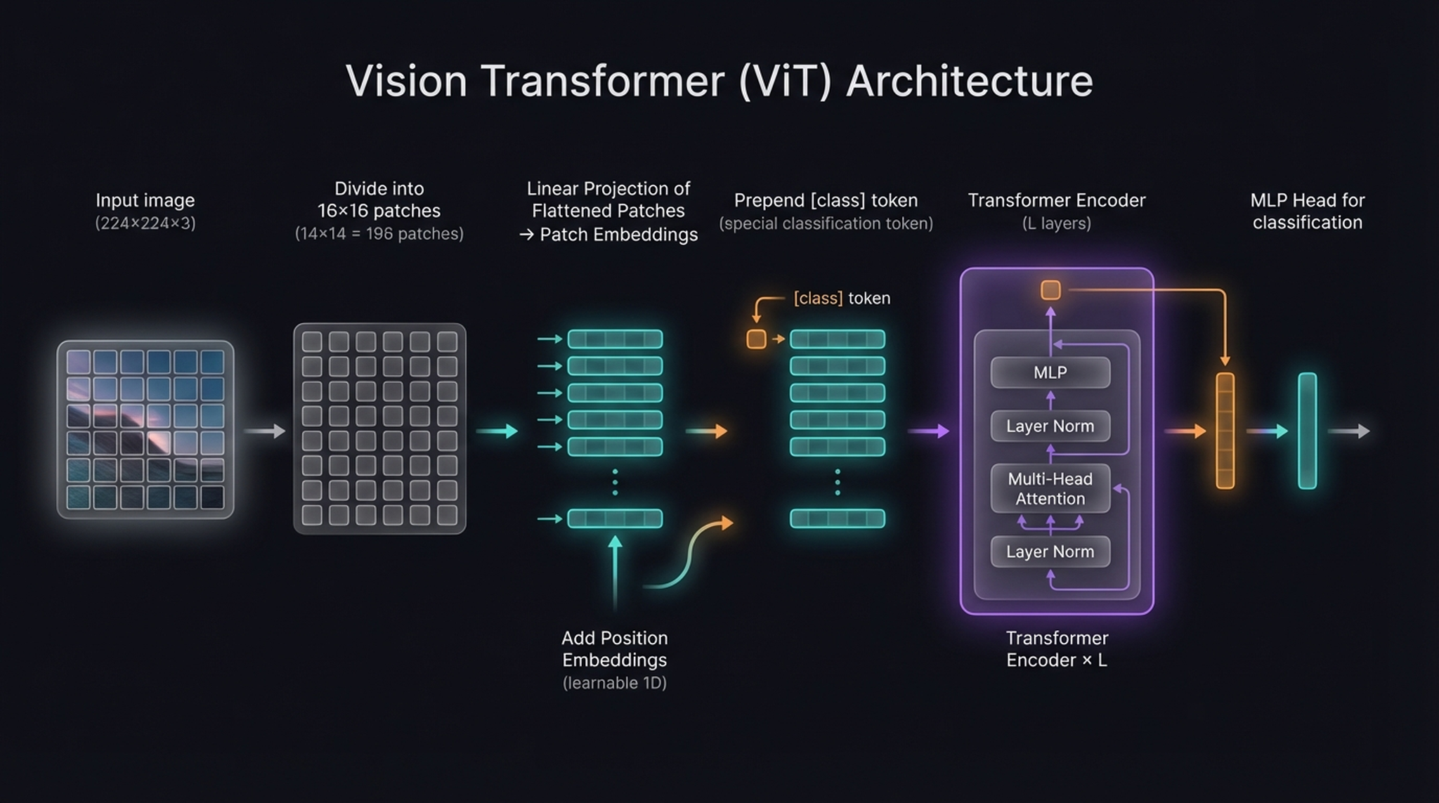
The complete ViT pipeline. An input image (224×224×3) is divided into 16×16 patches (196 total), each flattened and linearly projected. A [class] token is prepended, learnable 1D position embeddings are added, and the sequence enters a Transformer Encoder. The [class] token’s output feeds an MLP Head for classification.

The pipeline, step by step:

1. Patch Extraction. 224×224 image → 196 non-overlapping 16×16 patches, each with 16 × 16 × 3 = 768 values.
2. Linear Projection. Each 768-dim patch vector is projected to embedding dimension D through a learned linear layer (equivalent to a convolution with kernel=16, stride=16).
3. [CLS] Token. A learnable embedding is prepended at position 0.
4. Position Embeddings. Learnable 1D positional embeddings are added.
5. Transformer Encoder. L layers of (LayerNorm → Multi-Head Attention → residual → LayerNorm → MLP → residual). Note: ViT uses pre-norm — LayerNorm before each sub-layer.
6. Classification Head. The [class] token’s output → MLP → class prediction.

The critical efficiency insight: 224×224 = 50,176 pixels, but only 196 patches. Self-attention scales quadratically with sequence length, so this 256× reduction makes the computation tractable.

---

7. Wait — How Can Patches Learn Spatial Relationships?

This is the question everyone asks when they first encounter ViT: if we chop an image into isolated 16×16 patches, don’t we destroy spatial relationships? Each patch is just a tiny crop. An eye, a bit of feather, a piece of background. How can the model understand that these patches form an owl?

The answer has two parts.

First: self-attention connects all patches globally from layer 1. Unlike CNNs, where a neuron at layer l can only “see” a region proportional to l × kernel_size, every patch in ViT attends to every other patch immediately. The eye-patch doesn’t need to “know” about the beak-patch through its own 16×16 pixels. It learns about the beak through attention. At each layer, each patch’s representation is updated to reflect what all 196 patches contain and where they are.

Second: position embeddings tell each patch where it came from. Without positional information, self-attention treats the input as an unordered set. The position embeddings encode spatial location, so the model knows that patch 15 is directly below patch 1 in the image grid.

The spatial understanding doesn’t live within patches — it emerges between patches, through the interaction of attention and position embeddings.

Key insight: Patches are the tokenization, not the understanding. Self-attention is what gives ViT spatial awareness — every patch can attend to every other patch from the very first layer, which means global context is available everywhere in the network from the start.

---

8. The [CLS] Token: An Empty Vector That Learns Everything

The second question that trips people up: what is the [CLS] token?

Here’s the honest answer: it’s a randomly initialized, learnable 768-dimensional vector that contains zero image information at the input. It’s prepended to the patch sequence at position 0, and through 12 layers of self-attention, it gradually absorbs information from all 196 patches.

Think of it as a blank notepad. At layer 0, it’s empty. At each subsequent layer, the attention mechanism allows [CLS] to query all patches — “what’s in the top-left?”, “what’s in the center?”, “what are the dominant textures?” — and aggregate that information into its own representation. By layer 12, this single vector has condensed the entire image into a global representation suitable for classification.

In our Colab notebook (Experiment 3), we prove this empirically:

• At layer 0, the [CLS] embedding is nearly identical across different images (it’s the same learned parameter regardless of input).
• At layer 12, the [CLS] embedding is completely different for each image — it has absorbed the image content through attention.

Is [CLS] only for classification? No. It originated in BERT for Next Sentence Prediction. In ViT, it’s used for classification because it provides a convenient single-vector summary of the image. But for dense tasks like segmentation, you use the patch token outputs instead — each patch token carries local spatial information that the [CLS] token aggregates away. SWIN and SETR use patch tokens for exactly this purpose.

Key insight: [CLS] is an architectural trick — a dedicated aggregation token. It starts empty, fills up through attention, and provides a single-vector image summary. It’s not magic. It’s a learned parameter that becomes the image representation through 12 layers of self-attention.

---

9. Position Embeddings: 1D Labels, 2D Understanding

ViT assigns position embeddings using a flat 1D sequence: patch 1, 2, 3, …, 196. There’s no explicit encoding of rows and columns. So does the model actually learn that patch 1 is adjacent to patch 2 (horizontally) and patch 15 (vertically)?

How position embeddings work. Top: patches are flattened into Flattened Patch Embeddings. Middle: Learnable 1D Positional Encoding vectors (1 through 196). Bottom: the element-wise sum, forming the final Input to the Transformer.

Each patch embedding encodes visual content (“what”) and each position embedding encodes location (“where”). The two are added element-wise. ViT uses learnable 1D positional embeddings rather than fixed sinusoidal encodings.

This is one of the most remarkable results about ViT: give the model 1D position labels and enough data, and it will discover 2D structure on its own. Learning beats inductive bias — you don’t need to hand-code spatial information.

---

10. ViT Performance and Scaling

Let’s see the full ViT system and its performance.

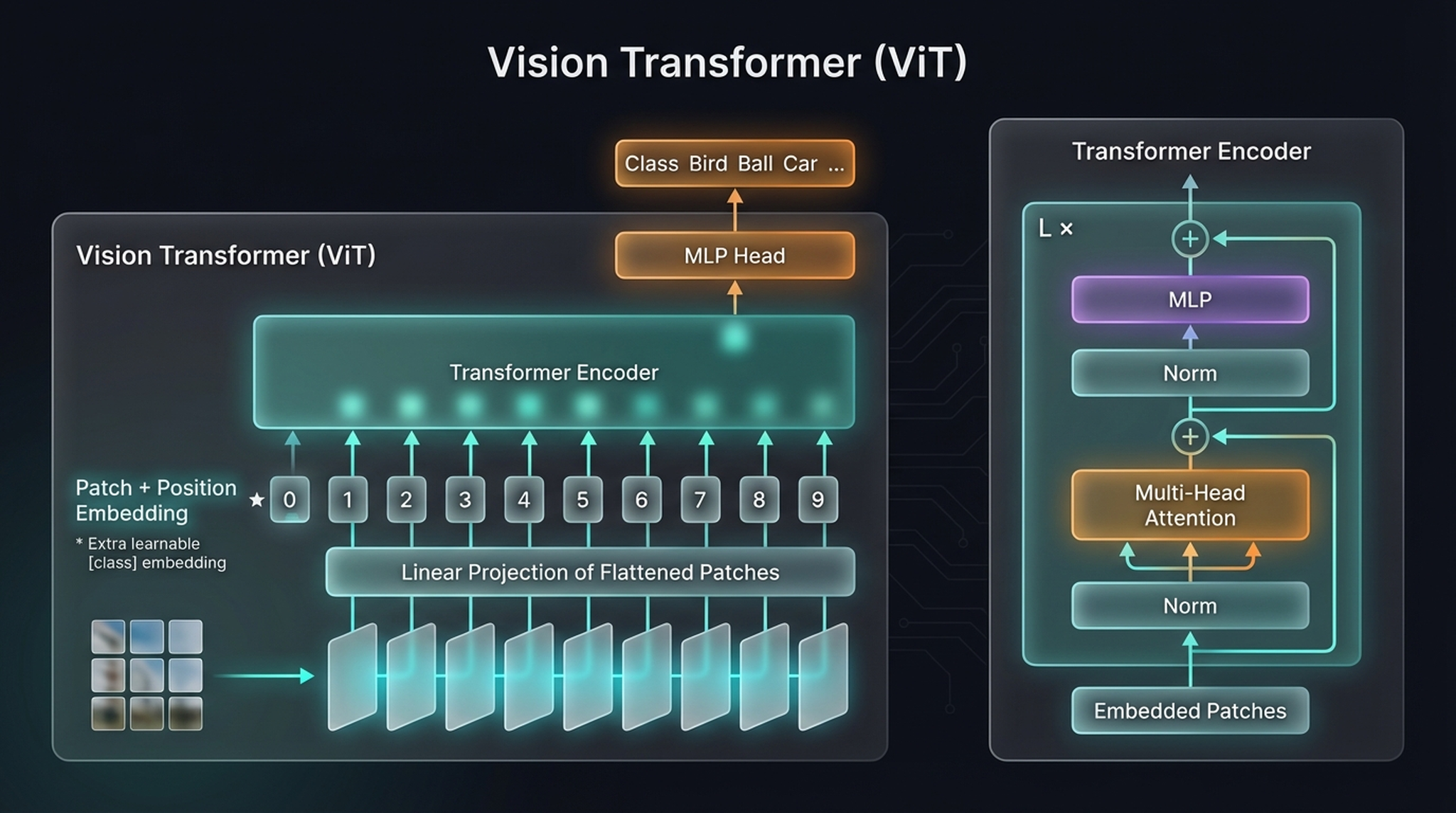
The ViT system: macro view (left) and Transformer Encoder detail (right). The [class] token (★) at position 0 aggregates information through attention. The MLP Head reads only this token’s output.

Now for the performance — and this is where things get interesting.

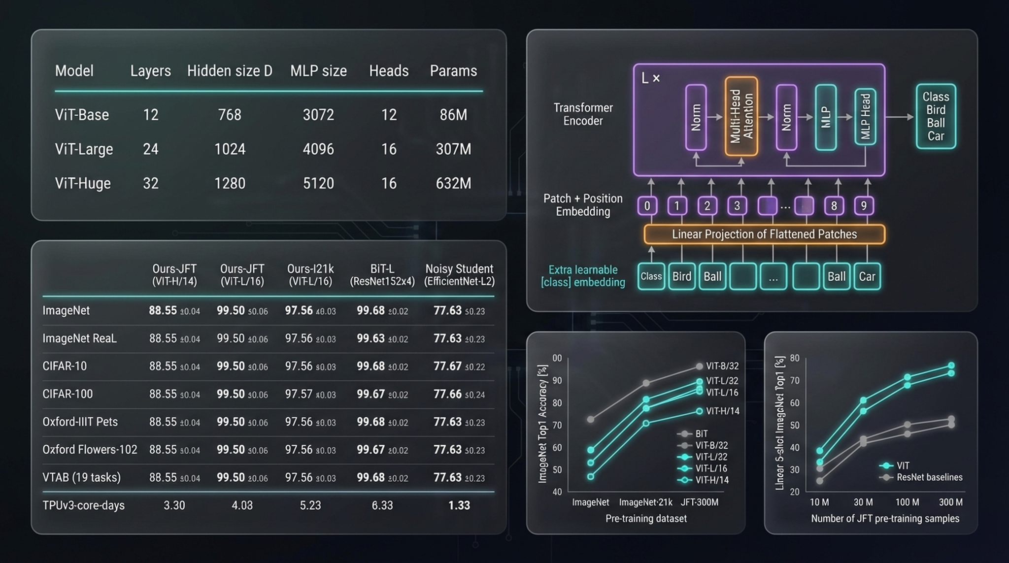
Top-left: ViT model configurations (Base: 86M params, Large: 307M, Huge: 632M). Bottom-left: benchmark accuracy. Bottom-right: scaling curves — accuracy vs. pre-training dataset size.

ViT-Huge/14 pre-trained on JFT-300M achieves 88.55% on ImageNet, surpassing BiT-L (ResNet152×4) — while requiring roughly 4× less compute to train.

But the scaling curves are the most revealing. As pre-training data grows from ImageNet (~1M) to ImageNet-21k (~14M) to JFT-300M, ViT models consistently improve while CNN baselines show diminishing returns. At small data scales, ResNets perform comparably or better. Beyond 100M samples, ViTs pull decisively ahead.

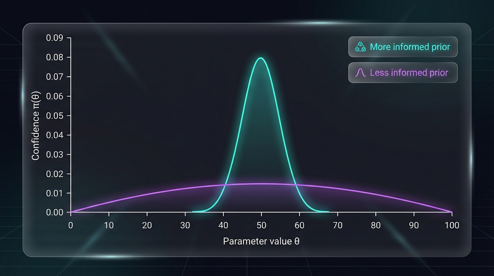
The Bayesian interpretation. Teal (narrow peak): strong priors (CNN) — high confidence in a narrow hypothesis space. Purple (broad, flat): weak priors (ViT) — lower confidence across a much wider space. With enough data, the model with weaker priors can discover solutions inaccessible to the constrained model.

This is classical Bayesian reasoning. A CNN converges quickly with limited data because its inductive biases constrain the search. But it can never discover solutions outside that narrow range. ViT, with fewer constraints, needs more data to find its footing — but with enough data, it can learn representations a CNN never could.

Key insight: The choice between ViT and CNN is a practical decision driven by your data budget. If you can pre-train at scale (or use pre-trained weights), ViTs win. If your data is severely limited, CNNs may still be better.

---

11. How ViTs See vs. How CNNs See

Do ViTs learn qualitatively different representations than CNNs? Raghu et al. (“Do Vision Transformers See Like CNNs?”, 2021) investigated this using CKA (Centered Kernel Alignment) similarity between layer representations.

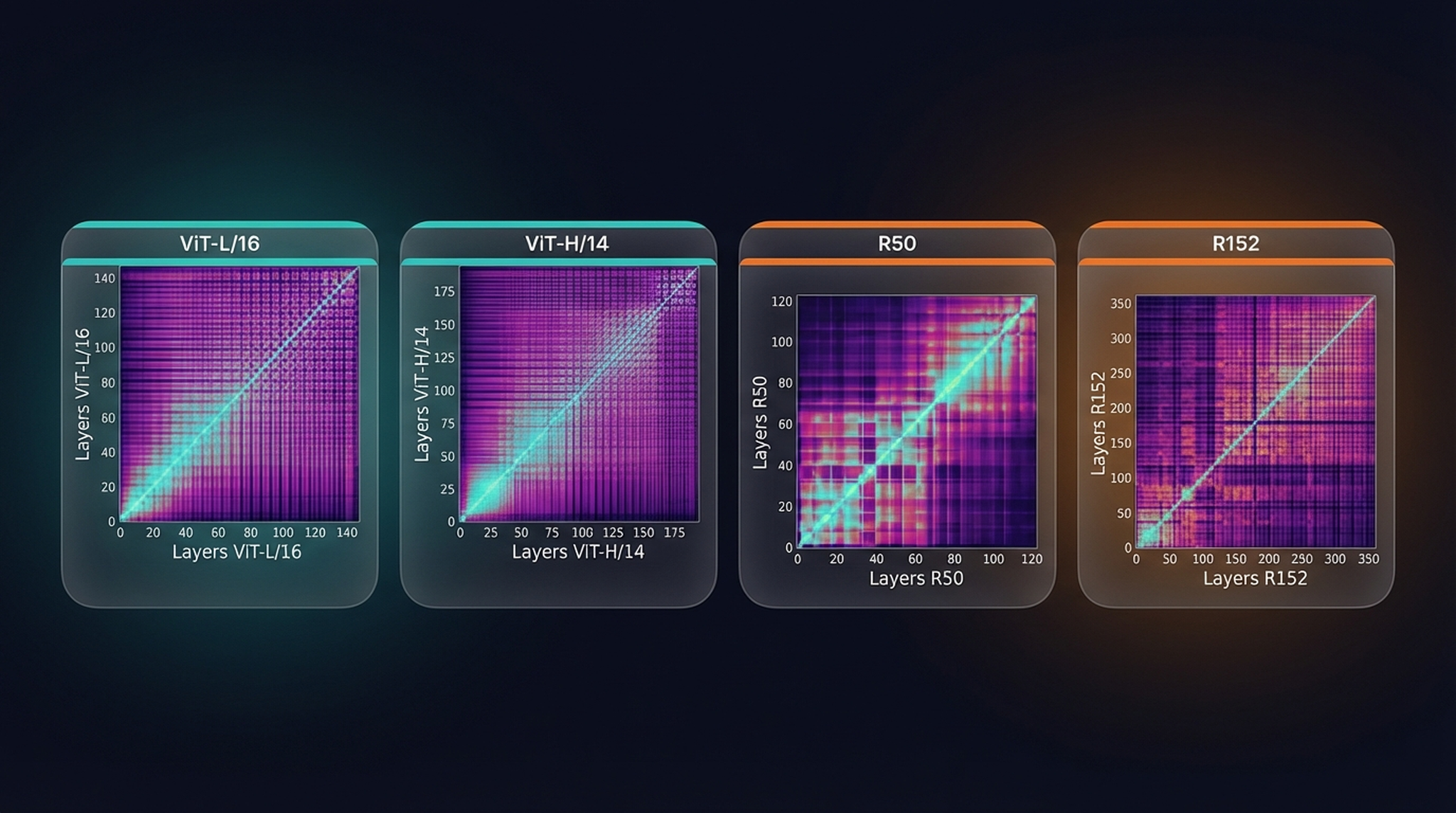
CKA similarity matrices for ViT-L/16 and ViT-H/14 (left, teal borders) vs. ResNet-50 and ResNet-152 (right, orange borders). Each axis represents a layer; brighter = more similar.

The difference is striking. The ViT plots show broad, uniform bright regions — representations across layers are relatively similar, indicating that ViTs maintain and propagate global information throughout the network. Even early ViT layers have access to long-range spatial information.

The ResNet plots show a hierarchical pattern with sharp transitions. Early layers are similar to each other, late layers are similar to each other, but there’s a clear break between them — reflecting the CNN’s progressive local-to-global feature build-up.

The reason: a CNN’s receptive field grows linearly per layer. A ViT has global receptive fields from layer 1. Every patch attends to every other patch from the start.

---

12. SWIN Transformer: Hierarchical Vision

Standard ViT processes all 196 patches at a single resolution throughout the network. Self-attention scales quadratically with token count, and ViT produces only single-scale feature maps. This limits its use for dense prediction tasks like object detection and semantic segmentation, which need multi-scale features.

Liu et al. (Microsoft Research, 2021) proposed the SWIN Transformer — “Shifted WINdow” Transformer — to address both issues.

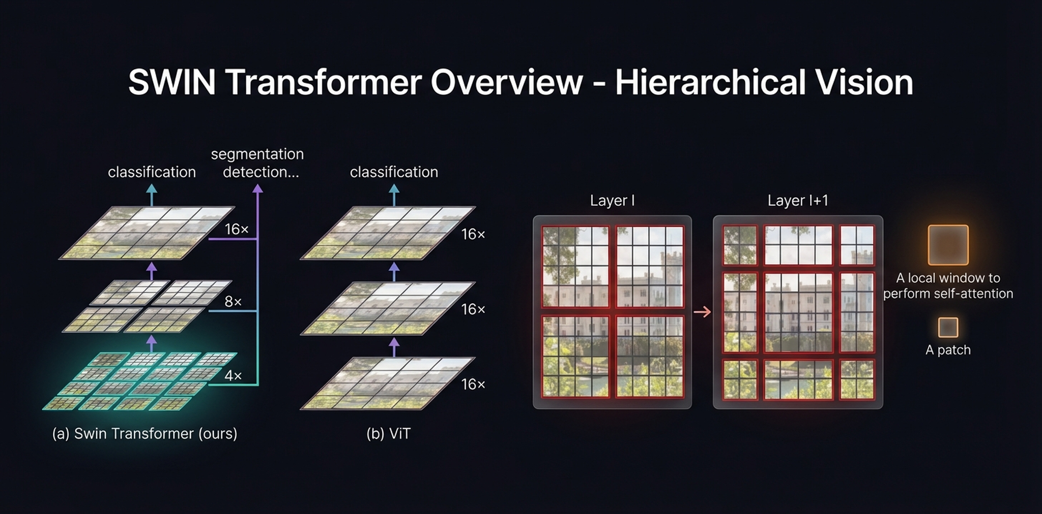
SWIN vs. ViT. Left (a): SWIN produces multi-scale feature maps at 4×, 8×, and 16× downsampling — supporting classification, detection, and segmentation. Center (b): ViT maintains fixed 16× resolution at every layer. Right: the shifted window mechanism.

The core ideas: compute attention within local windows instead of globally, and use a hierarchical structure with patch merging between stages. This gives linear complexity (vs. quadratic) and multi-scale features that plug directly into existing detection/segmentation frameworks.

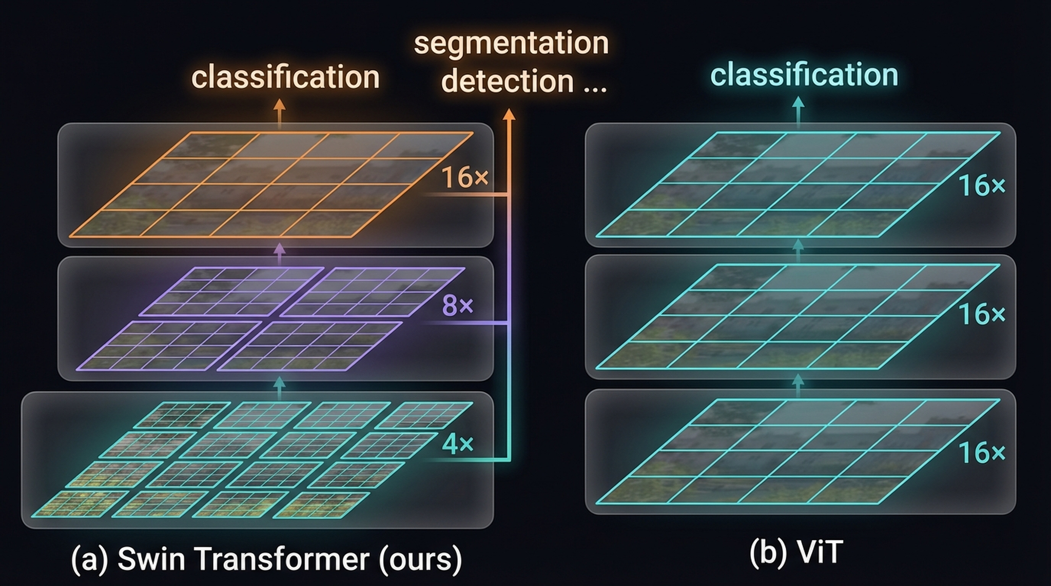
Hierarchical Feature Representation

Left (a): SWIN’s hierarchical representation — 4× (teal, many patches), 8× (purple), 16× (orange, fewer patches). Multi-scale outputs support dense prediction. Right (b): ViT’s flat 16× representation.

Patch merging layers between stages concatenate features of 2×2 neighboring patches and project linearly, halving spatial resolution while doubling channels: H/4 × W/4 × C → H/8 × W/8 × 2C → H/16 × W/16 × 4C → H/32 × W/32 × 8C. This is directly analogous to CNN pooling pyramids and can drop into FPN or UNet as a backbone.

---

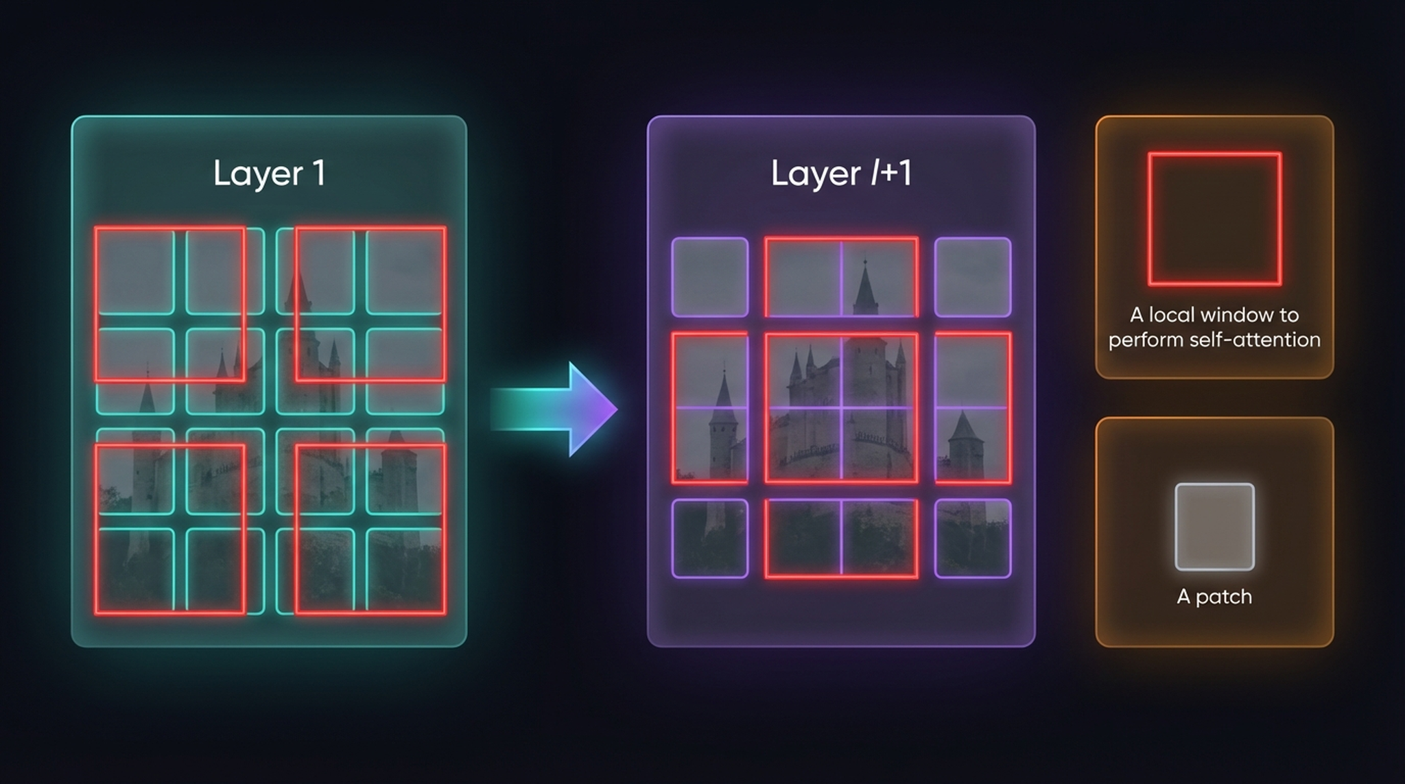
13. Shifted Windows and the Full SWIN Architecture

Computing attention within local windows is efficient, but windows are isolated from each other. The shifted window mechanism solves this.

Layer 1 (left): regular non-overlapping windows (red borders) for self-attention. Layer l+1 (right): the window grid is shifted by half a window size. New windows span previous boundaries, creating cross-window connections.

With window size M = 7, each token attends only to the 48 others in its window — much cheaper than global attention. In the next layer, shifting by (3, 3) patches means tokens at previous boundaries now share windows. Over two layers, every pair of nearby tokens has a path for information exchange.

The complete SWIN architecture. Left: four stages with progressive Patch Merging. Right: paired SWIN blocks — the first uses W-MSA (Window attention), the second uses SW-MSA (Shifted Window attention). Each block: LN → W-MSA/SW-MSA → ⊕ → LN → MLP → ⊕.

The four stages process features at increasing abstraction: Patch Partition → Stage 1 (H/4 × W/4 × C, 2 blocks) → Stage 2 (H/8 × W/8 × 2C, 2 blocks) → Stage 3 (H/16 × W/16 × 4C, 6 blocks) → Stage 4 (H/32 × W/32 × 8C, 2 blocks).

SWIN blocks always come in pairs — regular windows (W-MSA) then shifted windows (SW-MSA):

$$\hat{z}^l = \text{W-MSA}(\text{LN}(z^{l-1})) + z^{l-1}$$ $$z^l = \text{MLP}(\text{LN}(\hat{z}^l)) + \hat{z}^l$$ $$\hat{z}^{l+1} = \text{SW-MSA}(\text{LN}(z^l)) + z^l$$ $$z^{l+1} = \text{MLP}(\text{LN}(\hat{z}^{l+1})) + \hat{z}^{l+1}$$

This paired design ensures both local window attention and cross-window information flow with zero additional parameters.

---

15. Key Takeaways

Architecture	Key Innovation	Strength	Limitation
Transformer	Self-attention on sequences	Long-range deps, parallelizable	Designed for 1D sequences
ViT	Image patches as tokens	SOTA with large data, simple	O(n²) attention, single-scale
SWIN	Shifted windows + hierarchy	Linear complexity, multi-scale	More complex design

Three things to remember:

1. Patches work because of attention, not despite it. Individual patches carry minimal information, but self-attention lets them communicate globally from layer 1. Spatial understanding emerges between patches, not within them.

1. [CLS] is a learned aggregator. It starts as an empty vector and fills up with image content through 12 layers of attention. For classification, you only need this one token’s output. For dense tasks, use the patch tokens instead.

1. Training objective shapes the embedding space. Same ViT architecture trained for classification vs. contrastive learning (CLIP) produces fundamentally different representations. The architecture is a tool — what you optimize for determines what it learns.

The broader trend is clear: general-purpose architectures with minimal inductive bias, powered by large-scale data, are displacing hand-crafted domain-specific designs. The Transformer’s journey from NLP to vision — and beyond — is far from over.

---

16. Can Pure Vision Models See Wealth?

In CLIP post , we showed that CLIP can distinguish cheap from expensive bedrooms — but CLIP is multimodal. Its image encoder was shaped by 400 million image-caption pairs, absorbing human descriptions like “luxury,” “modern,” and “spacious” into its visual representations. That raises a question: how much of CLIP’s performance comes from the Vision Transformer architecture itself, and how much was gifted by language supervision?

To find out, we strip away the text entirely. We take two pure vision models — one supervised, one self-supervised — and run the same house price experiments. No text encoder. No prompts. Just raw image features.

The Models

ViT-Base (google/vit-base-patch16-224) — A standard Vision Transformer trained on ImageNet with supervised classification. It learned to distinguish 1,000 object categories: dogs, cars, birds, mushrooms. It was never trained to judge aesthetics, quality, or price.

DINOv2-Base (facebook/dinov2-base) — A Vision Transformer trained with self-supervised learning on 142 million images. No labels at all — it learned by matching augmented views of the same image. DINOv2 is widely considered the strongest pure-vision feature extractor available, producing representations that capture texture, structure, layout, and spatial relationships.

Both models produce 768-dimensional embeddings (vs. CLIP’s 512), and both use the same ViT-Base architecture. The only difference is how they were trained.

The setup is the follwoing: we embed bedroom images from the 100 cheapest and 100 most expensive houses in the dataset, then try to separate them with AI models.

Setup

import torch
import numpy as np
from PIL import Image
from transformers import AutoModel, AutoImageProcessor

# Load DINOv2 (swap model_id for ViT)
model_id = "facebook/dinov2-base"  # or "google/vit-base-patch16-224"
feature_extractor = AutoImageProcessor.from_pretrained(model_id)
model = AutoModel.from_pretrained(model_id).to(device).eval()

def embed_images(images, bs=32):
    all_emb = []
    for i in range(0, len(images), bs):
        batch = images[i:i+bs]
        inputs = feature_extractor(images=batch, return_tensors="pt").to(device)
        with torch.no_grad():
            outputs = model(**inputs)
        cls_emb = outputs.last_hidden_state[:, 0, :]  # [CLS] token
        cls_emb = cls_emb / cls_emb.norm(dim=-1, keepdim=True)
        all_emb.append(cls_emb.cpu().numpy())
    return np.vstack(all_emb)

The key difference from CLIP: we use outputs.last_hidden_state[:, 0, :] to extract the [CLS] token embedding directly from the ViT encoder. There’s no projection head, no contrastive loss against text — just the raw representation the model built from pixels alone.

---

17. Experiment 6: Centroid Separation

We apply the same centroid method: compute the mean embedding of cheap and expensive bedrooms from training data, define the “luxury axis” as the unit vector between them, and project held-out test images onto this axis.

# Split: 80 train, 20 test per group
cheap_train, cheap_test = cheap_img_emb[:80], cheap_img_emb[80:]
exp_train, exp_test = exp_img_emb[:80], exp_img_emb[80:]

# Compute centroids from training data
centroid_cheap = cheap_train.mean(axis=0)
centroid_exp = exp_train.mean(axis=0)

# Define the luxury axis
luxury_axis = centroid_exp - centroid_cheap
luxury_axis /= np.linalg.norm(luxury_axis)

# Project test images onto this axis
cheap_proj = cheap_test @ luxury_axis
exp_proj = exp_test @ luxury_axis

ViT (ImageNet):

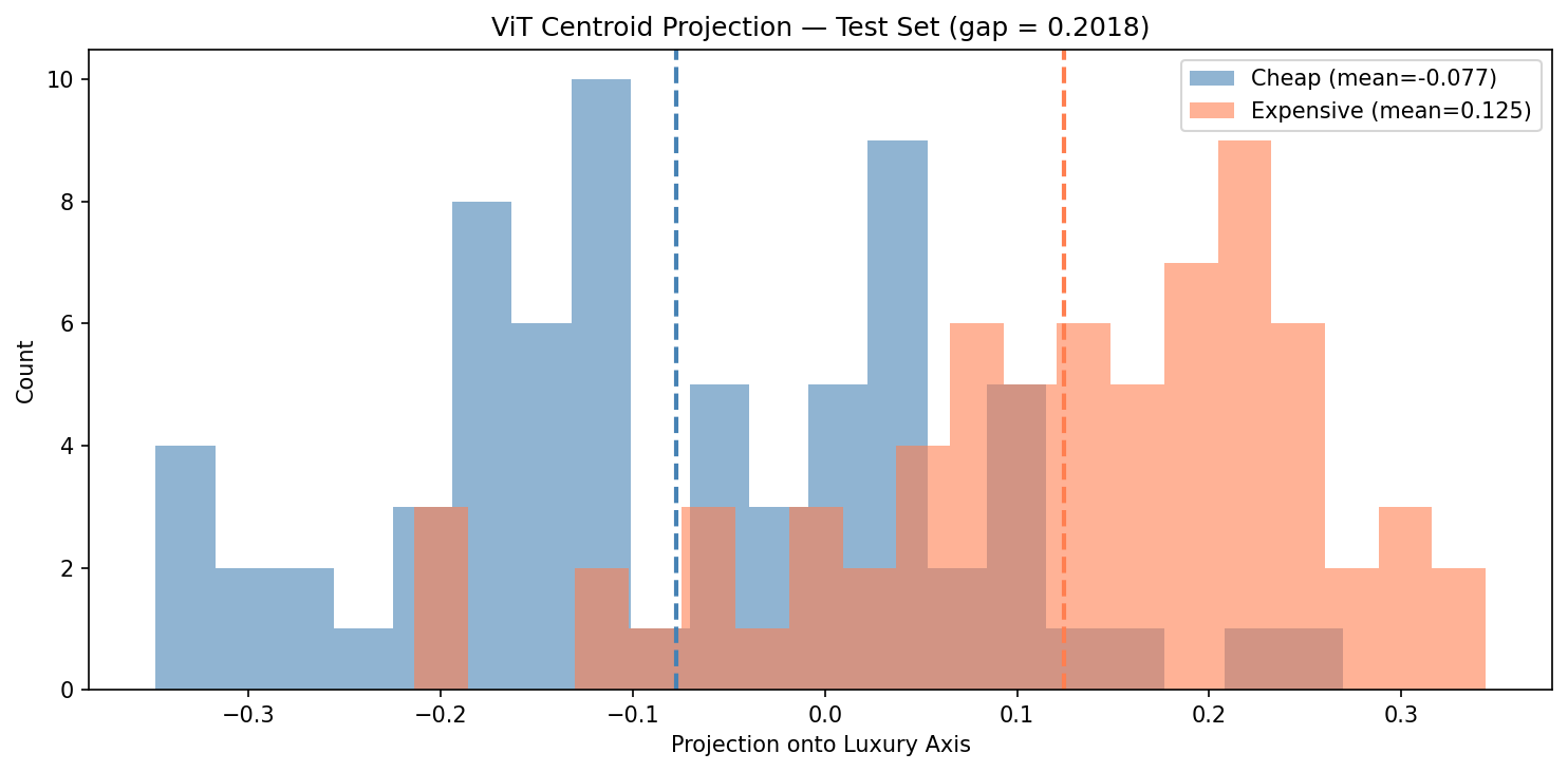
ViT centroid projection on held-out test images. Gap = 0.20. The distributions separate, but with significant overlap in the middle.

DINOv2:

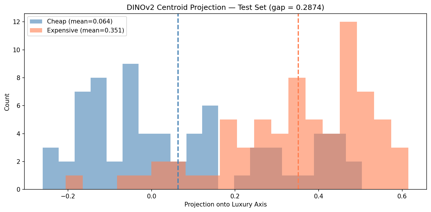
DINOv2 centroid projection on the same test split. Gap = 0.29 — nearly 50% wider than ViT, with much less overlap.

DINOv2’s centroid gap (0.29) is substantially larger than ViT’s (0.20), and comparable to CLIP’s (~0.25). The histograms tell the story visually: DINOv2 pushes the two distributions further apart, with fewer ambiguous cases in the overlap zone.

ViT-ImageNet, by contrast, learned to classify objects. It knows “this is a bed” and “this is a lamp” but spent no training signal on how beds and lamps relate to each other spatially, or whether the materials look premium.

---

18. Experiment 7: SVM vs Centroid Across Dimensions

We scale up to 150 cheapest + 150 most expensive bedrooms and compare the centroid classifier against a linear SVM across PCA dimensions:

from sklearn.svm import SVC
from sklearn.decomposition import PCA
from sklearn.model_selection import cross_val_score, StratifiedKFold

class CentroidClassifier(BaseEstimator, ClassifierMixin):
    def fit(self, X, y):
        self.classes_ = np.unique(y)
        self.centroids_ = {c: X[y == c].mean(axis=0) for c in self.classes_}
        self.axis_ = self.centroids_[1] - self.centroids_[0]
        self.axis_ /= np.linalg.norm(self.axis_)
        projs = X @ self.axis_
        self.threshold_ = (projs[y == 0].mean() + projs[y == 1].mean()) / 2
        return self

    def predict(self, X):
        return (X @ self.axis_ >= self.threshold_).astype(int)

X = np.vstack([cheap_img_emb, exp_img_emb])
y = np.array([0]*len(cheap_img_emb) + [1]*len(exp_img_emb))
cv = StratifiedKFold(n_splits=5, shuffle=True, random_state=42)

dims = [2, 5, 10, 20, 50, 100, 200, 384, 768]
for d in dims:
    X_pca = PCA(n_components=d).fit_transform(X)
    sc_c = cross_val_score(CentroidClassifier(), X_pca, y, cv=cv, scoring="accuracy")
    sc_s = cross_val_score(SVC(kernel="linear", C=1.0), X_pca, y, cv=cv, scoring="accuracy")
    print(f"PCA({d:3d}): Centroid={sc_c.mean():.1%}  SVM={sc_s.mean():.1%}")

ViT (ImageNet):

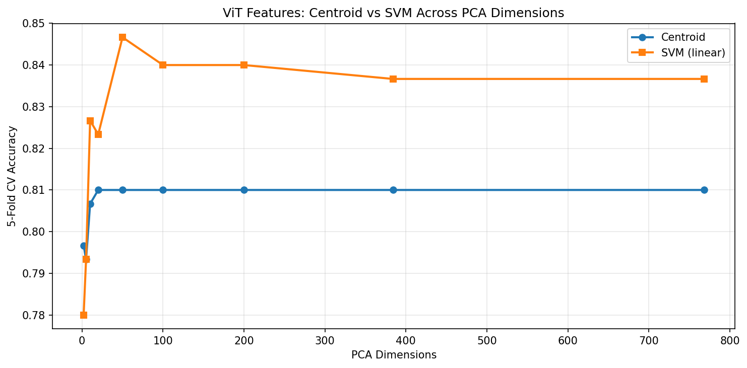
ViT features: SVM peaks at ~84.7% around PCA-50 and plateaus. Centroid saturates at ~81% and stays flat regardless of dimensionality.

DINOv2:

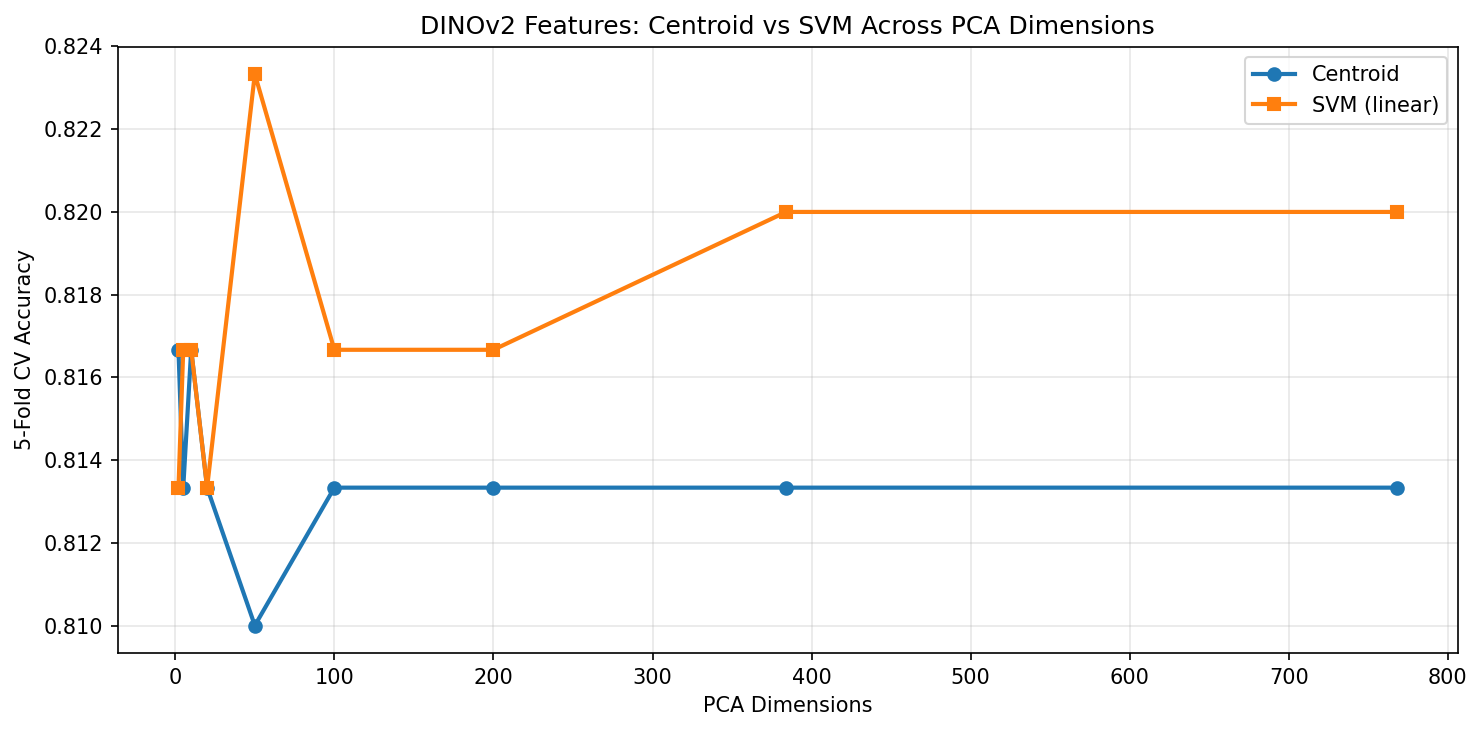
DINOv2 features: SVM peaks at ~82.3% around PCA-50. Centroid holds steady at ~81.3%. The gap between the two methods is much smaller than with ViT.

There’s an interesting reversal here. ViT’s SVM reaches a higher peak accuracy (~84.7%) than DINOv2’s SVM (~82.3%), despite DINOv2 having better centroid separation. What’s happening?

The centroid method measures only the direction between class means — it’s blind to the shape of the distributions. The SVM optimizes the full decision boundary. ViT’s ImageNet features, while less separable on average, contain discriminative information that a linear SVM can exploit in higher dimensions. This likely reflects ViT’s supervised training: it learned to create features that are linearly separable for classification, even if the class centroids aren’t maximally separated.

DINOv2’s centroid and SVM accuracies nearly converge — the centroid direction is already close to optimal. This is a signature of well-structured, symmetric representations: when the data is cleanly organized, a simple mean-based direction is almost as good as an optimized hyperplane.

The 2D decision boundaries make this contrast vivid:

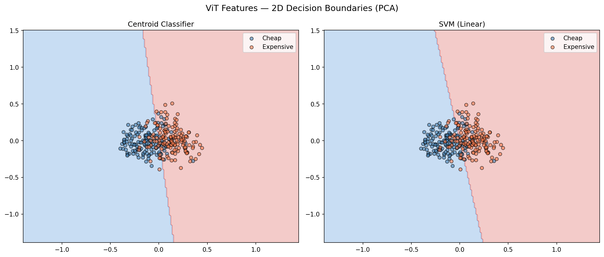
ViT in 2D: the classes overlap heavily. The data forms one mixed blob — hard for either method.

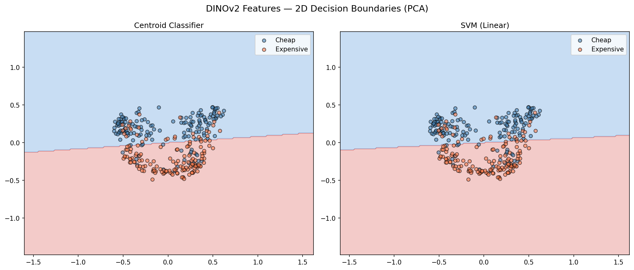
DINOv2 in 2D: the classes form two distinct clusters with a near-horizontal boundary. Much cleaner spatial structure — the model naturally separates expensive bedrooms from cheap ones in the first two principal components.

DINOv2’s 2D projection shows something ViT’s doesn’t: genuine spatial structure. The cheap and expensive bedrooms form two visually distinct clusters, separated primarily along the second principal component. In ViT’s projection, they’re mixed into a single blob. This confirms that DINOv2’s representations encode price-correlated visual features in a more organized, lower-dimensional subspace.

---

19. Experiment 8: How Much Data Do You Need?

The practical question: if you only have a handful of labeled bedroom images, which model and method should you pick?

fractions = [0.1, 0.2, 0.4, 0.6, 0.8, 1.0]
n_repeats = 10
total = len(X)

for frac in fractions:
    n_use = max(int(total * frac), 10)
    c_accs, s_accs = [], []
    for seed in range(n_repeats):
        rng = np.random.RandomState(seed)
        idx = rng.permutation(total)[:n_use]
        X_sub_pca, X_sub_full = X_pca[idx], X[idx]
        y_sub = y[idx]
        cv = StratifiedKFold(n_splits=min(5, min(np.bincount(y_sub))),
                             shuffle=True, random_state=seed)
        sc_c = cross_val_score(CentroidClassifier(), X_sub_pca, y_sub, cv=cv)
        sc_s = cross_val_score(SVC(kernel="linear", C=1.0), X_sub_full, y_sub, cv=cv)
        c_accs.append(sc_c.mean())
        s_accs.append(sc_s.mean())
    print(f"{frac*100:5.0f}% ({n_use:3d}): Centroid={np.mean(c_accs):.1%}  SVM={np.mean(s_accs):.1%}")

ViT (ImageNet):

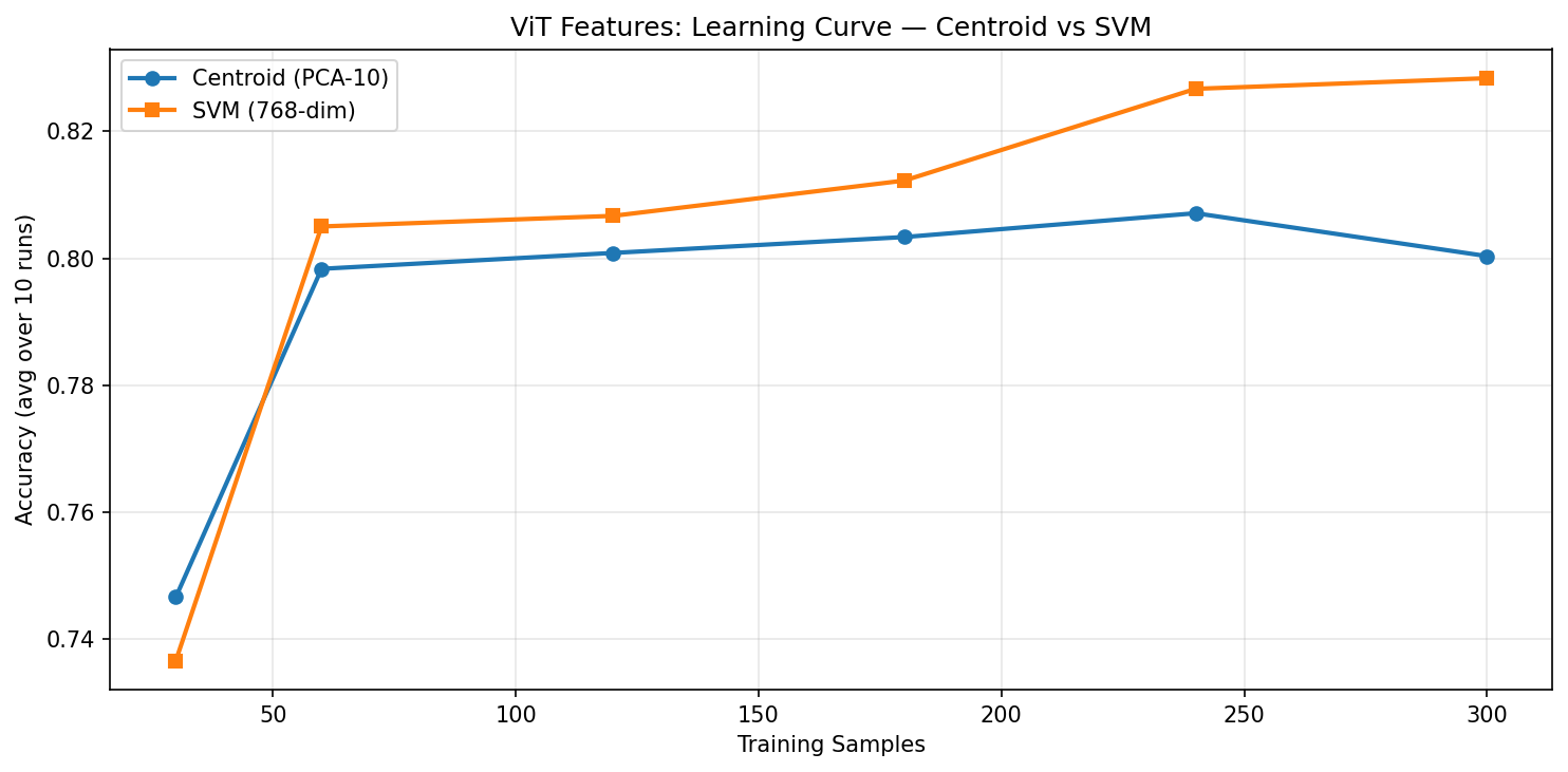
ViT learning curve: both methods start around 74–75% at 30 samples. SVM overtakes early and reaches ~82.5% at full data.

DINOv2:

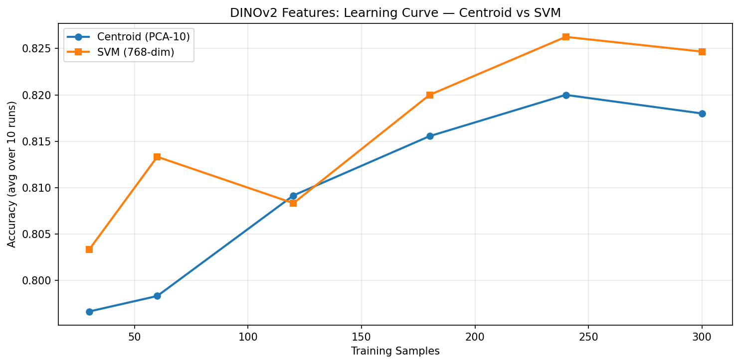
DINOv2 learning curve: both methods start higher (~80%) at 30 samples. SVM edges ahead with more data, reaching ~82.5%.

The most striking difference is the starting point. At just 30 labeled samples (~15 per class), DINOv2 already achieves ~80% accuracy with either method, while ViT starts at ~74%. That’s a 6-percentage-point head start. DINOv2’s richer representations mean you need fewer examples to reach useful performance.

Both models converge to roughly the same ceiling (~82–85% for SVM) at full data. The advantage of DINOv2 is most pronounced in the low-data regime — exactly the scenario that matters most in practice, where labeled examples are expensive to collect.

---

20. What We Learned: Vision Models Compared

Model	Training	Centroid Gap	Best SVM	Best Centroid	Strength
CLIP ViT	400M image-text pairs	~0.25	~85–86%	~83–85%	Text prompts (zero-shot)
DINOv2	142M images (self-supervised)	0.29	~82.3%	~81.3%	Best low-data, cleanest structure
ViT (ImageNet)	1.2M images (supervised)	0.20	~84.7%	~81%	Highest SVM peak

Each model has a distinct personality:

CLIP’s image encoder benefits from language supervision — it absorbed aesthetic and economic concepts through captions. This gives it the unique ability to do zero-shot classification with text prompts, plus the highest overall accuracy with data-driven methods. The text training left its fingerprint on the visual features.

DINOv2 builds the most structured representations. Despite never seeing a single label or caption, it captures fine-grained visual properties — texture, material quality, spatial layout — so thoroughly that its centroid separation actually exceeds CLIP’s. It excels in the low-data regime and produces the cleanest 2D visualizations. If you have very few labeled examples, DINOv2 is your best bet.

ViT (ImageNet) learns object-discriminative features optimized for linear separability. This is why SVM performs surprisingly well on ViT features at higher PCA dimensions, even though the raw centroid separation is the weakest of the three. It’s a reminder that classification-oriented training creates features that classifiers can exploit, even if those features don’t produce clean geometric structure.

The deeper lesson: training objective shapes what a model sees. Same architecture, same image, same bedroom — but supervised classification, self-supervised matching, and contrastive text-image alignment each cause the ViT to encode fundamentally different aspects of the visual world. The architecture provides the capacity; the training signal determines what gets captured.

---

---

References:

• Vaswani et al., “Attention is All You Need,” NeurIPS 2017
• Devlin et al., “BERT: Pre-training of Deep Bidirectional Transformers,” 2019
• Dosovitskiy et al., “An Image is Worth 16×16 Words: Transformers for Image Recognition at Scale,” ICLR 2021
• Liu et al., “Swin Transformer: Hierarchical Vision Transformer using Shifted Windows,” ICCV 2021
• Raghu et al., “Do Vision Transformers See Like Convolutional Neural Networks?,” NeurIPS 2021
• Chen et al., “When Vision Transformers Outperform ResNets without Pretraining or Strong Data Augmentations,” 2021

Dataset: Houses Dataset — Ahmed & Moustafa (2016). 535 houses, 2140 images, California sale prices. Models: google/vit-base-patch16-224 and facebook/dinov2-base via HuggingFace Transformers.