#005 How to create a panorama image using OpenCV with Python

datahacker.rs OpenCV 02.12.2020 | 0

Highlights: Nowadays, we use a number of different photo editing applications. For example, in modern smartphone cameras, we have an automatic option to create high-resolution panorama images. The essence of this process is that several photos are seamlessly combined into one original image. However, have you ever wondered how does this photo editing method works? Well, you will find out soon just continue to read this post. We will show you how to create a panorama image in Python using OpenCV.

Tutorial overview:

What is a panoramic image?
How to create a panoramic image – overview?
Detecting distinctive keypoints
Matching the points between two images
Stitching two images together

1. What is a panoramic image?

Panoramic photography is a technique that combines multiple images from the same rotating camera to form a single, wide photo. It captures images with horizontally or vertically elongated fields. This process of combining multiple photos to produce a panorama is called image stitching. So, after we rotate a camera to produce a full 360 or less degree effect we will stitch those images together to get a panoramic photo.

What is image stitching?

At the beginning of the stitching process, as input, we have several images with overlapping areas. The output is a unification of these images. It is important to note that a full scene from the input image must be preserved in the process.

2. How to create a panoramic image – overview?

In the previous post, we have learned how to extract distinctive keypoints from an image using different feature detection algorithms (SIFT, SURF, ORB). Now, using the same method as the first step we need to learn how to compare these detected features from two images in order to create a panorama.

The process of creating a panoramic image consists of the following steps.

Detect keypoints and descriptors
Detect a set of matching points that is present in both images (overlapping area)
Apply the RANSAC method to improve the matching process detection
Apply perspective transformation on one image using the other image as a reference frame
Stitch images together

For better understanding we illustrated all these steps in the following graph.

Now, let’s say that we want to create a panoramic effect with the following two images.

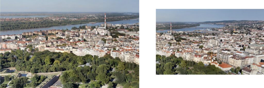
The first step in the process of creating a panorama is to align these two images. For that, we can use the detected features. Basically, we will take features in one image and match them with the features in the other image.

However, in order to accomplish our goal of creating a panorama, we need to make sure that there is a common area between these images. The reason for this is that there should be a set of distinctive keypoints detected in this overlapping region. Then, with these keypoints we have an idea of how we should stitch these images together.

Then, we need to apply perspective transformation in case that two images are not positioned on the same plane. We will use the first image as a reference frame and warp the second image so that the features in both images are perfectly aligned. This technique is called feature-based image alignment.

Once the algorithm matches identical keypoints in both images we can easily overlap them as you can see in the following image.

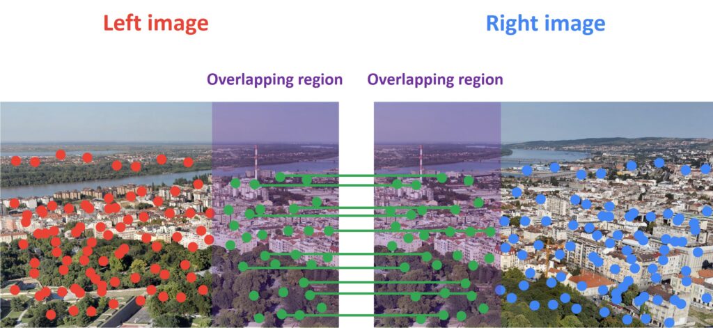
The final step is to stitch these two images together and to create a panorama image.

Now, let’s see how we can use Python and OpenCV to create a panorama image.

3. Detecting distinctive keypoints

First, let’s import the necessary libraries.

import sys
import cv2
import numpy as np

from google.colab.patches import cv2_imshowCode language: JavaScript (javascript)

To achieve more accurate results we will load our two images as a grayscale.

# Load our images
img1 = cv2.imread("first.jpg")
img2 = cv2.imread("second.jpg")

img1_gray = cv2.cvtColor(img1, cv2.COLOR_BGR2GRAY)
img2_gray = cv2.cvtColor(img2, cv2.COLOR_BGR2GRAY)

cv2_imshow(img1_gray)
cv2_imshow(img2_gray)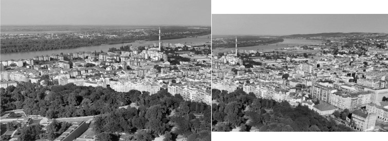Code language: PHP (php)

Now, we will use the ORB detector to extract the keypoints. First, we will create an ORB detector with the function cv2.ORB_create(). This function consists of a number of optional parameters. The most useful one is nfeatures which denotes the maximum number of features to be detected. By default, this number is set to 500 but we can change it if we want to detect more features. Next, after we specify the number of keypoints that we want to detect we will detect keypoints and descriptors in both images using the function orb.detectAndCompute().

# Create our ORB detector and detect keypoints and descriptors
orb = cv2.ORB_create(nfeatures=2000)

# Find the key points and descriptors with ORB
keypoints1, descriptors1 = orb.detectAndCompute(img1, None)
keypoints2, descriptors2 = orb.detectAndCompute(img2, None)Code language: PHP (php)

Using the function cv2.drawKeypoints we can draw key points in our image. This function consists of the following parameters: input image, detected keypoints, output image (its content depends on the value of the flag defining what is drawn in the output image), and the color of keypoints.

cv2_imshow(cv2.drawKeypoints(img1, keypoints1, None, (255, 0, 255))Code language: CSS (css)

cv2_imshow(cv2.drawKeypoints(img2, keypoints2, None, (255, 0, 255)))Code language: CSS (css)

4. Matching the points between two images

Once we have extracted the features, the next step is to match these features between our two images. Lets’ see how we can do that.

In the previous post, we learned that for each detected keypoint we have one descriptor. These descriptors are arrays of numbers that define the keypoints. So, in order to match features, we are going to compare descriptors from the first image with descriptors from the second image. We will also sort matching points by their distance in order to find the closest ones. In our code, we will use the Brute Force matcher to match the descriptors.

# Create a BFMatcher object.
# It will find all of the matching keypoints on two images
bf = cv2.BFMatcher_create(cv2.NORM_HAMMING)

# Find matching points
matches = bf.knnMatch(descriptors1, descriptors2,k=2)Code language: PHP (php)

First, we have to create the BFMatcher object using the function cv2.BFMatcher_create(). This function consists of an optional parameter normType that specifies the distance as a measurement of similarity between two descriptors. For SIFT algorithm cv2.NORM_L1 type is often used. On the other hand, for binary string based descriptors like ORB, we usually use cv.NORM_HAMMING.

The second parameter is crossCheck. By default, it is set to False. In that case, BFMatcher will find the $k $ nearest neighbors for each query descriptor. On the other hand if crossCheck==True, then the knnMatch() method will return only those matches with value $(i,j) $ such that i-th descriptor in set $A $ has j-th descriptor in set $B $ as the best match and vice-versa. In that way, the two features in both sets should match each other. Such a technique usually produces the best results with a minimal number of outliers when there are enough matches. However, in our code, this parameter is switched of because to find the best matches we will use another method.

Let’s take a closer look at one keypoint in order to see how its structure looks like. First, we can see it’s $(x, y) $ position using the .pt argument.

print(keypoints1[0].pt)Code language: CSS (css)

(427.0, 268.0)

Also, we can see its size using the .size argument

print(keypoints1[0].size)Code language: CSS (css)

31.0

Now, let’s print the descriptor of a first point.

print("Descriptor of the first keypoint: ")
print(descriptors1[0])Code language: PHP (php)

Descriptor of the first keypoint: 
[147 135 199 157  22 178 172  38 156  67  94 210 237 230 176 229 126 110  50 172 225 148  38 207 166 102 202 128  61 252 185 180]

We can also print the distance between the first keypoint in the first image and the first kaypoint in the second image.

print(matches_sorted[0].distance)Code language: CSS (css)

10.0

Now, let’s continue with our post. The next step is to define function draw_matches() that will be used to match overlapping keypoints. This function consists of the following parameters.

img1, img2 – the input images
keypoints1 – keypoints detected in the first image
keypoints2 – keypoins detected in the second image
matches – overlapping keypoins

def draw_matches(img1, keypoints1, img2, keypoints2, matches):
  r, c = img1.shape[:2]
  r1, c1 = img2.shape[:2]

  # Create a blank image with the size of the first image + second image
  output_img = np.zeros((max([r, r1]), c+c1, 3), dtype='uint8')
  output_img[:r, :c, :] = np.dstack([img1, img1, img1])
  output_img[:r1, c:c+c1, :] = np.dstack([img2, img2, img2])

  # Go over all of the matching points and extract them
  for match in matches:
    img1_idx = match.queryIdx
    img2_idx = match.trainIdx
    (x1, y1) = keypoints1[img1_idx].pt
    (x2, y2) = keypoints2[img2_idx].pt

    # Draw circles on the keypoints
    cv2.circle(output_img, (int(x1),int(y1)), 4, (0, 255, 255), 1)
    cv2.circle(output_img, (int(x2)+c,int(y2)), 4, (0, 255, 255), 1)

    # Connect the same keypoints
    cv2.line(output_img, (int(x1),int(y1)), (int(x2)+c,int(y2)), (0, 255, 255), 1)
    
  return output_imgCode language: PHP (php)

In the second line of this function, we are defining the row and the column of the first and the second image. Then, we create a black image using the function np.zeros(). This image will have the same dimensions as the output image where two input images are stitched together. That is why we will set the number of rows to the larger of the two values, and the number of columns will be the sum of both values. For a color image, we also need to create three channels and stack them together. We can do that with the function np.dstack(). This function stacks 2D arrays in a sequence along the third axis that is perpendicular to the first two axes. For instance, the height of an image is the first axis (indexed as 0), width is the second axis (indexed as 1), and RGB channels are the third axis (indexed as 2).

The next step is to create for loop which will iterate through all matches. Attribute match.queryIdx gives us the index of the descriptor in the list of train descriptors in the first image ( the index of the point in the first image we want to find a match for ). Argument match.trainIdx gives us the index of the descriptor in the list of query descriptors in the second image (the index of the matching result of that point in the second image). Then, for each item in detected matches, we extract the locations of the matching keypoints.

Next, we will draw the circles around keypoints with the function cv2.circle()and we draw the line to connect them with the function cv2.line().

Now, using the function draw_matches()we can draw matching points in the image. For better visualization, we will draw only the first 30 matches.

all_matches = []
for m, n in matches:
  all_matches.append(m)

img3 = draw_matches(img1_gray, keypoints1, img2_gray, keypoints2, all_matches[:30])
cv2_imshow(img3)

cv2_imshow(img3)

Here, we can see pairs of matching keypoints detected in both images. They are spread all over the picture. However, our goal is to extract only strong matches that are located in the overlapping region.

To keep only the strong matches we will use David Lowe’s ratio test. Lowe proposed this ratio test in order to increase the robustness of the SIFT algorithm. Our goal is to get rid of the points that are not distinct enough. Basically, we are discarding these matches where the ratio of the distances to the nearest and the second nearest neighbor is greater than a certain threshold. In this way, we will preserve only good matches.

We can do that with the following code.

# Finding the best matches
good = []
for m, n in matches:
    if m.distance < 0.6 * n.distance:
        good.append(m)Code language: PHP (php)

cv2_imshow(cv2.drawKeypoints(img1, [keypoints1[m.queryIdx] for m in good], None, (255, 0, 255)))Code language: CSS (css)

cv2_imshow(cv2.drawKeypoints(img2, [keypoints2[m.trainIdx] for m in good], None, (255, 0, 255)))Code language: CSS (css)

5. Stitching two images together

To stitch two images together we need to apply a technique called feature-based image alignment. It is the computation of 2D and 3D transformations that map features in one image to another. This technique consists of two steps. The first step is to apply RANSAC algorithm to evaluate a homography matrix. Then, we will use this matrix to calculate the warping transformation based on matched features. Now, let’s first explain what is the homography matrix?

What is a homography matrix?

In the field of computer vision, any two images of the same scene are related by a homography. It is a transformation that maps the points in one image to the corresponding points in the other image. The two images can lay on the same surface in space or they are taken by rotating the camera along its optical axis. In the chapter “Camera Calibration and Stereo Vision”, we have already covered this topic in the series of posts.

The essence of the homography is the simple $3\times3 $ matrix called the homography matrix.

$$ H=\left[\begin{array}{lll}h_{11} & h_{12} & h_{13} \\h_{21} & h_{22} & h_{23} \\h_{31} & h_{32} & h_{33}\end{array}\right] $$

We can apply this matrix to any point in the image. For example, if we take a point $A(x_{1},y_{1}) $ in the first image we can use a homography matrix to map this point $A $ to the corresponding point $B(x_{2},y_{2}) $ in the second image.

$$ s\left[\begin{array}{l}x^{\prime} \\y^{\prime} \\1\end{array}\right]=H\left[\begin{array}{l}x \\y \\1\end{array}\right]=\left[\begin{array}{lll}h_{11} & h_{12} & h_{13} \\h_{21} & h_{22} & h_{23} \\h_{31} & h_{32} & h_{33}\end{array}\right]\left[\begin{array}{l}x \\y \\1\end{array}\right] $$

Now, using this technique we can easily stitch our images together.

It is important to note that when we match feature points between two images, we only accept those matches that fall on the corresponding epipolar lines. We need these good matches to estimate the homography matrix. We detected a large number of keypoints and we need to reject some of them to retain the best ones.

Now, we need to calculate the homography. We are applying the function cv2.warpImages()which consist of parameters img1, img2, and H. The first and the second parameter are our two images and H is the homography matrix. As we already explained this $3\times3 $ matrix will be used to transform the second image to have the same perspective as the first one which will be kept as the reference frame. Then, we will extract information about the transformation of the second image and use that information to align the second image with the first one.

To find this transformation matrix, we need to extract coordinates of a minimum of 4 points in the first image and corresponding 4 points in the second image. These points are related by homography so we can apply a transformation to change the perspective of the second image using the first image as a reference frame. In the following image, you can see an example of this transformation.

Then, we will create two lists with these points. The first list called list_of_points_1 represents coordinates of a reference image, and the second list called temp_points represents coordinates of a second image that we want to transform. Then, we will apply the function cv2.perspectiveTransform()which we use to calculate the transformation matrix (homography). This function requires two arguments: a list of points in the second image and a matrix H. Finally, we can warp the second image using the function cv2.warpPerspective(). As the parameters of this function, we need to pass our second image, a transformation matrix, and the width and height of our output image.

def warpImages(img1, img2, H):

  rows1, cols1 = img1.shape[:2]
  rows2, cols2 = img2.shape[:2]

  list_of_points_1 = np.float32([[0,0], [0, rows1],[cols1, rows1], [cols1, 0]]).reshape(-1, 1, 2)
  temp_points = np.float32([[0,0], [0,rows2], [cols2,rows2], [cols2,0]]).reshape(-1,1,2)

  # When we have established a homography we need to warp perspective
  # Change field of view
  list_of_points_2 = cv2.perspectiveTransform(temp_points, H)

  list_of_points = np.concatenate((list_of_points_1,list_of_points_2), axis=0)

  [x_min, y_min] = np.int32(list_of_points.min(axis=0).ravel() - 0.5)
  [x_max, y_max] = np.int32(list_of_points.max(axis=0).ravel() + 0.5)
  
  translation_dist = [-x_min,-y_min]
  
  H_translation = np.array([[1, 0, translation_dist[0]], [0, 1, translation_dist[1]], [0, 0, 1]])

  output_img = cv2.warpPerspective(img2, H_translation.dot(H), (x_max-x_min, y_max-y_min))
  output_img[translation_dist[1]:rows1+translation_dist[1], translation_dist[0]:cols1+translation_dist[0]] = img1

  return output_imgCode language: PHP (php)

Once we have applied the function cv2.warpImages()we are ready to stitch the images. First, we are setting the condition of the minimum number of matches. In our code, that number is set to 10. That means that we need at least 10 matches to find the object. If enough matches are found, we extract the locations of matched keypoints in both the images. Then, we convert keypoints to type np.float32 because we will use them as a parameter of a function cv2.findHomography(). Now, when we have calculated our homography matrix we can finally stitch images together using the function cv2.warpImages(). It is good to remember that feature matching does not always produce 100% accurate matches. That is why cv2.findHomography() method as a parameter, uses the Random Sample Consensus (RANSAC) procedure which makes the function resistant to outliers. Using this method we can obtain accurate results even if we have a high percentage of bad matches.

# Set minimum match condition
MIN_MATCH_COUNT = 10

if len(good) > MIN_MATCH_COUNT:
    # Convert keypoints to an argument for findHomography
    src_pts = np.float32([ keypoints1[m.queryIdx].pt for m in good]).reshape(-1,1,2)
    dst_pts = np.float32([ keypoints2[m.trainIdx].pt for m in good]).reshape(-1,1,2)

    # Establish a homography
    M, _ = cv2.findHomography(src_pts, dst_pts, cv2.RANSAC,5.0)
    
    result = warpImages(img2, img1, M)

    cv2_imshow(result)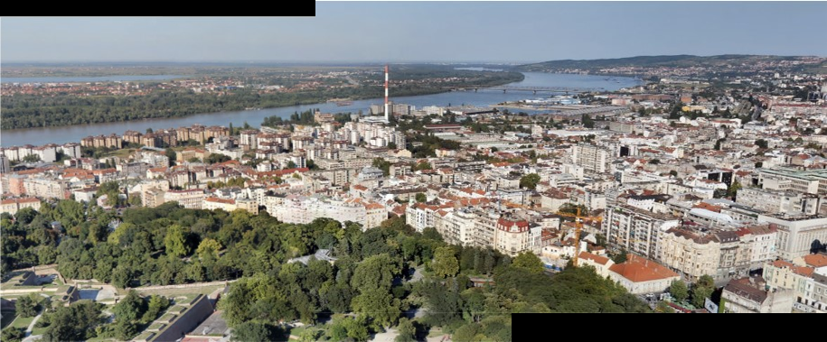Code language: PHP (php)

Summary

In this post, we have explained how to stitch two images together to create a panoramic image. In addition, we have learned how to detect and match distinctive points on an image. Furthermore, we learned to use the perspective transformation to align two images and stitch them together. In the next post, we are going to learn how we can detect contours on shapes in images.

Note that although this is a post for beginners there are too many new terms like homography RANSAC, matching features. So, to simplify this stitching method we have used only two images. Of course, this post can be much more complex if we use a series of images that are taken from different angles.

References:

[1] NOTHING AGAINST SERBIA: 5 great Panoramas of Belgrade

[2] Image Alignment (Feature Based) using OpenCV (C++/Python) by Satya Mallick

[3] Computer Vision:Algorithms and Applications by Richard Szeliski

#005 How to create a panorama image using OpenCV with Python