#026 VGGFace: Deep Face Recognition in PyTorch by Oxford VGG

Highlights: Is your goal to do face recognition in photographs or in videos? This distinguished paper, 2015, Deep Face Recognition proposed a novel solution to this. Although the period was very fruitful with contributions in the Face Recognition area, VGGFace presented novelties that enabled a large number of citations and worldwide recognition. Here, we will present a paper overview and provide a code in PyTorch to implement it.
Overview:
1. Theoretical background
This paper comes from the famous VGG group at the University of Oxford. The researchers competed with tech giants such as Google. Well, you may guess already… the previously reviewed post “FaceNet” used around 200 million face images for training across 8 million identities. It is not easy to compete with this! However, the researchers from Oxford as a first contribution presented a novelty to create a large dataset by use of automation and minimal human input.
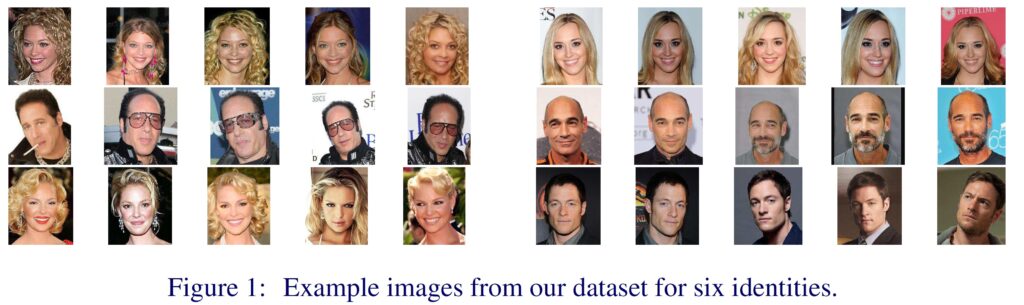
Without going into too many details, they have successfully managed to create a large dataset of celebrities. The images were found using the IMDB website and further downloaded and manually sorted. It was important for these tasks to have more face images for a single person, and the researchers managed to create 375 face images for every person. In total, they managed to gather 2,622 unique identities, thereby creating a dataset of approximately 1 million images.
Therefore, the paper had two goals.
- To create a large face database with use of a limited computing and human annotation power.
- To explore different models for the tasks of face identification and verification, including face alignment and metric learning.
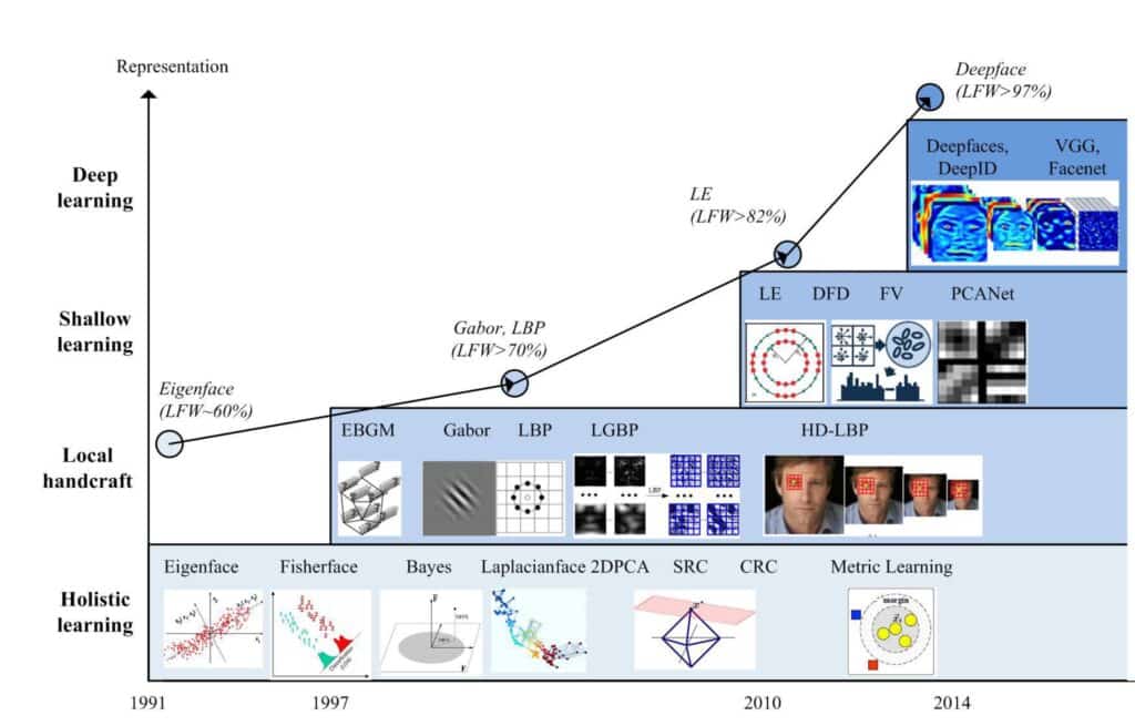
In the image below we can see the milestones in the Face Recognition area and VGGFace is included as well. [1]
2. VGGFace network architecture
This section starts with CNN descriptions used for VGGFace.
Learning a face classifier
The original problem is formulated to classify \(N=2,622 \) person identities. The authors used a deep CNN architecture denoted as a function FI to perform this N-classification problem.
The goal here was to associate each training image \(\ell_{t}, t=1, \ldots, T \), with a score vector \(\mathbf{x}_{t}=W \phi\left(\ell_{t}\right)+b \in \mathbb{R}^{N} \). In other words, the final output for every image lt, will produce the vector \(\phi (\ell_{t}) \) and this vector will be multiplied with a matrix \(W \), and a bias term \(b \) would be added. The dimension of the matrix \(W \) are \(N\times D \). That is, the final layer contains \(N \) linear predictors one per each identity. We have already explored this type of linear classifier formulation in our previous post: Linear classifiers in PyTorch: experiments and intuition. Feel free to refresh your knowledge if needed.
Next, these scores are compared to the ground-truth class identity \(c_{t} \in\{1, \ldots, N\} \) by computing the empirical softmax log-loss \(E(\phi)=-\sum_{t} \log \left(e^{\left\langle\mathbf{e}_{t}, \mathbf{x}_{t}\right\rangle} / \sum_{q=1, \ldots, N} e^{\left\langle\mathbf{e}_{q}, \mathbf{x}_{t}\right\rangle}\right) \), where \(\mathbf{x}_{t}=\phi\left(\ell_{t}\right) \in \mathbb{R}^{D} \), and \(\mathbf{e}_{c} \) denotes the one-hot vector of class \(c \).
Once the learning is complete the linear classifier can be removed. Then we will have as the output the score vectors \(\phi (\ell_{t}) \). These vectors can be further fused for face recognition and verification. For instance, we can do face verification by comparing the Euclidean distance between two vectors.
Next, these scores will be significantly improved using the triplet loss function during a network training process. Ain’t that going to be the same as FaceNet? Yeah. It is pretty similar. But, the novelty introduced with this step is to bootstrap the network as a classifier. And this pre-training process allows much faster and easier training.
Learning a face embedding using a triplet loss
The goal of triplet loss training aims to generate learning score vectors that perform well in the final application task. For instance, we can do face clustering in the Euclidean space. This is similar to the field of “metric learning”, and the further approach would strive to learn a projection that is at the same time both distinctive and compact, and also achieves a dimensionality reduction.
So, how are we gonna do that?
Well, it turns out that it is rather simple. The output \(\phi\left(\ell_{t}\right) \in \mathbb{R}^{D} \)$ that we learned in the previous section will be multiplied with a projection matrix \({W}’ \).
$$\mathbf x_{t}=W^{\prime} \phi\left(\ell_{t}\right)/ \left\|\phi\left(\ell_{t}\right) \right\|_{2}, $$
where,
$$ W^{\prime} \in \mathbb{R}^{L \times D} $$
Here, the result will be \(l^{2} \) – normalized.
Although this resembles so much the previous paragraph, there are some important differences. First of all, the output dimension is now \(L \), and not \(D \) -the number of identity classes \(L \neq D \). The \(L \) value can be set arbitrarily, and here it is initialized to 1,024. As second, the projection \({W}’ \) is used to minimize the empirical triplet loss:
$$ E\left(W^{\prime}\right)=\sum_{(a, p, n) \in T} \max \left\{0, \alpha-\left\|\mathbf{x}_{a}-\mathbf{x}_{n}\right\|_{2}^{2}+\left\|\mathbf{x}_{a}-\mathbf{x}_{p}\right\|_{2}^{2}\right\}, $$
where,
$$ \mathbf{x}_{i}=W^{\prime} \frac{\phi\left(\ell_{i}\right)}{\left\|\phi\left(\ell_{i}\right)\right\|_{2}} $$
In addition, note that we do not have a bias term in the projection as compared to the previous paragraph.
Here, \(T \) represents a learning set, whereas alpha is set to be a learning margin. Similarly, as in the FaceNet, the triplet \((a, p, n) \) is initialized with an anchor image, followed by the image of the same identity – positive, and then, the negative identity (face image of a different person).
VGGFace network architecture
Finally, in this part, we will explore the proposed network for VGGFace. You can already guess from the name what is going to be the main building block.
There are 11 blocks, and each contains an operator that is followed by one or more nonlinearities, such as ReLU activation function or max pooling. The initial layers are convolutional layers, whereas the last three layers are Fully Connected layers (FC). The complete network is shown in the table below:
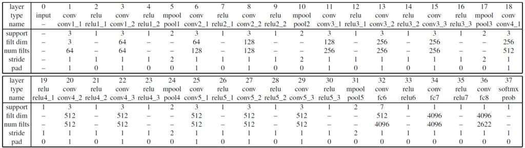
The input to this network is a face image of size \(224\times224 \) pixels. For training, an SGD algorithm is initially proposed. The network does not include batch normalization layers, and minimal data augmentation is included (flipping and random center cropping).
3. VGGFace in Pytorch
Do you know why VGG is my favorite Deep Learning network? It’s the most elegant and the simplest to implement.
So, our job here will be relatively easy. Up to now, you have probably seen the VGG network a dozen times. Here is the main class:
class VGG_16(nn.Module):
     """
     Main Class
     """


     def __init__(self):
         """
19         Constructor
         """
         super().__init__()
         self.block_size = [2, 2, 3, 3, 3]
         self.conv_1_1 = nn.Conv2d(3,   64,  3, stride=1, padding=1)
         self.conv_1_2 = nn.Conv2d(64,  64,  3, stride=1, padding=1)
         self.conv_2_1 = nn.Conv2d(64,  128, 3, stride=1, padding=1)
         self.conv_2_2 = nn.Conv2d(128, 128, 3, stride=1, padding=1)
         self.conv_3_1 = nn.Conv2d(128, 256, 3, stride=1, padding=1)
         self.conv_3_2 = nn.Conv2d(256, 256, 3, stride=1, padding=1)
         self.conv_3_3 = nn.Conv2d(256, 256, 3, stride=1, padding=1)
         self.conv_4_1 = nn.Conv2d(256, 512, 3, stride=1, padding=1)
         self.conv_4_2 = nn.Conv2d(512, 512, 3, stride=1, padding=1)
         self.conv_4_3 = nn.Conv2d(512, 512, 3, stride=1, padding=1)
         self.conv_5_1 = nn.Conv2d(512, 512, 3, stride=1, padding=1)
         self.conv_5_2 = nn.Conv2d(512, 512, 3, stride=1, padding=1)
         self.conv_5_3 = nn.Conv2d(512, 512, 3, stride=1, padding=1)
         self.fc6 = nn.Linear(512 * 7 * 7, 4096)
         self.fc7 = nn.Linear(4096, 4096)
         self.fc8 = nn.Linear(4096, 2622)
So, this definition was fairly easy. Note just one subtlety that for the layer fc6 input number of channels is hard-coded. The network shrink the original image from \(224\times224 \) onto a feature map of \(7\times7 \). Therefore, if you want to train a network on the different input image sizes make sure to adjust this number!
Now, we will have a look at the implementation of the forward method:
 def forward(self, x):
         """ Pytorch forward

         Args:
             x: input image (224x224)

         Returns: class logits

         """
         x = F.relu(self.conv_1_1(x))
         x = F.relu(self.conv_1_2(x))
         x = F.max_pool2d(x, 2, 2)
         x = F.relu(self.conv_2_1(x))
         x = F.relu(self.conv_2_2(x))
         x = F.max_pool2d(x, 2, 2)
         x = F.relu(self.conv_3_1(x))
         x = F.relu(self.conv_3_2(x))
         x = F.relu(self.conv_3_3(x))
         x = F.max_pool2d(x, 2, 2)
         x = F.relu(self.conv_4_1(x))
         x = F.relu(self.conv_4_2(x))
         x = F.relu(self.conv_4_3(x))
         x = F.max_pool2d(x, 2, 2)
         x = F.relu(self.conv_5_1(x))
         x = F.relu(self.conv_5_2(x))
         x = F.relu(self.conv_5_3(x))
         x = F.max_pool2d(x, 2, 2)
         x = x.view(x.size(0), -1)
         x = F.relu(self.fc6(x))
         x = F.dropout(x, 0.5, self.training)
         x = F.relu(self.fc7(x))
         x = F.dropout(x, 0.5, self.training)
         return self.fc8(x)
So, this was rather straight forward. Hence, you realize that coding the models itself in Deep Learning is usually not that much of an issue. However, training definitely can be challenging and requires CPU/GPU resources!
And now comes the most interesting part:
VGGNet deafeted FaceNet !!
do you believe it?
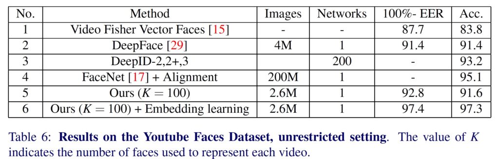
So, here is the table from the experimental results and evolutions. At the time of publishing VGGNet achieved state-of-the-art result on some datasets. But, the proposed network is of a much simpler architecture and trained on a much much smaller dataset as compared to FaceNet: 1-2 Million vs 200 Million images. Have a look at the Table below:
Anyhow, both networks as well as DeepFace were very important and achieved state-of-the-art results in 2015. Have a look at this nice pictorial representation of the Deep Learning Networks and milestone Facial Recognition models from [1].
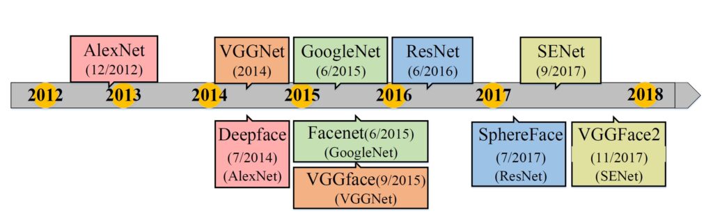 As you can see the top row reresents the typical network arhitectures used for object cllasification, and the bottom row describes the well-known face recognition algorithms that are used in typical arhitectures. The sam color rectangles are used to present the algorithms that use the same arhitecture. It is easy to see that thearhitecture.s of Deep FR have always followed those of deep object classification and evolved from AlexNet to SeNet repidly.
Summary
In this post, we have covered the popular paper “Deep Face Recognition: A Survey” written by the famous VGG group from the University of Oxford. We introduced the theoretical background of this paper, and also provided a detailed explanation of the VGG Face network architecture. Furthermore, we learned about face embedding using a triplet loss, and finally, we have learned how to build this model in Pytorch.
And that is all. We hope you enjoyed reading this post Till next time!
References
[1] https://arxiv.org/pdf/1804.06655.pdf
[2] https://github.com/prlz77/vgg-face.pytorch/blob/master/models/vgg_face.py