#004 PyTorch – Computational graph and Autograd with Pytorch

Highlights: In this post, we will introduce computation graphs – a systematic and easy way to represent our linear model. A computation graph is a fundamental concept used to better understand and calculate derivatives of gradients and cost function in the large chain of computations. Furthermore, we will conduct an experiment in Microsoft Excel where we will manually calculate gradients and derivatives of our linear model. Finally, we will show you how to calculate gradients with PyTorch using the Autograd module.
Tutorial Overview:
- Computation graph – introduction
- An example of a computation graph
- Chain rule
- How to optimize parameters in Excel
- Automatic differentiation module in PyTorch – Autograd
- PyTorch vs Excel
1. Computation graph – introduction
Let’s first explain why do we need a computation graph? To answer this question, we have to check how the computation for the linear model is organized.
In our previous post we designed s very simple linear model which takes an input \(x \) and predicts the output \(\hat{y} \).

$$ \hat{y} = xw+b $$
The parameters \(w \) (weight) and \(b \) (bias) are unknown to us. So, the main goal of our analysis was to determine the values for \(w \) and \(b \).
To do that we applied forward pass and calculated loss and cost functions.
$$ loss=(\hat{y}-y)^{2}=(xw-y)^{2} $$
$$ cost=\frac{1}{N}\sum_{n=1}^{N}loss_{n} $$
$$ cost=\frac{1}{N}\sum_{n=1}^{N}(\hat{y}_{n}-y_{n})^{2} $$
Then, we trained our linear model to calculate the global minimum of the cost function. This process requires a gradient-based optimizer. So, to optimize our model we applied a Gradient descent algorithm. In this way, we were able to find optimal values of \(w \) and \(b \).
As we already mentioned, for this example we used a very simple linear model. So the computation of the gradients was quite an easy task. We just calculated the derivative of cost with respect to \(w \) using the following equation:
$$ Gradient = \frac{dJ}{dw} $$
However, for more complex models, computation of the gradients is not such an easy task. In particular, for deep neural networks with multiple layers, it is impossible to derive the gradients for a huge number of parameters. So, the question is, how can we efficiently compute gradients in the model with a huge number of parameters? To do that we will use computation graphs.
The main idea of computation graphs is to decompose complex computations into several sequences of much simpler calculations. There are two important principles in this process:
- Forward pass or forward propagation step: takes training points \(x \) and \(y \) as input and computes the output of our linear model – a cost.
- A backward pass or backpropagation step: is used to train our linear model to calculate the global minimum of the cost function. This process requires a gradient-based optimizer and for that, we usually apply a Gradient descent algorithm.
The basic idea of this method is that both the forward pass and the backward pass is to store and reuse intermediate results instead of recomputing them. Without this decomposition, it wouldn’t be impossible to optimize complicated deep neural networks with millions of parameters.
Now let’s explain a computation graph in more detail.
2. An example of a computation graph
First, let’s take a look at the following example of the computation graph.

As you can see a computation graph has three kinds of nodes:
- input nodes painted in blue are the input points from the data set.
- parameter nodes painted in orange are nodes where the parameters of the model are stored. These parameters will be updated to compute the cost. Our goal is to calculate gradients for these parameters because this is what we want to estimate at the end of the process.
- computation nodes painted in yellow are used for computation of the output (cost function stored in the final node). We also have intermediate compute nodes where we compute the previous nodes, inputs, or parameters. For example, if we want to multiply two parameters, we can create a new variable and assign it to the result of our product.
In the image above we have the same example of linear regression as in the previous post. To compute the cost we need to take four steps. First we need to multiply the input \(x \) with parameter \(w \). So to do that we created the variable \(u \) assigned that variable to the product of \(x \) and \(w \). Then, in the second step, we just added bias \(b \) to the \(u \). In that way, we calculated \(\hat{y} \) which is the prediction of our model. In the third step in order to compute a cost we need to calculate an error which is equal to \(\hat{y}-y \) where \(y \) is the input from the data set. Again, we assigned our result to the new variable \(e \). Finally, in the fourth step, we need the square of this variable and assign that results to the variable \(\mathcal{L} \) which is the denotation for cost.
So, this is how we can decompose complex computations into a sequence of simpler computations using this graphical formulation.
$$ \frac{dJ}{dw}=\frac{1}{N}\sum_{n=1}^{N}(x^{(i)},y^{(i)}, w^{(i)}) $$
3. Chain rule
In order to understand the backpropagation pass, we need to understand one simple rule called the chain rule. It is used when we have two functions \(g \) and \(f \) where \(f \) depends on the result of a function \(g \), and function \(g \) depends on some value \(x \). Then, the derivative of the function \(f \) with respect to the parameter \(x \) is equal to the product of the derivative of the function \(f \) with respect to \(g \) and derivative of the function \(g \) with respect to \(x \).

To better understand the chain rule lets’ take a look at the following example.

Suppose that we are analyzing just one node in the big neural network. This node is connected to many other layers and eventually it will produce a cost \(J \). Here, we have the function \(z \) that takes \(x \) and \(y \) as inputs. Our goal is to calculate the gradient of cost. To do that we need to calculate partial derivative of \(J \) with respect to \(x \) – \(\frac{\partial J}{\partial x} \), and also to calculate calculate partial derivative of \(J \) with respect to \(y \) – \(\frac{\partial J}{\partial y} \). So, let’s apply the chain rule and calculate partial derivatives.
So, let’s say that \(x=2 \) and \(y=4 \). First we can apply a forward pass and calculate the output \(z =x\cdot y \).
Next, we need to apply a backpropagation in order to calculate the local gradients, \(\frac{\partial z}{\partial x} \) and \(\frac{\partial z}{\partial y} \). We can do this in the following way.

Now, let’s suppose that we already computed the partial derivative of \(J \) with respect to \(z \) – \(\frac{\partial J}{\partial z}=5 \). According to the chain rule \(\frac{\partial J}{\partial x} \) is equal to the product of the \(\frac{\partial J}{\partial z} \) and local gradient \(\frac{\partial z}{\partial x} \). Similarly, \(\frac{\partial J}{\partial y} \) is equal to the product of the \(\frac{\partial J}{\partial z} \)and local gradient $latex \frac{\partial z}{\partial y}.

Here we constructed a very simple example so that you can better understand the idea behind the chain rule. Notice that in this case, both the input and the output values are scalars.
$$ x\in \mathbb{R} $$
$$ y\in \mathbb{R} $$
$$ \frac{\partial y}{\partial x}\in R $$
So, given the scalar input and scalar output, the derivative of the output with respect to input tells us the local linear approximation. In other words, if the input \(x \) changes by a small amount how much will \(y \) change.
However, in practice, we usually work with vector value functions. If that is the case, we will often apply the type of derivative that is used when the function has a vector as an input and produces a scalar as an output. This type of derivative is called gradient and it is actually a vector of the same size as an input. So, each element of this gradient vector will tell us how much output will change if the corresponding element of the input vector changes by the small value.
$$x\in R^{N} $$
$$ y\in \mathbb{R} $$
$$ \frac{\partial y}{\partial x}\in R^{N} $$
$$ \left ( \frac{\partial y}{\partial x} \right ){n}=\frac{\partial y}{\partial x_{n}} $$
Now, let’s see how we can apply chain rule to our linear model.
Applying chain rule to the linear regression model
First, we will apply a forward propagation step in order to calculate the loss of a single point from our data set. Remember that loss \(\mathcal{L} \) is the squared error of a single point, and a cost is the average of all losses. So, we will calculate the loss of a single point \((x,y) \) where \(x=1 \) and \(y=2 \). In order to do that, we also need to guess initial values for parameters \(w \) and \(b \). So, lets say that \(w=5 \), and \(b=1 \). Now, we can easily compute a loss as it is shown in the following computation graph.

Now, after running this forward pass in the direction of green arrows, where we have calculated the value of \(\mathcal{L} \), we are going to run a backward pass in the opposite direction. So, we will start from the output \(\mathcal{L} \), and then we will backpropagate gradients from the output node to each individual node. In this way, at each individual node, we will be able to read off the gradients with respect to \(\mathcal{L} \) and the variable in that particular node. In the following illustration, you can see how the backpropagation step looks like. Here, we are using two different colors to separate two different types of quantities. For backpropagated gradients, we are using red color for local gradients we are using a blue color.

As you can see in the image above, backward pass first computes the gradient of \(\mathcal{L} \) with respect to itself. So we will calculate the partial derivative of \(\mathcal{L} \) with respect to \(\mathcal{L} \) which is obviously equal to 1.
Now, we need to calculate the gradient of \(\mathcal{L} \) with respect to value in the next node which is an error \(e \). According to the chain rule we will multiply \(\frac{\partial \mathcal{L}}{\partial \mathcal{L}} \) that we already calculated and a local gradient \(\frac{\partial \mathcal{L}}{\partial e} \). Note that in this step, the local gradient is always equal to the back-propagated gradient.
Now, we can do one step further where we want to calculate the gradient of a \(\mathcal{L} \) with respect to our prediction \(\hat{y} \). Again we can apply the chain rule which states that \(\frac{\partial \mathcal{L}}{\partial \hat{y}} \) is equal to the previous back-propagated gradient multiplied with the local gradient:
$$ \frac{\partial \mathcal{L}}{\partial \hat{y}}= \frac{\partial \mathcal{L}}{\partial e} \frac{\partial e}{\partial \hat{y}} $$
So, in the same manner, we can continue to calculate local gradients and apply the chain rule for every node in the computation graph. Finally, we will be able to compute the gradients of \(\mathcal{L} \) with respect to parameter \(w \). Note, that we did not compute the derivative of the variable \(u \) in our example. We don’t need to do that because \(x \) is a constant and the derivative of a constant is equal to 0.
So, that is how we are going to calculate \(\frac{\partial \mathcal{L}}{\partial \hat{w}} \). However, our loss is dependent on both \(w \) and \(b \). So, we also need to calculate gradient of \(\mathcal{L} \) with respect to parameter \(b \). Therefore we will also chose a random value for \(b \) and compute \(\frac{\partial \mathcal{L}}{\partial b} \) in the same way like we calculated \(\frac{\partial \mathcal{L}}{\partial w} \) in the previous example.
4. How to optimize parameters in Excel
Now let’s see how we are going to apply a chain rule to multiple data points from our data set. We will calculate it by hand in Microsoft Excel order to show you how this is done step by step. Yes, that is right. We will use Excel to optimize our parameters.
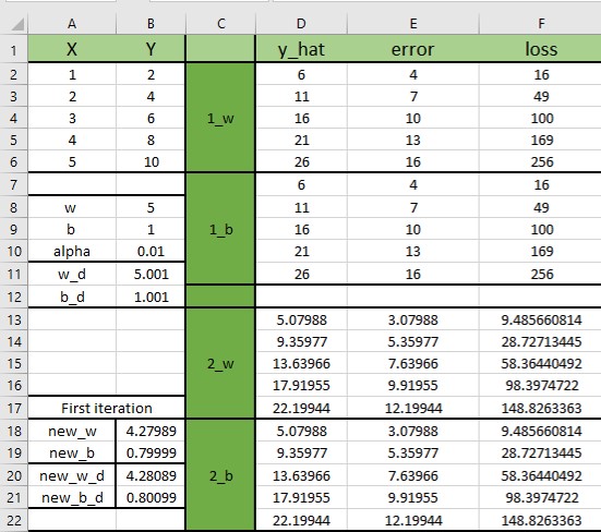
Here in the columns \(A \) and \(B \) we have values of our data points. We can see that when \(x \) is equal to 1, \(y \) is equal to 2. Again we will use the same simple regression model where \(y=wx \)
From this equation, we can already conclude that our data are composed in such a way that \(w=2 \). However, we still don’t know the value of \(w \). Remember, our goal is to optimize parameters \(w \) and \(b \) in such a way that our cost function is minimized.
We will start with some random values for both parameters: \(w=5 \) and \(b=1 \). Once again we applied forward propagation and calculated \(\hat{y} \), error, and loss. Then, we will perform the following trick. We will calculate the partial derivative of a loss with respect to \(w \) in such a way that we nudge our parameter \(w \) for one small value. So, our updated value of \(w \) will become equal to 5.001. We can say that this is indeed a small change. However, this small change will result in updating the values of y_hat, error, and loss as you can see in the following example.
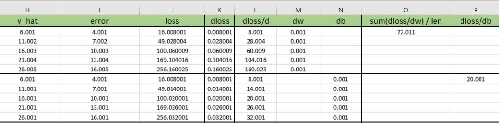
Then, we will calculate the difference between updated values and our initial values. So, when we calculate the updated loss for \(w= 5.001\) we can see that it is increased by 0.008. Then, we can calculate our gradient in the following way:
Initial values of \(w \) and \(\mathcal{L} \):
$$ w = 5 $$
$$ \mathcal{L} = 16 $$
Updated values of \(w \) and \(\mathcal{L} \):
$$ w_{u}= 5.001 $$
$$ \mathcal{L}_{u}= 16.008001 $$
$$ \frac{16.008001 – 16 }{5.001 – 5} = \frac{0.008001 }{0.001} = 8.001 $$
$$ \frac{\mathrm{d}\mathcal{L} }{\mathrm{d} w} = 8.001 $$
As you can see we obtained our gradient which is equal to 8.001. We know that this is correct because in the previous example we obtained the same result. This value tells us how fast our gradient is changing for this particular data point. So, when the gradient is higher it seems that we will be further away from the local minima that we are searching for.
Next, we will repeat this calculation for all five data points. Therefore, we will actually obtain five values for our gradient. You can see that all these values are positive. That means, according to the gradient descent algorithm that we should decrease the value of \(w \) in the next epoch.
To calculate our decreased value of \(w \) we will use the following formula:
$$ w: = w-\alpha \cdot \frac{d\mathcal{L}}{dw} $$
where \(\alpha \) is learning rate. In our case \(\alpha=0.01 \). So, now when we know all values we can calculate our updated value of \(w \).
$$ w: = 5-0.01 \cdot 72.011 $$
$$ w:=4.27989 $$
Here, \(\frac{d\mathcal{L}}{dw} \) is an average of all loss derivatives with respect to five data points. Note that once we calculate the value of \(w \), we will calculate the value for \(b \) using the same method. We will nudge \(b \) for 0.001 while keeping our initial value of \(w=5 \). The updated value of \(b \) will be calculated with the following formula:
$$ b: = b-\alpha \cdot \frac{d\mathcal{L}}{db} $$
Now, we will enter the second iteration. Here, the initial values of \(w \) and \(b \) will be our updated values that we calculated in the previous step. We will nudge \(w \) and \(b \) for the value of 0.001 and repeat the same process. Then, we will continue to update values for \(w \) and \(b \) until the difference between the updated value and the previously calculated value of \(w \) and \(b \) is a really small number. Once we reach that point we will know that we optimized our parameters successfully.
So, now we’ve learned how to optimize the parameters of our linear model. Next, we will see how we can implement this knowledge in PyTorch.
5. Automatic differentiation module in PyTorch – Autograd
To calculate gradients and optimize our parameters we will use an Automatic differentiation module in PyTorch – Autograd. The Autograd system is designed, particularly for the purpose of gradient calculations.
Before we start, first let’s import the necessary libraries.
import numpy as np
import matplotlib.pyplot as plt
import torch
Now, let’s have a look at a simple example of how we can calculate the gradients or derivatives. Let’ say that we have a simple equation:
$$ y=3x^{2}+4x+2 $$
Here, \(x \) is an independent variable, while \(y \) is a dependent variable. In the following image we can see the computational graph of this equation.

If \(x=3 \) we can apply the forward pass and calculate the value of \(y=41 \). Then, we can apply a backward pass and calculate the derivative of \(y \) with respect to \(x \). As you can see in the image above we obtained the result for \(\frac{dy}{dx}=22 \)
Now, let’s see how we can calculate this equation in Python with PyTorch. First, we will define \(x \) as a tensor with function torch.tensor() and we will set the requires_grad parameter to be True. This will automatically compute the gradients for us.
x = torch.tensor(3., requires_grad=True)Then, we define the function \(y \). After writing down our equation we will get that \(y \) is equal to 41.
y = 3*x**2 + 4*x + 2
print(y)
tensor(41., grad_fn=<AddBackward0>)Now, we want to calculate the derivative of \(y \) with respect to \(x \). For that, we will use a neat function .backward() on the variable \(y \). Our result will be stored in x.grad variable. So, we will just print x.grad and will get the value of 22 which is correct.
y.backward()
print(x.grad)tensor(22.)How to turn off the gradient calculations?
Now, you may be wondering, can we turn the gradient calculations off? Let’s have a look at the following example.
x = torch.tensor(3., requires_grad=True)
print(x)
tensor(3., requires_grad=True)If we set the requires_grad parameter to be True, and print the \(x \) variable, it will be stored as a tensor that has a certain value (in this example \(x=3 \)), and a parameter requires_grad=True. Now, what if we want to turn this \(x \) to be a constant without the gradients? There are several ways to do that, but we will explain the two most commonly used methods.
The first method is very simple. We just need to set the \(x \) to be equal to x.requires_grad_(false). If we print \(x \), we can see that it is just a tensor with a scalar value of 3.
x = x.requires_grad_(False)
print(x)tensor(3.)Another way to convert \(x \) to a constant is to apply the function x.detach() which will turn the gradient calculation off.
x = x.detach()
print(x)tensor(3.)Gradient accumulation effect
One very useful function in Python is the grad.zero_() function. One interesting thing about PyTorch is that when we optimize some parameters using the gradient, that gradient is still stored and not reset. Then, when we calculate the gradient the second time, the previously calculated gradient and the newly calculated gradient will add up. The best way to understand this is by looking at an example.
x = torch.tensor(3., requires_grad=True)

for epoch in range(3):
  y = 3*x**2 + 4*x + 2
  y.backward()

  print(x.grad)
tensor(22.)
tensor(44.)
tensor(66.)Here we create a for loop to iterate over our equation 3 times. Now, if we apply the backward propagation in order to calculate the gradient of this function we can agree that the gradient should be a constant equal to 22. However, if we print our results we can see that the value of the gradient increases. This is called the accumulation effect. To avoid this effect we will use the function grad.zero_(). Now if we print our result we can see that in all three iterations the gradient is equal to 22.
x = torch.tensor(3., requires_grad=True)

for epoch in range(3):
  y = 3*x**2 + 4*x + 2
  y.backward()

  print(x.grad)
  x.grad.zero_()
tensor(22.)
tensor(22.)
tensor(22.)Optimizing parameters with Autograd
Now, let’s see how we can apply the chain rule in PyTorch. First, we will define a variable \(x \) and we will use torch.tensor() function to create a vector of three numbers [1.,2.,3.]. We will also set requires_grad=True. Next, we will create two functions. The first one is \(y=2x+3 \) which is dependent on \(x \), and the second one is \(z= y^{2} \) which is dependent on \(y \). Now, if we print our result we should get a vector of three numbers.
x = torch.tensor([1.,2.,3.], requires_grad=True)
y = x * 2 + 3
z = y ** 2
print(z)
tensor([25., 49., 81.], grad_fn=<PowBackward0>)To to calculate the gradients, we would need a scalar value of \(z \). So, we would calculate the mean value of these three numbers using the function z.mean().
out = z.mean()
out.backward()
print(out)
print(x.grad)tensor(51.6667, grad_fn=<MeanBackward0>)
tensor([ 6.6667, 9.3333, 12.0000])So we can see that the output is a scalar and these three values are gradients of our points.
Now let’s see what should we do if instead of calculating the gradients for a mean value of \(z \), we want to calculate the gradient for each \(z \) individually? If that is the case, the backward function has a very useful option. The current default parameter for the .backward() function is a tensor of only one value. That value is the mean calculated in the previous example. This means that the function is only accepting one value or one scalar as an input. So how do we tell the .backward() function to accept more than one scalar? It is pretty easy. We will create a new tensor \(v \) and we will just pass three 1s. Now, by calling z.backward(), and passing in the variable \(v \), we will calculate the gradients of \(z \) for each number of \(x \).
v = torch.tensor([1.,1.,1.])
z.backward(v)
print(x.grad)
tensor([20., 28., 36.])You can see that here, these gradients are not the same as the gradients calculated in the previous example. To get the same result we need to divide them by the total number of the values in \(x \).
v = torch.tensor([1.,1.,1.])
z.backward(v)
print(x.grad/len(x))
tensor([ 6.6667, 9.3333, 12.0000])As you can see we obtained the same gradients as in the previous example when we used the z.mean() function.
6. PyTorch vs Excel
We already explained how we can optimize our parameters \(w \) and \(b \) by using Excel. For a more detailed explanation check out the following video.
Now let’s see how we can optimize our parameters the same way we did in Excel just by using PyTorch. We will use the same values for the five data points. So, we will define \(x \) as a tensor of five values [1.,2.,3.,4.,5] and \(y \) will be equal to \(2x \).
x = torch.tensor([1.,2.,3.,4.,5], requires_grad=True)
y = x * 2
Now, when we defined our \(x \) and \(y \) variables, we need to define the weight and the bias. Remember, initially we will guess that \(w=5 \) and \(b=1 \).
w_ = torch.tensor(5., requires_grad=True)
b_ = torch.tensor(1., requires_grad=True)
There are two approaches that we can take for optimizing our weight and bias. We can optimize \(w \) and \(b \) for each value of \(x \), or we can optimize it based on the entire vector of \(x \). Let’s see how we can apply the first approach.
We will create a for loop to iterate through all values of \(x \). Then, we need a local \(w=5 \) and \(b=1 \). Once we defined our parameters we will apply the forward propagation. Here ,we will define equations for prediction \(\hat{y} \), error, and loss.
for i_value in range(len(x)):
  w = torch.tensor(5., requires_grad=True)
  b = torch.tensor(1., requires_grad=True)

  y_hat = w * x[i_value] + b

  error = y_hat - y[i_value]
  loss = error ** 2

  loss.backward()

  alpha = 0.01

  with torch.no_grad():
    w_.data -= alpha * (w.grad/len(x))
    b_.data -= alpha * (b.grad/len(x))
The next step is backward propagation where we will optimize the parameters by calculating the gradients of loss with respect to \(w \) and \(b \). Again, we will call the loss.backward() function. We will define the learning rate \(\alpha \), to be equal to 0.01 as we did in Excel.
Now, we need to update \(w \) and \(b \) parameters with the following well-known formulas:
$$ w: = w-\alpha \cdot \frac{d\mathcal{L}}{dw} $$
$$ b: = b-\alpha \cdot \frac{d\mathcal{L}}{db} $$
First, we need to turn the gradient calculation off. We will multiply \(\alpha \) with the gradient of the loss with respect to \(w \) which is stored in the variable w.grad. Also, we need to divide this gradient with the total length of the data in \(x \). Then, we will do the same thing for the bias. In that way, we will optimize the values of weight and bias.
print(w_)
print(b_)
tensor(4.2800, requires_grad=True)
tensor(0.8000, requires_grad=True)As you can see we have obtained the same values as we did in Excel.
In the second approach, we will pass the entire \(x \) vector and calculate the loss for each point. Once we do that we will compute the mean of all five losses to obtain a scalar. Then, we can optimize the weight and bias by calculating the gradient with respect to that value and parameters \(w \) and \(b \).
w_ = torch.tensor(5., requires_grad=True)
b_ = torch.tensor(1., requires_grad=True)
y_hat = w * x + b
error = y_hat - y
loss = error ** 2loss=loss.mean()
loss.backward()w.data -= alpha * w.grad
b.data -= alpha * b.gradprint(w)
print(b)tensor(2.6800, requires_grad=True)
tensor(0.4800, requires_grad=True)As you can see, we optimized our parameters successfully since we got the same results as in the previous example.
You can get the code from our GitHub repository or by clicking the button bellow.
Summary
That is it for this post where we talked about computational graphs and the Autograd system in PyTorch. We learned that these computation graphs will help us to optimize our parameters in deep learning related applications. Moreover, we learned how to calculate gradients using the Automatic differentiation module in PyTorch – Autograd. In the next post, we will talk about Logistic regression.