#003 PyTorch - How to implement Linear Regression in PyTorch

#003 PyTorch – How to implement Linear Regression in PyTorch

Strahinja Stefanovic PyTorch 23.08.2020 | 0

Highlight: In this post we are going to explain what a Liner regression is. After covering the basic theory behind Linear regression, we are going to code a simple linear regression model in Python using PyTorch library. So, let’s begin.

Tutorial overview:

What is a linear model?
- Building a linear model
Linear regression
Gradient descent
Linear regression in PyTorch
- Intuitive implementation of Linear regression in PyTorch

1. What is a linear model?

The basic concept of machine learning algorithms is to build a model using some labelled training data set in order to make predictions. Once the model is trained, we use the test data set to evaluate the model. This type of machine learning is called a supervised learning, because we first provide the data set with answers, and after that, we train the model.

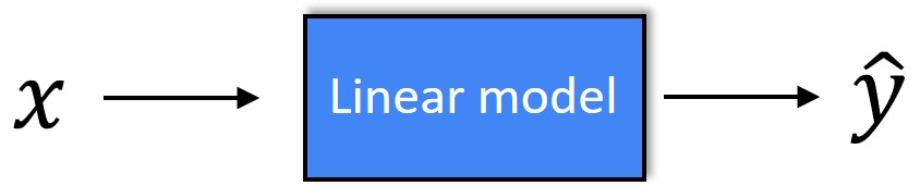
So, our first task is to design the model which takes an input $x $ and predicts the output $y $.

In this post we are going to examine a dataset that has a linear relationship. For example, if we want to predict a house price based on the size of the house, the size and price will commonly have a linear relationship. Another example can be the speed of the vehicle and the gasoline consumption. When the speed of a vehicle is low, the gasoline consumption will also be low. On the other hand, when the speed of a vehicle is high, the gasoline consumption will also be high.

Building a linear model

Let’s suppose that we want to find out if hardworking students receive higher grades. In that case we are going to analyze the dependence between the study time and grades. In the following image, the study time is shown along the $x $ axis, while the grades are shown along the $y $ axis.

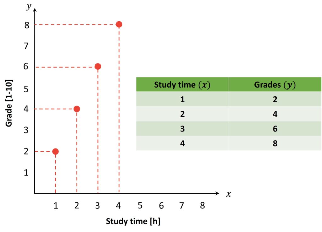
We can see that if study time in our imaginary example increases, grades should go up. On the other hand, if study time decreases grades should go down. Therefore, we can say that grades depend on how much time we spend learning. This is that reason why the variable represented along the $x $ axis is also called an independent variable and variable represented along the $y $ axis is called a dependent variable. We can also see that these variables have a positive correlation. On the other hand, we can also have the negative correlation if the independent variable is time spent on Instagram. In that case, when an independent variable increases the dependent variable will decrease.

Now if we have an input data for $x $ and $y $ we can draw a straight line that represents the correlation between these two variables. We call that line the regression line.

$$ y = xw+b $$

Now let’s brake down this formula. Here $y $ stands for a dependent value that needs to be predicted (grade). Then, $x $ is an independent variable (study time) that we use to predict our dependent value. Next, variable $w $ represents the slope of the line. As we have already explained, this slope can be either positive or negative depending on the relation between dependent and independent variable. Finally, we have the bias $b $ which is the point where $y $ axis and the regression line intercept.

So, we want to examine how study time affects grades. We will start the experiment by measuring the dependent and independent variable. These values represent coordinates of the points.

Now our goal is to apply Linear regression in order to model the relationship between a dependent variables and independent variables. To do that we can draw a line that best fits to our dataset. In that way, we can predict where the future points may be and we can also identify outliers.

However we have the problem. We can’t draw the line because the parameters $w $ and $b $ are unknown to us. Therefore, the main goal of our analysis is to determine the values for $w $ and $b $. In that way we will be able to find a function of a line which will determine the optimal correlation between dependent and independent variables in our model. Let’s see how we can do that.

2. Linear regression

To better understand the process of determining optimal parameters $w $ and $b $, let’s first try to guess them. First, we will guess the weight. We can say that $w_{1}=4 $ and draw the first line with that weight. Next, we can guess another weight $w=1 $ and draw the second line. Then, we will try to figure out which of these two lines is closer to the “true line”- defined with our data points. Note, that true value of $w $ is unknown, but lets assume for the moment that $w=2 $ and that our data have a linear relationship. This is called a process of learning and it is illustrated in the following example.

In the image above we can see three lines. The blue line is the true line, and we also have two lines with arbitrary weights. The equation of the line with the arbitrary weight can be written as:

$$ \hat{y} = xw+b $$

Here, $\hat{y} $ represents our prediction. In order to simplify our model we will ignore this bias for the moment.

Loss function

Now, our goal is to find the error between the true line and the line with the arbitrary coefficient. So, what is the error? It is the distance between the point with coordinates $(y,x) $ on the true line and the point with coordinates $(\hat{y},x) $ on the predicted line. So, we can easily calculate the error for both lines, and compare these results in order to see what error is smaller. In that way we will determine which of our two predictions is better.

Note that as a result of a difference $\hat{y} $ we can also get a negative value. So, in order to get the positive result we will square this value. The squared error is usually called the loss.

$$ loss=(\hat{y}-y)^{2} $$

Since the $\hat{y} = xw+b $ $(b=0 ) $, we can write our loss function in the following way:

$$ loss=(\hat{y}-y)^{2}=(xw-y)^{2} $$

So at the end of the process we want to minimize the loss.

Calculating the Mean Squared Error (MSE)

Now, let’s construct one experiment by using this loss function. We want to see how the loss will change using different values of $w $. To understand this take a look at the following example.

As you can see in the table above we computed losses for five different guesses: $w=0 $, $w=1 $, $w=2 $, $w=3 $ and $w=4 $. Then, we have calculated the mean of the loss. In statistics, this operation is called Mean Squared Error (MSE)and it measures the average of the squares of the errors. In other words, it is the average squared difference between the predicted values and the actual value. Usually, this MSE value represents the cost function.

The interesting case is one when $w=2 $ where mean of the loss is equal to 0. This indicates that the error between our prediction and the real value is equal to 0 and that we have predicted everything correctly.

So, we can express our loss/cost equation in the following way:

$$ cost=\frac{1}{N}\sum_{n=1}^{N}loss_{n} $$

$$ cost=\frac{1}{N}\sum_{n=1}^{N}(\hat{y}_{n}-y_{n})^{2} $$

Here, the cost is the sum of all loss data points divided by $N $ (the total number of all points). In other words, we can say that cost is the average of all loss values.

Cost graph

So, in the previous example we saw how we can manually calculate the optimal prediction for our model. Unfortunately, once we have a large number of weights, we cannot do this anymore. So we have to find some alternative way to identify the best prediction. In order to do that, let’s understand a relationship between cost and $w $ a little bit better. In the graph below we plotted the cost for all values of $w\in \left [ 0,4 \right ] $ in interval of 0 to 4, that we have calculated in the previous example.

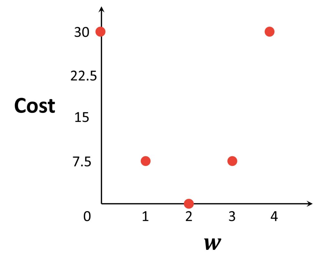
Now, if we connect these points we will see that our cost function is a convex parabola.

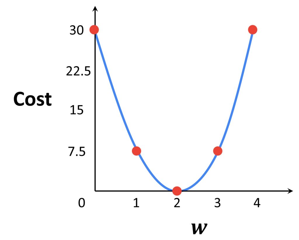
As you can see this function has a global minimum value when the value of $w $ is equal to 2 and the cost is equal to 0. This means that if we want to identify the weight value which minimizes the loss, we want to find a minimum of this function. To do this we will use the method called Gradient descent.

3. Gradient descent

Gradient descent is one of the most commonly used machine learning optimization methods. The goal of this algorithm is to minimize the cost function and to find optimal values for $w $ and $b $.

To better understand the Gradient descent algorithm let’s imagine that you are standing at the top of the hill on a foggy day. Your goal is to reach the point located at the base of the hill. Since the fog is very thick, you can not see that point, but you know that you need to move towards the base of the hill. So, you will begin to move downhill taking big steps when the slope of the hill is bigger, and small steps when the slope becomes smaller, until you reach that point.

The idea behind the Gradient descent algorithm is similar to the previous example. At the begging of the process Gradient descent does a few calculations when it is far away from the optimal solution, and increases the number of calculations when it is closer to the optimal value. To better understand this let’s take a look at the following image.

Suppose we have this kind cost of graph (cost is usually denoted by $J $). Since we don’t know what is the right value of $w $ we can just start with the random point. Let’s say that in our case initial $w $ is equal to 5. Next, when we choose the random point we have to decide in which direction we are going to move: left or right. The best way to decide this is to compute the gradient of this point and see if it is a positive or negative value. A gradient is a function that describes the slope of the tangent of the cost function.

$$ Gradient = \frac{dJ}{dw} $$

So, this means that if the gradient is positive we will move to the left and if the gradient is negative we will move to the right.

To analytically compute the gradient we can do the following derivative calculation:

$$ J=\frac{\mathrm{d}}{\mathrm{d} w}\left[(x w-y)^{2}\right] $$

$$ = 2(xw-y)\cdot \frac{d}{dw}\left [ xw-y \right ] $$

$$ =2\left(x \cdot \frac{\mathrm{d}}{\mathrm{d} w}w+\frac{\mathrm{d}}{\mathrm{d} w}-y\right)(x w-y) $$

$$ =2(1x+0)(xw-y) $$

$$ =2x(xw-y) $$

To update our gradient we also need to calculate by how much we need to move. We can do this by using the following formula:

$$ w: = w-\alpha \cdot \frac{dJ}{dw} $$

$$ = w-\alpha \cdot \frac{1}{N}\sum_{i=1}^{N} 2x^{(i)}(x^{\left ( i \right )}w-y^{\left ( i \right )}) $$

where $x^{(i)} $ and $y^{(i)} $ are the values of a single point measured data point.

Here we just subtracted our initial $w $ with the gradient. The parameter $\alpha $ (learning rate) will determine how much we need to move. It is usually a very small value ($\alpha=0.01 $).

So, based on this gradient, and $\alpha $ we will move to the left. Then, we will continue to compute the gradient moving towards the minimum value of $w $. Once our gradient is close to zero the algorithm will stop and we will know the minimum value of $w $. Hence, we computed the Global loss minimum.

In the following GIF animation the Gradient descent algorithm is visualized

Now, let’s see how we can create a linear regression model in Python using PyTorch.

4. Linear regression in PyTorch

We will start by applying an intuitive approach based on PyTorch, and then we will do a full implementation in PyTorch.

First, let’s import the necessary libraries including NumPy and matplotlib. We will also import torch, which is the PyTorch module.

import numpy as np
import matplotlib.pyplot as plt
import torchCode language: JavaScript (javascript)

Next, using the function np.array() we will create a variable named x_data which will be our intendent variable Also we will create a y_data variable, which will simply store the values of x_data multiplied by two.

x_data = np.array([1, 2, 3, 4, 5])
y_data = x_data * 2Code language: PHP (php)

Note that here we are using the same values as in the first example. The variable x_data represents the study time, and y_data represents the grades.

Now, we can scatter our data using the function plt.scatter(). As parameters we will pass the x_data and y_data variables.

plt.scatter(x_data, y_data)Code language: CSS (css)

Here we can see the relationship between $x $ and $y $. When $x $ is equal to 2 the $y $ is equal to 4.

Now, when we have defined our data, we can start off by creating the functions. First we will create a function named forward(), which will take three input parameters: $x $, $w $ which is weight, and $b $ which is bias. Next, we can create a variable named y_hat, by simply multiplying $x $ with the $w $ and then add the $b $. Here, we will also ignore $b $ due to the simplification.

def forward(x, w, b=0):
  y_hat = x * w + b
  return y_hatCode language: JavaScript (javascript)

The next function that we’re going to create is the loss function loss(). This function will take two parameters, y_hat and y. Remember that y_hat is the predicted value, while y is the true label, or the original value. Then, we will simply return the squared difference between y_hat and y.

This function will help us later on to calculate the Mean Squared Error (MSE).

def loss(y_hat, y):
  return (y_hat - y) ** 2Code language: JavaScript (javascript)

Now, we will visualize how the loss is changing depending on the weight. So, we will create a list called all_w and the list all_loss. In these two lists we will store all weight and all loss values. Then, we will create a for loop and use a function np.arange() which returns evenly spaced values within a given interval. As parameters we will put 0 – start of interval, 4 – end of interval, and 0.1 – spacing between values.

Next, we will create a temporary variable called l_sum which is set to be 0. Now, we will create another for loop to iterate through every value of x_data and y_data. Then, we will create a variable named y_hat in which we will store prediction values. To do that we’ll call the forward function that we have created in the previous step. As parameters we will pass in the x_data of i, and the $w $.

The next step is to create a variable l in which we will call the loss function. Here, we will pass the y_hat and the y_data of i. Then, we will simply add this l variable to the l_sum. Finally, we can append all calculated weights and losses to lists all_w and all_loss. Remember, the function loss is just calculating the squared error but not the mean squared error. So, we need to divide all calculated losses with the number of data points.

all_w = []
all_loss = []

for w in np.arange(0, 4, 0.1):
  l_sum = 0

  for i in range(len(x_data)):
    y_hat = forward(x_data[i], w)
    l = loss(y_hat, y_data[i])

    l_sum += l
  
  all_w.append(w)
  all_loss.append(l_sum / len(y_data))

Now when we have saved all weights and losses, we can create a stem plot and visualize them.

plt.stem(all_w, all_loss)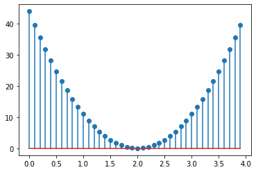Code language: CSS (css)

We can see that our weight is on the x-axis and on the y-axis is our loss. We can also see that as the weight approaches the value of 2 the loss is getting smaller and smaller. On the other hand, when the weight is moving away from the value of 2 it is getting bigger and bigger. So, we can say that the minimum of this function is at the point of 2.

Intuitive implementation of Linear regression in PyTorch

Now, we will apply an intuitive approach based on PyTorch. We will create a model for the linear regression. Because PyTorch is accepting only tensors, we need to convert our NumPy array of $x $ and $y $ data. So to do this, we will create a variable x_torch, and we will apply the torch.FloatTensor() function. As parameters we will pass in our variable x_data and we will reshape it in order to create a tensor. Then we’ll do the same thing for the y_data.

x_torch = torch.FloatTensor(x_data).reshape(-1, 1)
y_torch = torch.FloatTensor(y_data).reshape(-1, 1)

x_torch


tensor([[1.],
        [2.],
        [3.],
        [4.],
        [5.]])Code language: CSS (css)

y_torch


tensor([[ 2.],
        [ 4.],
        [ 6.],
        [ 8.],
        [10.]])Code language: CSS (css)

Now, we can create variables for weight and bias using the function torch.randn(). As parameters we will pass the value 1, which means that we want just one random number and we will set the parameter requires_grad to be True. This parameter is going to automatically compute the gradients for us.

Then, we will also do this for the bias.

w = torch.tensor(5., requires_grad=True)
b = torch.tensor(3., requires_grad=True)Code language: PHP (php)

Here we can define a learning rate to be equal to 0.05.

lr = 0.05

Now that we have defined our variables, we can start with the training. First we will create a for loop that will iterate in the range from 0 to 1000. That means that we will train our model 1000 epochs.

In the y_hat variable, we will store the result of the forward propagation. Once again, we can do the forward propagation by taking the $x $ values, multiplying them with the weight and adding the bias. After this, we need to calculate the MSE or the cost function. We can achieve this by using the function torch.sum().

Now, after the loss is computed, we need to apply the back propagation. We can do this by calling the loss.backward() function. This function will automatically compute the gradients for us.

Now, we need to set the criteria to calculate these gradients. First, we will turn them off with torch.no_grad() function. It is a context-manager that will disable gradient calculation, and free up some memory. Then, we will take the weight and subtract the product of the learning rate and the gradient for the weight. We will also do the same operation for the bias. Now to stop the accumulation of the gradients, we need to reset them before the next iteration . So, we can do this by taking the grad.zero_() function for $w $ and $b $.


for i in range(1000):
  y_hat = x_torch * w + b

  loss = torch.sum(torch.pow(y_torch - y_hat, 2) / len(y_torch))
  loss.backward()
  
  with torch.no_grad():
    w -= lr * w.grad
    b -= lr * b.grad

    w.grad.zero_()
    b.grad.zero_()Code language: JavaScript (javascript)

Since we have trained our model, we can take the results for weight and bias for it. To do that we will create a variable y_pred which will be equal to the product of x_torch and $w $ plus the bias.

y_pred = x_torch * w + b

Now, let’s see the prediction results for the $y $ and also the original results for $y $.

y_pred

tensor([[ 2.0000],
        [ 4.0000],
        [ 6.0000],
        [ 8.0000],
        [10.0000]], grad_fn=<AddBackward0>)Code language: HTML, XML (xml)

y_data

array([ 2,  4,  6,  8, 10])Code language: CSS (css)

We can see that they are equal. That means that our model guessed it correctly.

Let’s now plot this line. We will first plot the original values, and then, we will plot the predicted values. Note that y_pred is still a tensor and we need to convert it to a NumPy array. For that we will use the function .detach() to detach all grade gradients and then apply .numpy() to transform it into a NumPy array.

plt.plot(x_torch, y_torch, 'go')
plt.plot(x_torch, y_pred.detach().numpy(), '--')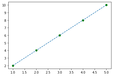Code language: JavaScript (javascript)

So, here we can see that the green dots are the original points, and the blue line is what our model predicted.

Now, you may be asking yourself, what’s the main goal of the output of this model? Well, the main goal of a linear regression model is to find a dependence between an independent variable, in this case x_torch, and the dependent variable, in this case y_torch. The main output of this model is the weight and the bias.

Here, we can check out the weight and bias.

w, b
(tensor(2.0000, requires_grad=True), tensor(7.2257e-07, requires_grad=True))Code language: PHP (php)

We can see that the weight is equal to 2, and the bias is some negative value. You may be asking now, how can we use this?

Well, let’s define the variable x_test by creating a tensor of one number, for example, 3.5. How can we find the y for this x_test? Well, we will grab the x_test, multiply it with the weight and add the bias.

x_test = torch.Tensor([3.5])

x_test * w + b


tensor([7.], grad_fn=<AddBackward0>)Code language: HTML, XML (xml)

We can see that the result is something close to 7 which is correct because it is doubled value of the x_test.

However, this is a very simple example. So, let’s create a more complex set of numbers, let’s say 50 numbers that are randomly generated. So, the following part of this post, we will fully implement linear regression model in Python.

So, what’s the next step? First we will create a more complex set of numbers. We can do this by using the np.random.rand() function that will create 50 numbers that are randomly generated in the interval between 0 an 1. Then, we will stretch the values of $x $ to the values in the interval between 0 to 10 by multiplying $x $ with 10.

x = np.random.rand(50)
x = x * 10

Now, we need to create the variable $y $. For example, we can say that one $y $ is equal to $x $ times 3 minus 4. We will also add some noise to the $y $. To do this we will use the np.random.rand() function again, create 50 random numbers and add them to our equation.

y = x * 3 - 4
y += np.random.randn(50)

Next step is to create a class called LinearModel(). To be able to use it as a PyTorch model, we will pass torch. nn.Module as a parameter. Now, we will define the init function or the constructor by passing parameter self.

class LinearModel(torch.nn.Module):
  def __init__(self):
    super(LinearModel, self).__init__()
    self.linear = torch.nn.Linear(1, 1)
  
  def forward(self, x):
    return self.linear(x)

Then we will call the super() function of the linear model. Note, that because this is a linear regression model, so it will have only one layer. That is why we will create a self. linear variable in which we’ll call the torch.nn.Linear() function. This function takes two input parameters. The first one is the size of each input sample. This parameter will be equal to 1 because we have only numbers. The second parameter is the shape of the output which will also be equal to 1. Now, we will create the forward() function which will take self and x as inputs. Finally, we will return self. linear and we’ll pass in $x $ as input.

Now we have created our linear model. Remember, PyTorch is accepting only tensors, so we need to convert our data to be tensors. We can achieve this by creating a variable x_torch, then call the function torch.FloatTensor(), and we pass $x $ as a parameter. We will also reshape this variable and we will do the same thing for $y $.

x_torch = torch.FloatTensor(x).reshape(-1, 1)
y_torch = torch.FloatTensor(y).reshape(-1, 1)

Now when we have defined our data, we can start coding the training part. We will start by creating a variable modelwhich will be used for calling our LinearModel class. Then, we will calculate the loss by using the function torch.nn.MSELoss(). With this function we will calculate the mean squared error.

Now, remember that in the previous part of the code, we updated the weight and the bias by hand. Now, we want to let PyTorch to do the heavy lifting. So, we will create a variable named optimizer, and call the function torch.optim.SGD()which will calculate the gradients. SGD stands for Stochastic Gradient Descent. Then, we will pass the parameters that we want to update – the weight and the bias. So, as parameters to this function, we will pass the model.parameters(), and the learning rate which will be equal to 0.01.

model = LinearModel()
criterion = torch.nn.MSELoss()
optimizer = torch.optim.SGD(model.parameters(), lr=0.01)

The next step is to train of our model. First we will create a for loop that will iterate in the range from 0 to 1000.

The first step in the training loop is predicting or the forward pass. So, we will create the variable y_hat and call the model on x_torch variable. Next, we need to calculate the loss which is equal to the criterion of the predicted value y_hat and original value y_torch.

After the loss is calculated we need to do the backward propagation. Now, to calculate the gradients we will just call the optimizer.step() function which will update the weight and the bias for us. Also, we need to make sure that the calculated gradient is equal to 0 after each epoch. To do that, we’ll just call optimizer.zero_grad() function.

all_loss = []

for epoch in range(1000):
  y_hat = model(x_torch)

  loss = criterion(y_hat, y_torch)
  loss.backward()
  all_loss.append(loss.item())

  optimizer.step()
  optimizer.zero_grad()

Now, let’s make some predictions with the model.forward() function

y_pred = model.forward(x_torch)

Here, we can plot our results.

plt.plot(x_torch, y_torch, 'go')
plt.plot(x_torch, y_pred.detach().numpy(), '--')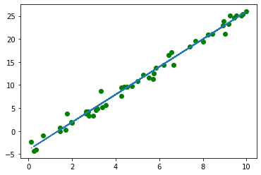Code language: JavaScript (javascript)

We can clearly see that this line goes in between all original points.

Let’s now print the calculated values for the weight and the bias. We will do that by simply creating the following for loop which will return the final results of weight and the bias for this model.

for name, param in model.named_parameters():
  print(name, param)Code language: CSS (css)

linear.weight Parameter containing:
tensor([[3.0017]], requires_grad=True)
linear.bias Parameter containing:
tensor([-4.0587], requires_grad=True)Code language: PHP (php)

We can see that the weight has a value of 3.0017, and the bias has a value of -4.0584. If we check how we created our $y $ variable, we will see that the weight is equal to 3 and the bias is equal to -4. That means that we obtained correct results.

This is a nice way to visualize the prediction. However, we want to track the model’s performance. So we’ll go back to the training iterations. And we will create a list all_loss[]. Then, and after each loss calculation, we will append loss to that list. As a parameter we will pass the loss.item because we want just the number.

Here, we can plot our result. On the x-axis we’ll create a list ranging from zero to 200, and we’ll also plot the loss for the first 200 numbers.

plt.plot(np.arange(0, 200, 1), all_loss[:200])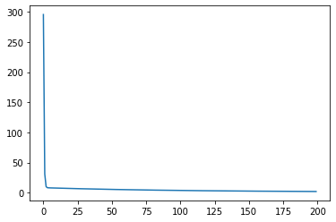Code language: CSS (css)

We can see that in the beginning, the loss had a massive drop, but then at some point it became pretty stable. Now, let’s check out the first 10 numbers.

all_loss[:100]Code language: CSS (css)

[354.6148681640625,
 33.66743087768555,
 8.063434600830078,
 5.989849090576172,
 5.791196823120117,
 5.74216365814209,
 5.705296039581299,
 5.669642448425293,
 5.634324550628662,
 5.599271774291992]Code language: JSON / JSON with Comments (json)

We can see that first number of loss was 354, then it dropped all the wat to 33, then to 8. After the third step we can see that loss is still drooping but at much smaller rate. Let’s now print the last number from this list.

all_loss[-1]Code language: CSS (css)

0.9462018013000488Code language: CSS (css)

So, we can se that the loss continue to drop until it reached the number of 0.946.

Click here to get PyTorch code !

Summary

That is it for this post where we talked about Linear regression. First we explained a theory behind this method. You learned how to build a linear regression model, how to calculate the error, loss and the cost of that model. Then, we learned how to use the Gradient descent algorithm to automatically calculate the global minim. Finally, we implemented that knowledge into using PyTorch. In the next post we will focus a little bit more on the mathematics and learn how to use automatic differentiation Autograd in PyTorch.

#003 PyTorch – How to implement Linear Regression in PyTorch