#003B Gradient Descent
Gradient Descent
A term “Deep learning” refers to training neural networks and sometimes very large neural networks. They are massively used for problems of classification and regression. The main goal is to optimize parameters \( w \) and \( b \) ( both in logistic regression and in neural networks ).
Gradient Descent achieved amazing results in solving these optimization tasks.
Not so new, developed in the
Hence, Gradient Descent is an algorithm that tries to minimize the error (cost) function \(J(w,b)\) and to find optimal values for \(w\) and \(b\).
Gradient descent algorithm has been used to train and also learn the parameters \(w \) and \(b\) on a training set.
How does Gradient Descent Work?
Gradient Descent starts at an initial parameter and begins to take values in the steepest downhill direction. Function \(J(w,b) \) is convex, so no matter where we initialize, we should get to the same point or roughly the same point.
After a single step, it ends up a little bit down and closer to a global otpimum because it is trying to take a step downhill in the direction of steepest descent or quickly down low as possible.
After a fixed number of iterations of Gradient Descent, hopefully, will converge to the global optimum or get close to the global optimum.
The learning rate \( \alpha \) controls how big step we take on each iteration of Gradient Descent.
Derivative, slope of a function at the point, is basically the update of the change you want to make to the parameters \(w\). Note that in our code ” \(
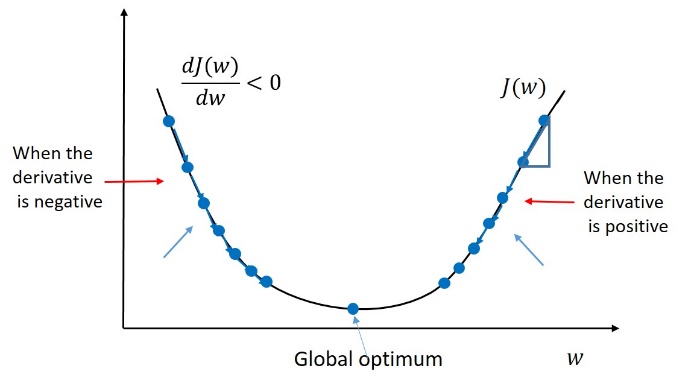
Explanation of the graph:
If the derivative is positive, \(w \) gets updated as \(w \) minus a learning rate \( \alpha \) times the derivative ” \(dw\) “.
We know that the derivative is positive, so we end up subtracting from \(w \) and taking a step to the left. Here, Gradient Descent would make your algorithm slowly decrease the parameter if you have started off with this large value of \(w \).
Next, when the derivative is negative (left side of the convex function), the Gradient Descent update would subtract \( \alpha \) times a negative number, and so we end up slowly increasing \(w \) and we are making \(w \) bigger and bigger with each successive iteration of Gradient Descent.
So, whether you initialize \(w \) on the left or on the right, Gradient Descent would move you towards this global minimum.
Hence note: If \(J \) is a function of two variables, we will use the lower case \(d \), instead to use the partial derivative symbol – \( \partial \).
These equations are equivalent:
.
| \( w = w – \alpha \frac{\mathrm{d} J(w,b) }{\mathrm{d} w} \) | \( b = b – \alpha \frac{\mathrm{d} J(w,b) }{\mathrm{d} b} \) |
| \( w = w – \alpha \frac{\partial J(w,b) }{\partial w} \) | \( b = b – \alpha \frac{\partial J(w,b) }{\partial b} \) |
In the next post will we demonstrate an implementation of gradient descent in python.


