CamCal #012 Stereo Geometry Code
Highlights: In this post we will finish our mini series on stereo geometry. We will wrap some things up, and go through the code related to this.
In the last few posts we talked about stereo geometry. We covered many concepts, from basic stuff, such as essential matrix and epipolar lines to the fundamental matrix. Here, we will present a code that can help us to compute them.
Tutorial Overview:
- Detecting key points (SIFT, SURF, ORB)
- Matching key points
- Computing a fundamental matrix
- Computing epipolar lines
- An ideal stereo system
1. Detecting key points
Motivation: Earlier we talked about the Harris operator, but the problem with this operator is that it is not invariant to scale. Another drawback is that when we find a point on two images, the question is how do we match them? How do we determine which points in the first image are the same as points in the second image. So to do this, we need what is referred to as a descriptor. A descriptor is a description of the neighborhood where the interest point is, and that will allow us to match these points.
However, we want this descriptors to be invariant. This means that it should be almost the same on both images. It would be great if they were exactly the same, and also they should be unique.
Hence, we also need the descriptors do be distinctive. Distinctive means that a point in one image has only one descriptor in the other image. Moreover, a different point would have a different descriptor.
So, we have this tradeoff between: being invariant, that it is found each time, and being distinctive.
SIFT
SIFT stands for Scale Invariant Feature Transform and it was developed in 1999 and early 2000s. Motivation for its development was that the Harris operator is not invariant to scale as we have mentioned earlier. The goals of SIFT development were to develop an interest operator (a detector) that is invariant to scale and rotation and also to create a descriptor that was robust to the variations corresponding to typical viewing conditions. It is important to say that this descriptor is is mostly used.
Furthermore, the idea is that if we can find enough matches, then we can figure out whether the object is found in both images. In addition, an object the object in the other image can be rotated, translated and maybe scaled. Hence, the overall SIFT procedure looks like this:
- Scale-space extrema detection
- Keypoint localization
- Orientation assignment
- Build a descriptor
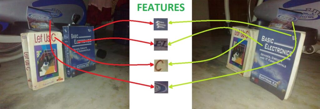
SURF
Six years after SIFT has been introduced, three researchers published another paper where SURF descriptors have been invented, which stands for Speeded Up Robust Features. It is a speeded-up version of the SIFT algorithm. The main difference here is that instead of using the difference of Gaussian approach as SIFT, SURF uses Hessian matrix approximation to detect interesting points and use the sum of Haar wavelet responses for orientation assignment. We will not dive deeper into this, and more resources for this will be provided at the end of this post.
But, SIFT and SURF are actually patented and they are removed from newer versions of OpenCV, so a new method must be used. For that purpose we introduce an ORB.
ORB
Oriented Features from Accelerated Segment Test and Rotated Binary Robust Independent Elementary Features (Oriented FAST and Rotated BRIEF). We will just call it ORB algorithm that came out from OpenCV labs and it is not patented.
ORB is a good alternative to SIFT and SURF, while being also computationally efficient. ORB is a combination of FAST keypoint detector and BRIEF descriptor with many modifications to boost the performance. We will use ORB in the rest of this post.
Fist part of ORB algorithm is to use FAST detector to locate features. FAST features are not computational heavy, but have few shortcomings. That is, they tend to respond to edges and corners, so in order to fix this, ORB computes the Harris corner measure for located points. The Harris corner measure provides a better metric for feature selection and it is used to select the best features in an image. Difference between ORB and FAST is that ORB algorithm uses an orientation for keypoints. An orientation is assigned by first computing the gradients in both directions inside the box around the feature. So, once the feature has been located and an orientation has been assigned, it is possible to compute a feature vector relative to that orientation. Then, the resulting feature can be used in a rotationally invariant ways.
A difference between the ORB and BRIEF features is that BRIEF’s authors actually produced the rotation-aware BRIEF descriptor by analyzing a set of images and looking for test pairs that had particular properties. In contrast, this analysis was done once during the construction of the ORB descriptor, and, as such, it was built into the descriptor in OpenCV.
Finally, it is worth mentioning that all of these algorithms are implemented in OpenCV via the Feature2D interface.
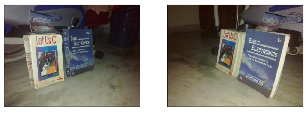
So, let’s start with these two pictures. This is just a basic example.
Python
C++
#include <opencv2/opencv.hpp>
#include <iostream>
#include <opencv2/features2d.hpp>

using namespace std;

int main()
{
    // Loading the actual image
    cv::Mat image_left, image_right;

    image_left=imread("left.jpg", cv::IMREAD_COLOR);
    cv::imshow("Left image", image_left);
    cv::waitKey();

    image_right=imread("right.jpg", cv::IMREAD_COLOR);
    cv::imshow("Right image", image_right);
    cv::waitKey();

    // Converting the color image into grayscale
    cvtColor(image_left, image_left, cv::COLOR_BGR2GRAY);
    cvtColor(image_right,image_right,cv::COLOR_BGR2GRAY);

    // Vector of keypoints
    std::vector<cv::KeyPoint> keypoints1;
    std::vector<cv::KeyPoint> keypoints2;

    // We will use orb feature detector
    // Construction of the orb feature detector
    cv::Ptr<cv::FeatureDetector> orb = cv::ORB::create(5000);

    // Feature detection
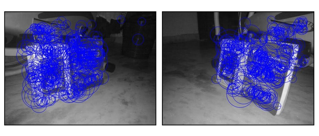
    orb->detect(image_left, keypoints1);
    orb->detect(image_right,keypoints2);

    // Draw the kepoints
    cv::Mat imageKeyPoints;
    // Left image
    cv::drawKeypoints(image_left, keypoints1, imageKeyPoints, cv::Scalar(0, 0, 255),
                      cv::DrawMatchesFlags::DRAW_RICH_KEYPOINTS);
    cv::imshow("Left image", imageKeyPoints);
    cv::waitKey();
    // Right image
    cv::drawKeypoints(image_right, keypoints2, imageKeyPoints, cv::Scalar(0, 0, 255),
                      cv::DrawMatchesFlags::DRAW_RICH_KEYPOINTS);
    cv::imshow("Right image", imageKeyPoints);
    cv::waitKey();

    // Extraction of the orb descriptors
    cv::Mat descriptors1, descriptors2;
    orb->compute(image_left, keypoints1, descriptors1);
    orb->compute(image_right, keypoints2, descriptors2);
2. Matching key points
Finally, we have these feature points, or to say, descriptors. Now, it is time to match them. In more simpler words, we need to find them in both images, or more. For now, just two.
So, SIFT and SURF are usually matched using the Euclidean distance. SIFT and SURF descriptors represent the histogram of oriented gradient (of the Haar wavelet response for SURF) in a neighborhood, alternatives of the Euclidean distance are histogram-based metrics. But, ORB which is a binary descriptor should be matched using the Hamming distance.
$$ d_{hamming}(a,b)=\sum_{i=0}^{n-1}(a_{i} \oplus b_{i}) $$
Basically, this is the distance that is equivalent to the number of different elements for binary strings. To sort matches, we will use a distance ratio test which is proposed by Lowe and it is known as Lowe’s ratio test. The idea is that for a good match the distance between two nearest matches for a certain keypoint is below a threshold, or vice versa.
Python
C++
cv::FlannBasedMatcher matcher = cv::FlannBasedMatcher(cv::makePtr<cv::flann::LshIndexParams>(6, 12, 1),cv::makePtr<cv::flann::SearchParams>(50));
    std::vector< std::vector<cv::DMatch> > matches;
    matcher.knnMatch(descriptors1, descriptors2, matches, 2 );

    std::cout<<"matches size: "<<matches.size()<<std::endl;
    // Select few Matches
    std::vector<cv::DMatch> good;

    //Filter matches using the Lowe's ratio test
    const float ratio_thresh = 0.7f;
    for (size_t i = 0; i < matches.size(); i++){
        if (matches[i].size() >= 2){
            if (matches[i][0].distance < ratio_thresh * matches[i][1].distance){
                good.push_back(matches[i][0]);
            }
        }
    }

    cout<< "Number of matched points: " << good.size() << endl;
3. Computing a fundamental matrix
Here, we won’t repeat again the whole procedure of finding the fundamental matrix. However, just keep in mind what it is and remember the following equation. Luckily for us, OpenCV has a function for this. It is called findFundamentalMat.
A fundamental matrix relates pixel coordinates in two views from two cameras, and it is more general form than an essential matrix. So with this, we remove the need to know intrinsic parameters.
$$ p^{T}Fp’=0 $$
Python
C++
// Convert one vector of keypoints into two vectors of Point2f
    std::vector<int> points1;
    std::vector<int> points2;
    for (auto iter = good.begin(); iter != good.end(); ++iter){
        // Get the indexes of the selected matched keypoints
        points1.push_back(iter->queryIdx);
        points2.push_back(iter->trainIdx);
    }

    // Convert keypoints into Point2f
    std::vector<cv::Point2f> selPoints1, selPoints2;
    cv::KeyPoint::convert(keypoints1, selPoints1, points1);
    cv::KeyPoint::convert(keypoints2, selPoints2, points2);


    // Compute F matrix from all good matches
    cv::Mat fundemental = cv::findFundamentalMat(cv::Mat(selPoints1), cv::Mat(selPoints2), cv::FM_LMEDS);

    std::cout << "F-Matrix size= " << fundemental.rows << "," << fundemental.cols << std::endl;
    std::cout << "F-Matrix = \n" << fundemental << std::endl;
And this is how our fundamental matrix looks like:
-4.28884209e-06  3.66651364e-05 -1.91119719e-04
 4.96146550e-05 -2.36601500e-06 -3.82250734e-02
-3.10154182e-03  1.46422833e-02  1.00000000e+00
4. Computing epipolar lines
So now, when we have fundamental matrix computed, we can find epipolar lines. This can be done using these equations:
$$ l = Fp’ $$
is the epipolar line in the \(\Pi\) image associated with \(\Pi’\). And
$$ l’ = F^{T}p $$
is the epipolar line in the prime image associated with \(\Pi\).
Python
C++
// Draw the left points corresponding epipolar lines in right image
    std::vector<cv::Vec3f> lines1;
    cv::computeCorrespondEpilines(cv::Mat(selPoints1), 1,  fundemental, lines1);
    for (auto iter = lines1.begin(); iter != lines1.end(); ++iter){
        cv::line(image_right, cv::Point(0, -(*iter)[2] / (*iter)[1]),
                 cv::Point(image_right.cols, -((*iter)[2] + (*iter)[0] * image_right.cols) / (*iter)[1]),
                 cv::Scalar(255, 255, 255));
    }

    // Draw the RIGHT points corresponding epipolar lines in left image
    std::vector<cv::Vec3f> lines2;
    cv::computeCorrespondEpilines(cv::Mat(selPoints2), 2, fundemental, lines2);
    for (auto iter = lines2.begin(); iter != lines2.end(); ++iter){

        cv::line(image_left, cv::Point(0, -(*iter)[2] / (*iter)[1]),
                 cv::Point(image_left.cols, -((*iter)[2] + (*iter)[0] * image_left.cols) / (*iter)[1]),
                 cv::Scalar(255, 255, 255));
    }

    // Display the images with points and epipolar lines
    cv::imshow("Left Image", image_left);
    cv::waitKey();
    cv::imshow("Right Image", image_right);
    cv::waitKey();

    return 0;
}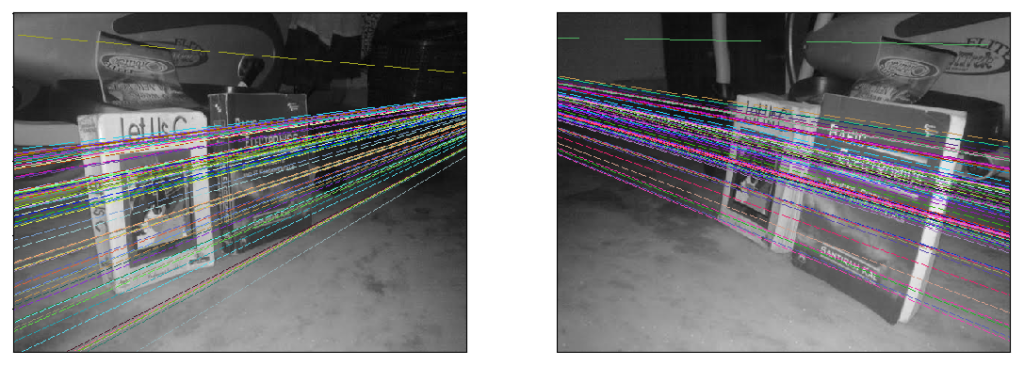
A fundamental Matrix estimation is sensitive to quality of matches and outliers. If case that all scene points lie on a plane, or if the camera has undergone a pure rotation (no translation), we have a big problem. So, we need to be careful.
5. An ideal stereo system
In the last example, we had an image where epipolar lines are converging to an epipole. However, if we have a perfect stereo system (cameras are only translated, whereas there was no rotation), we will have epipolar lines that are parallel to each other. Let’s see this example.
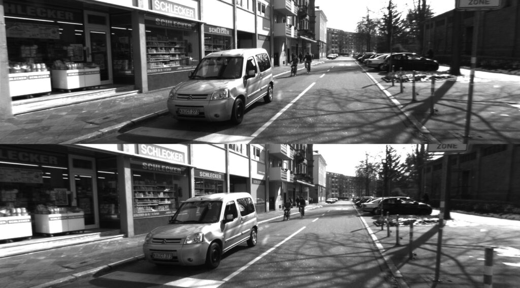
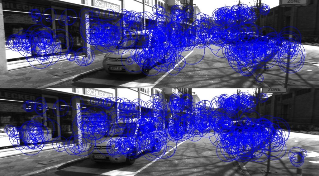
And when we compute descriptors it looks like this:
And finally we can see epipolar lines:
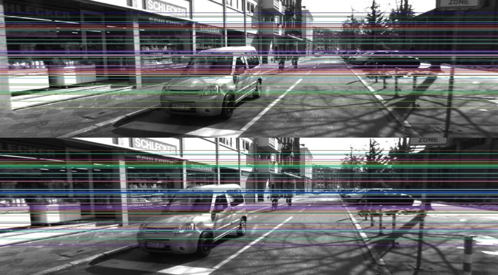
From the above picture, we can easily conclude that we have an ideal stereo system, so that means that we have two cameras whose image planes are exactly coplanar with each other with exactly parallel optical axes. This can be very useful when computing depth.
Summary:
Finally, when we know how to compute fundamental matrix and epipolar lines, we can start talking about depth estimation. So this will be our next post.