OpenCV #006 Sobel operator and Image gradient
Digital Image Processing using OpenCV (Python & C++)
Highlights: In this post, we will learn what Sobel operator and an image gradient are. We will show how to calculate the horizontal and vertical edges as well as edges in general.
What is the most important element in the image? Edges! See below.
Tutorial Overview:
1. What is the Gradient?
Let’s talk about differential operators. When differential operators are applied to an image, it returns some derivative. These operators are also known as masks or kernels. They are used to compute the image gradient function. And after this has been completed, we need to apply a threshold to assist in selecting the edge of pixels.
And what is then multivariate? Multivariate means that a function is actually a function of more than one variable. For example, an image is a function of two variables, \(x \) and \(y \). When we have functions that are a function of more than one variable, we refer to it as a partial derivative. Which is the derivative in the \(x \) or in the \(y \) direction. And the gradient is the vector that’s made up of those derivatives.
$$ \bigtriangledown f= \left [ \frac{\partial f}{\partial x},\frac{\partial f}{\partial y} \right ] $$
So what operator are we going to use in showing the gradient? It’s the vector above.
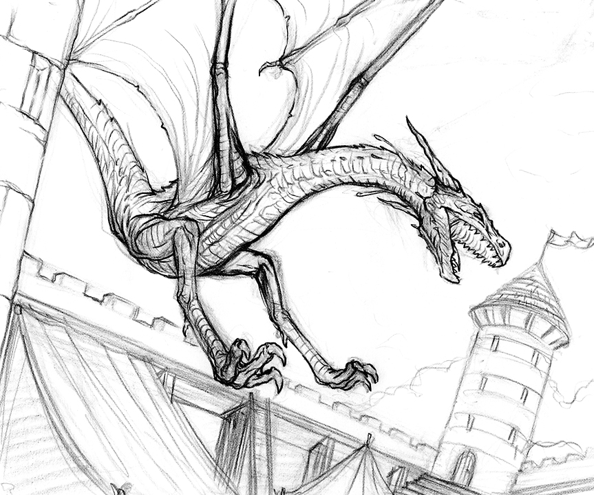
If we recall, what an image is. It is a two vector, made up \(\partial f \) with respect to \(x \), (The gradient of the image in the x direction) and the \(\partial f \) with respect to \(y \).
\(\partial f \) respect to \(x \)
Base on the vector above, the image only changes in the x-direction. So, the gradient would be whatever the changes are in the x-direction and \(0 \) in the y-direction. The same method can be applied to the changes in the y-direction.
We have explained horizontal and vertical edge detectors before. You can find more about it in posts CNN002 and CNN003.
Python
C++
#include <iostream>
#include <opencv2/opencv.hpp>

using namespace std;
using namespace cv;

int main()
{

    Mat image = cv::imread("truck.jpg", IMREAD_GRAYSCALE);
    cv::imshow("Truck", image);
    cv::waitKey();

    // we have already explained linear filters for horizontal and vertical edge detection
    // reference -->> CNN #002, CNN #003 posts.

    cv::Mat image_X;
    // this is how we can create a horizontal edge detector
    // Sobel(src_gray, dst, depth, x_order, y_order)
    // src_gray: The input image.
    // dst: The output image.
    // depth: The depth of the output image.
    // x_order: The order of the derivative in x direction.
    // y_order: The order of the derivative in y direction.
    // To calculate the gradient in x direction we use: x_order= 1 and y_order= 0.
    // To calculate the gradient in x direction we use: x_order= 0 and y_order= 1.
    cv::Sobel(image, image_X, CV_8UC1, 1, 0);
    cv::imshow("Sobel image", image_X);
    cv::waitKey();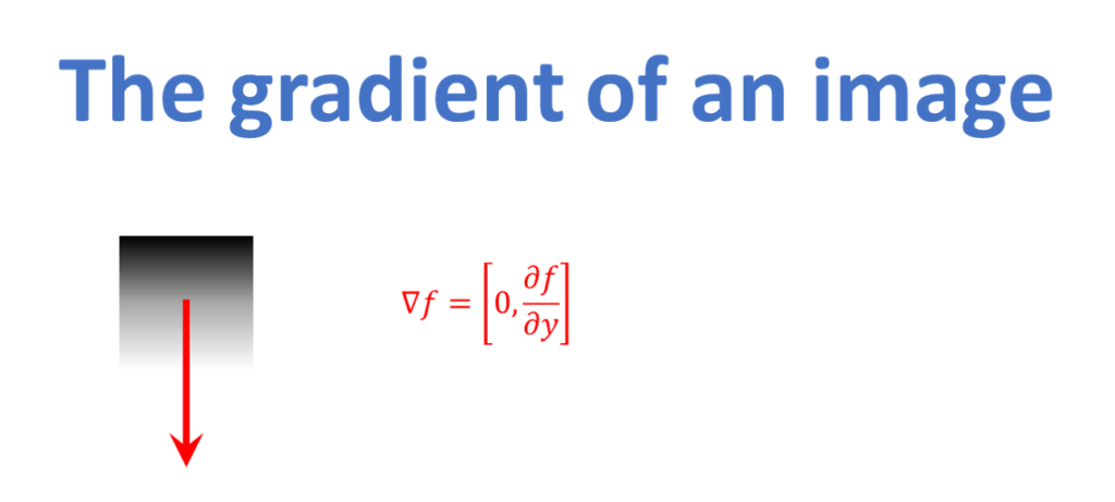
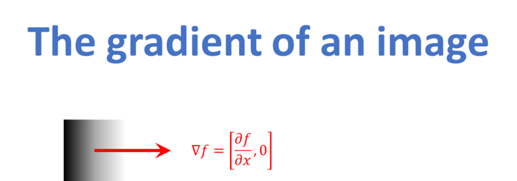
\(\partial f \) respect to \(y \)
As we can see, the direction of the gradient in y is getting more positive as you go down. In the sense that, it’s getting brighter in this direction. So in our image, the gradient would be 0, \(\partial f \) respect to \(x \), yet, we would have \(\partial f \) respect to \(y \).
Python
C++
    cv::Mat image_Y;
    // this is how we can create a vertical edge detector.
    cv::Sobel(image, image_Y, CV_8UC1, 0, 1);
    cv::imshow("Sobel image", image_Y);
    cv::waitKey();
And, of course we have changes in both directions and that’s the gradient itself.
It’s \(\partial f \) respect to \(x \), and the \(\partial f \) respect to \(y \). It has both magnitudes, which shows how things are getting brighter. And also an angle \(\theta \) that represents the direction the intensity is increasing. Here we are just expressing all of this.
Python
C++
    // When we combine the horizontal and vertical edge detector together
    cv::Mat sobel = image_X + image_Y;
    cv::imshow("Sobel - L1 norm", sobel);
    cv::waitKey();
The gradient of an image – Here, the gradient is given by the two partial derivatives. \(\partial f \) respect to \(x \), and the \(\partial f \) respect to \(y \).
$$ \bigtriangledown f= \left [ \frac{\partial f}{\partial x},\frac{\partial f}{\partial y} \right ] $$
The gradient direction is given by – The direction can be computed by computing the arctangent. This is the arctan of the changes in \(y \) over the change in \(x \). Sometimes, it’s also recommended to use atan2. So if the \(\partial f \) with respect to \(x \) is zero, that your machine doesn’t explode.
$$ \theta = tan^{-1}\left ( \frac{\partial f}{\partial y}/\frac{\partial f}{\partial x} \right ) $$
The amount of change is given by the gradient magnitude – This shows us how rapidly the function is changing, which is very much related to finding edges by looking for large magnitudes of gradients on the image.
$$ \left \| \bigtriangledown f \right \|= \sqrt{\left ( \frac{\partial f}{\partial x} \right )^{2}+\left ( \frac{\partial f}{\partial y} \right )^{2}} $$
2. Finite Differences
The above calculus story is just fine. However, how do we compute the gradients in our images because we work with discrete variables and not with continuous ones. Let’s see more about discrete gradients:
$$ \frac{ \partial f\left ( x,y \right )}{\partial x}= \lim_{\varepsilon \rightarrow 0}\frac{f\left ( x+\varepsilon ,y \right )-f\left ( x,y \right )}{\varepsilon } $$
In continuous math, the partial derivative \(\partial f \) with respect to \(x \) is this limit. So we move a little bit in the \(x \) direction, subtract off the original one and divide by \(\varepsilon \). Meanwhile, when the limit reaches zero, that becomes our derivatives.
In the discrete world, we can’t move closer. We have to take the finite difference.
$$ \frac{ \partial f\left ( x,y \right )}{\partial x}\approx \frac{f\left ( x+1,y \right )-f\left ( x,y \right )}{1 }\approx f\left ( x+1,y \right )-f\left ( x,y \right ) $$
When approximating our partial by finite difference. We take one step in the \(x \) direction, then subtract off the original and divide by \(1 \). Since that’s how big of a step we took.
So that’s become the value \(f\left (x+1,y \right )-f\left ( x,y \right ) \) . In other words, this is called the right derivative because it takes one step to the right. For instance, let’s take a closer look at our finite differences, to think about these derivatives the right way.
A simple illustration of finite difference.
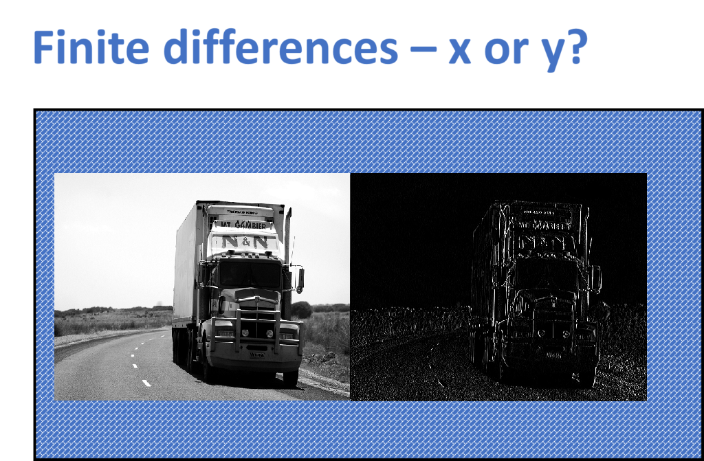
We have a picture of this truck. This is a good illustration of those finite difference images. First question, is this the finite difference in \(x \) or in \(y \)? Let’s have a look.
Going through the image in the \(x \)-direction, we get some kind of transition between these vertical stripes. To clarify, we get a change from bright values, to dark values, then bright values again, across the image horizontally.
In addition, we can hardly see any changes in \(y \), but only in \(x \). Hence, this is going to be a finite difference in \(x \).
The image we are presenting contains both negative and positive numbers. When showing an image, we make black-0, and other numbers white. However, it is preferable to say some minimum values are black, and some maximum is white. So we can make \(-128 \) to be black, \(+ 127 \) to be white. The in-between values will be gray (also zero values).
3. The Discrete Gradient
How do we pick an “operator” (mask/kernel) that can be applied to any image to implement these gradients? Well, here is an example below of an operator \(H \).
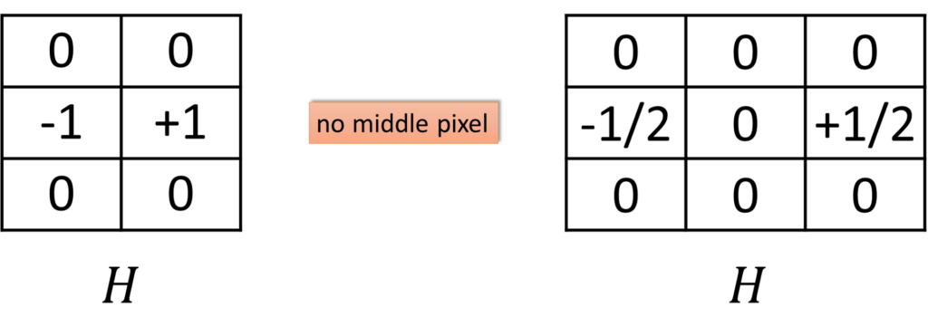
So looking at this operator, with 3 rows and 2 columns above. Is this a good operator? Well, you figured it. NO!!!.
Why is that? One reason is there are no middle pixel values.
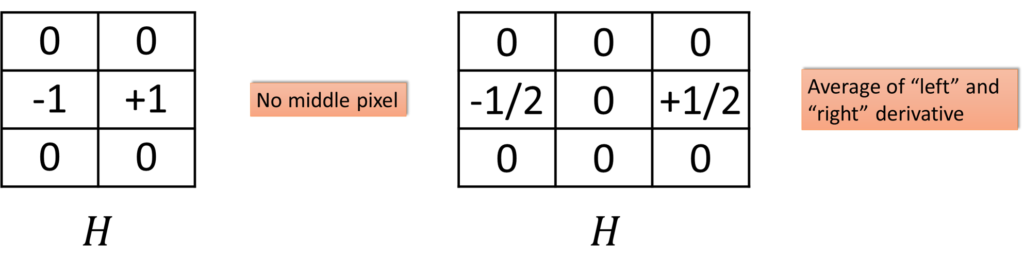
Now you might ask yourself, why is it a plus half and minus a half? Um… A good question, only if you did wonder why.
It is the average or normalization of the right derivative and the left derivative. The right derivative would be a \(+1 \) at the right of the kernel, and \(-1 \) at the middle. The left derivative would be a \(+1 \) at the left of the kernel, and \(-1 \) at the middle.
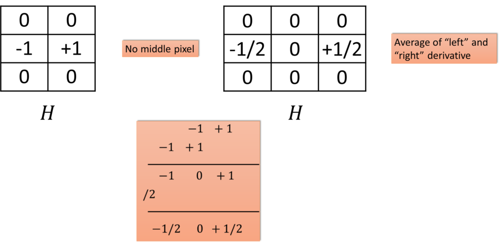
Average of “left” and “right” derivative
To get the average, we would add them and divide by two. Which is the sum. So, we get \(-1 \) (left), \(0 \) (middle), \(1 \) (right). Then when we divided by two to get \(-\frac{1}{2} \) (left), \(+\frac{1}{2} \) (right) with a \(0 \) in the middle.
4. Sobel Operator
The most common filter for doing derivatives and edges is the Sobel operator. It was named after \(Irwin Sobel\) and \(Gary Feldman \), after presenting their idea about an “Isotropic 3×3 Image Gradient Operator” in 1968. The operator looks like the image below.
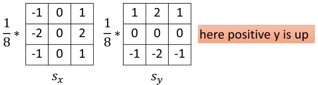
But instead of \(-\frac{1}{2} \) and \(+\frac{1}{2} \), it’s got this weird thing where it’s doing these eighths. And you can see that it does, not only \(+2 \), \(-2 \), which we would then divide by \(4 \) and we get the same value. But it also does a \(+1 \), \(-1 \) on the row above, and below the row.
The idea is, to compute a derivative at a pixel, we won’t look left, and right at ourselves but also look nearby.
Another equation to be familiar with
By the way, the \(y \) is here as well, and in this case, \(y \) is positive going up. Remember, it can go in either direction.
Sobel gradient is: Made up of the application of this \(s_ {x} \) and \(s_ {y} \) to get us these values.
$$ \bigtriangledown I= \begin{bmatrix}g_{x} & g_{y}\end{bmatrix}^{T} $$
The gradient magnitude: Is the square root of the sum of squares.
$$ g= \left ( g_{x}^{2}+g_{y}^{2} \right )^{1/2} $$
The gradient direction: Is what we did before. And here, it is \(arctan2 \) we were talking about to get the gradient.
$$ \theta = atan2\left ( g_{y},g_{x} \right ) $$
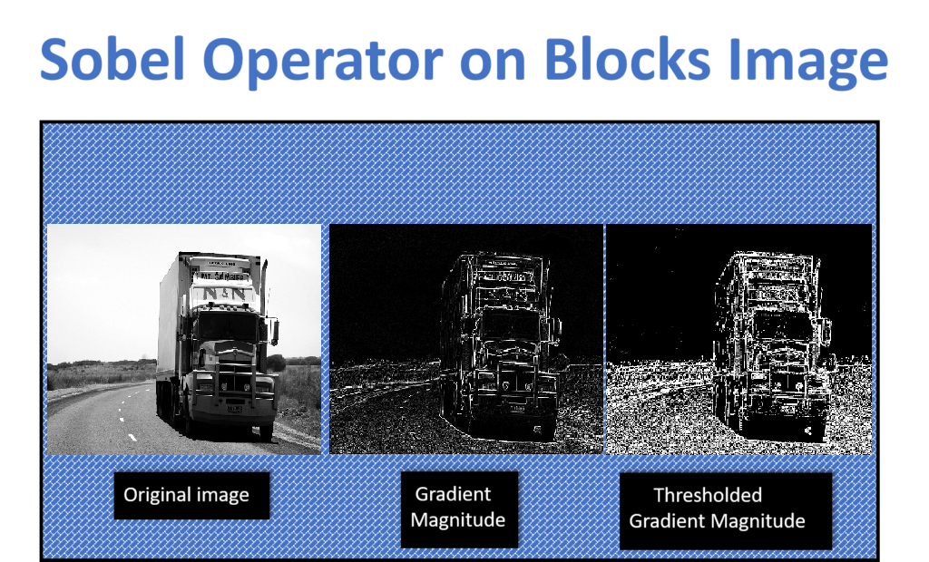
Here is an example. The picture on the left is an image. The one in the middle is a gradient magnitude. We applied the Sobel operator, then took the square root of the sum of squares. Then threshold it. And you will notice two things. One, it’s not an awful edge image and it’s not a great edge image. So we are partly towards getting that done.
Python
C++
// this idea is inspired from the book
    // "Robert Laganiere Learning OpenCV 3:: computer vision"
    // what it actually does, makes the non-edges to white values
    // and edges to dark values, so that it is more common for our visual interpretation.
    // this is done according to formula
    // sobelImage = - alpha * sobel +  255;
    double sobmin, sobmax;
    cv::minMaxLoc(sobel, &sobmin, &sobmax);

    cv::Mat sobelImage;
    sobel.convertTo(sobelImage, CV_8UC1, -255./sobmax, 255);
    cv::imshow("Edges with a sobel detector", sobelImage);
    cv::waitKey();


    cv::Mat image_Sobel_thresholded;
    double max_value, min_value;
    cv::minMaxLoc(sobelImage, &min_value, &max_value);
    //image_Laplacian = image_Laplacian / max_value * 255;


    cv::threshold(sobelImage, image_Sobel_thresholded, 20, 255, cv::THRESH_BINARY);
    cv::imshow("Thresholded Sobel", image_Sobel_thresholded);
    cv::waitKey();
// Also, very popular filter for edge detection is Laplacian operator
// It calculates differences in both x and y direction and then sums their amplitudes.
cv::Mat image_Laplacian;
// here we will apply low pass filtering in order to better detect edges
// try to uncomment this line and the result will be much poorer.
cv::GaussianBlur(image, image, Size(5,5), 1);
cv::Laplacian(image, image_Laplacian, CV_8UC1);
cv::imshow("The Laplacian", image_Laplacian);
cv::waitKey();
cv::Mat image_Laplacian_thresholded;
double max_value1, min_value1;
cv::minMaxLoc(image_Laplacian, &min_value1, &max_value1);
//image_Laplacian = image_Laplacian / max_value * 255;
cv::threshold(sobel, image_Laplacian_thresholded, 70, 220, cv::THRESH_BINARY);
cv::imshow("Thresholded Laplacian", image_Laplacian_thresholded);
cv::waitKey();
return 0;
}Summary
If you are just starting with an image processing, this post gave you insights on how we can calculate image gradients. We will use these ideas heavily in image processing and they will assist us in how to detect edges and objects.