LLMs from Scratch #007: Mastering Distributed Machine Learning and Training Large-Scale Models
🎯 What You’ll Learn
In this comprehensive guide, we’ll explore the fundamental challenges of distributed machine learning and learn how to efficiently train massive language models across multiple GPUs and machines. You’ll understand the three core parallelization strategies—data parallelism, model parallelism, and activation parallelism—and discover how leading AI companies combine these techniques to train models with billions of parameters. By the end, you’ll have practical insights into ZeRO optimization, tensor and pipeline parallelism, memory management strategies, and real-world implementations from models like Llama 3, Gemma 2, and DeepSeek.
Tutorial Overview
- Course Introduction and Scaling Challenges
- Communication Primitives and Hardware
- Standard Data Parallelism Approaches
- ZeRO Stage 1: Optimizer State Sharding
- ZeRO Stage 2 and 3: Advanced Sharding
- ZeRO Practical Applications and Limitations
- Pipeline Parallelism
- Tensor Parallelism
- Memory Management and Activation Optimization
- 3D Parallelism and Scaling Strategies
- Production Model Implementations
1. Course Introduction and Scaling Challenges
From Single Machine to Multi-Machine Optimization
Welcome to our exploration of distributed machine learning! Today we’re transitioning from single-machine optimization to the fascinating world of multi-machine optimization, where our focus shifts entirely to parallelism across machines. The goal is ambitious: we’re moving beyond optimizing a single GPU’s throughput to understanding the intricate complexities and detailed requirements needed to train truly large models. When models grow to massive scales, they simply no longer fit on a single GPU, forcing us to split our models across different machines while simultaneously leveraging all available servers to train these models efficiently.
This transition brings us face-to-face with both compute and memory concerns that demand careful consideration. Communication across different machines becomes quite heterogeneous, as we encounter different kinds of communication patterns across GPUs at various levels of hierarchy. This heterogeneous communication landscape naturally leads to different parallelization paradigms, and in practice, people often use many different parallelization strategies all together at once to achieve optimal performance.
We’ll walk through each of the most popular parallelization strategies, examining their strengths and use cases, before diving into how you can combine them together to efficiently train very large models. The lecture will conclude with concrete examples of how practitioners are actually implementing these parallelization strategies in real-world large-scale distributed training runs, giving you practical insights into the current state of the art in distributed machine learning. But first, let’s understand why we need to scale beyond single GPUs in the first place.
The Limits of Single GPU Scaling
To understand the necessity of distributed training, we need to explore the fundamentals of networking and how different networking hardware concepts map to various parallelization strategies. While it’s quite impressive seeing this super exponential curve of FLOPS per GPU climbing dramatically upward, a single GPU simply isn’t enough when we want to rapidly scale out both our compute and memory capabilities. Rather than waiting several more years for this performance curve to continue its upward trajectory, we must rely on multi-machine parallelism to train really powerful language models here and now.
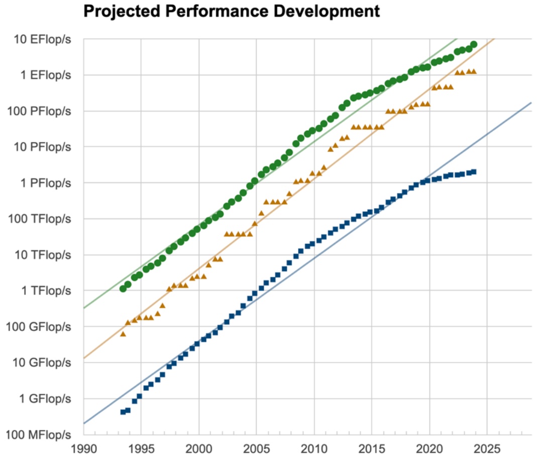
When we examine the world’s fastest supercomputers, they possess exaFLOPS and exaFLOPS of compute power – those are the green lines you see in the charts. That’s exactly what you’ll need to rely on if you’re attempting to train the biggest, most powerful language models today. Beyond the compute perspective, there’s also a crucial memory angle to consider, as these represent the two core resources and concerns for multi-machine parallelism. Many models are becoming quite large with billions and billions of parameters that simply won’t fit nicely into a single GPU, despite GPU memory growing over time. We must be very respectful of the memory constraints we face and understand how to split up memory and compute requirements across GPUs and machines.
🔴 Hardware Hierarchy and Communication Speed
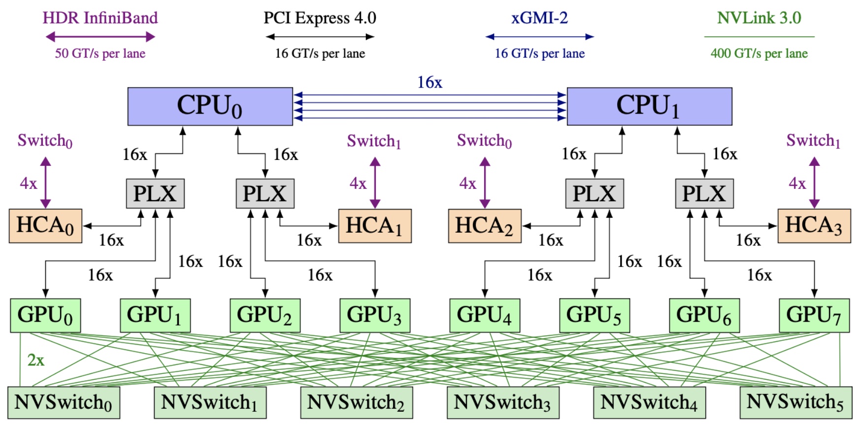
Critical insight: As you’ve probably noticed in the class cluster, GPUs don’t come in single units – a single machine will have multiple GPUs within the same physical rack, enabling intra-node parallelism via high-speed interconnects. In this architecture example, eight different GPUs are connected to various CPUs through fast interconnects, with an NVSwitch at the bottom providing very fast connections across these GPUs. However, when these GPUs need to communicate with GPUs on different machines, they must go through a networking switch using connections like HDR InfiniBand, which is significantly slower – about eight times slower per lane compared to NVLink connections. This hardware hierarchy has major implications for how we parallelize our models in practice, with very fast connections within a single machine but slower speeds when crossing machine boundaries.
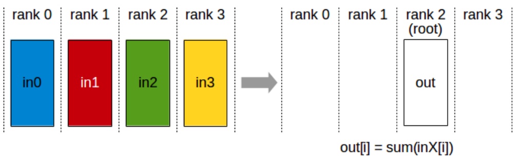
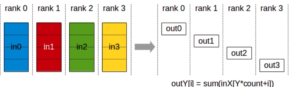
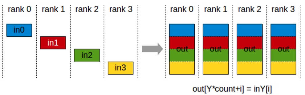
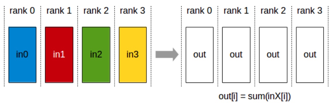
Let me provide a brief refresher on collective communication operations, particularly focusing on one important identity that you’ll need to understand the finer points of parallelization algorithm performance characteristics. All-reduce involves four machines or ranks, each with their own data, performing a reduction operation like summing all inputs, then copying the output to every machine – this costs roughly two times the total number of elements being all-reduced. Broadcast takes a single input from one rank and copies it to all remaining ranks, costing approximately one times the total number of outputs. Two other crucial operations are all-gather, where each rank takes a subcomponent of parameters and copies them to all other ranks, and reduce-scatter, which sums up rows and sends results to specific ranks – essentially a partial version of all-reduce. Understanding these collective operations is fundamental to grasping how different parallelization strategies leverage the networking hardware hierarchy we’ve discussed.
2. Communication Primitives and Hardware
Collective Communication Fundamentals
Before we dive into the hardware specifics and parallelization strategies, let me give you a very brief refresher on collective communication operations, because there’s one particular important identity or equivalence that you’ll need to know to really understand some of the finer points of the performance characteristics of parallelization algorithms. The first operation, which all of you probably have heard of, is all reduce. You have four machines, four ranks in this case, each one having its own piece of data. What you’d like to do is perform some sort of reduction operation – let’s say I want to sum all these inputs – and then I want the output to be copied over to every single machine. This is going to have roughly the cost of two times the total number of things that you’re all reducing.
You also have a broadcast operation, where I’m taking a single input from rank two and I’d like to copy it out to all the remaining ranks. This is going to have roughly on the order of one times the total number of outputs in terms of the communication cost. Then we’ve got reduction where we have different inputs that are summed up and sent only to one machine.
💡 All-Gather and Reduce-Scatter
The two that are quite important, even though these may not be quite as common, are all-gather and reduce-scatter. All-gather is an operation where I’m taking a single subcomponent of, let’s say, my parameters from rank zero and I’m copying it over to all the ranks. Same thing with rank one, two, three. So each of these are handling different parts of, let’s say, the parameters, and they’re copied over to the rest of the machines. So that’s copying what I have to everyone else.

The reduce-scatter operation is where I’m taking each of the rows, let’s say I’m summing them up, and then I’m sending the result only to rank zero. So this is a partial version of an all-reduce. All-gather and reduce-scatter are quite important because in some sense, they are the primitives by which many of the parallelization algorithms are going to be built. These operations will become especially relevant when we explore how to decompose more complex communication patterns.
The All-Reduce Identity
There’s one important identity I want to drill into you from the beginning, which has to do with all-reduce. If I have to all-reduce all my stuff – meaning I take everybody’s inputs, reduce them together, and then copy it to everybody else – there’s a very nice conceptual property where I can decompose the all-reduce into a reduce-scatter and an all-gather. First, I reduce the gradients and scatter them to everybody. So I’ll send the first portion of the summed-up gradients to rank zero, second portion to rank one, etc. Then I take what I have and copy it over to everyone else using all-gather. This decomposition costs roughly two times the size of the stuff that I’m all-reducing.
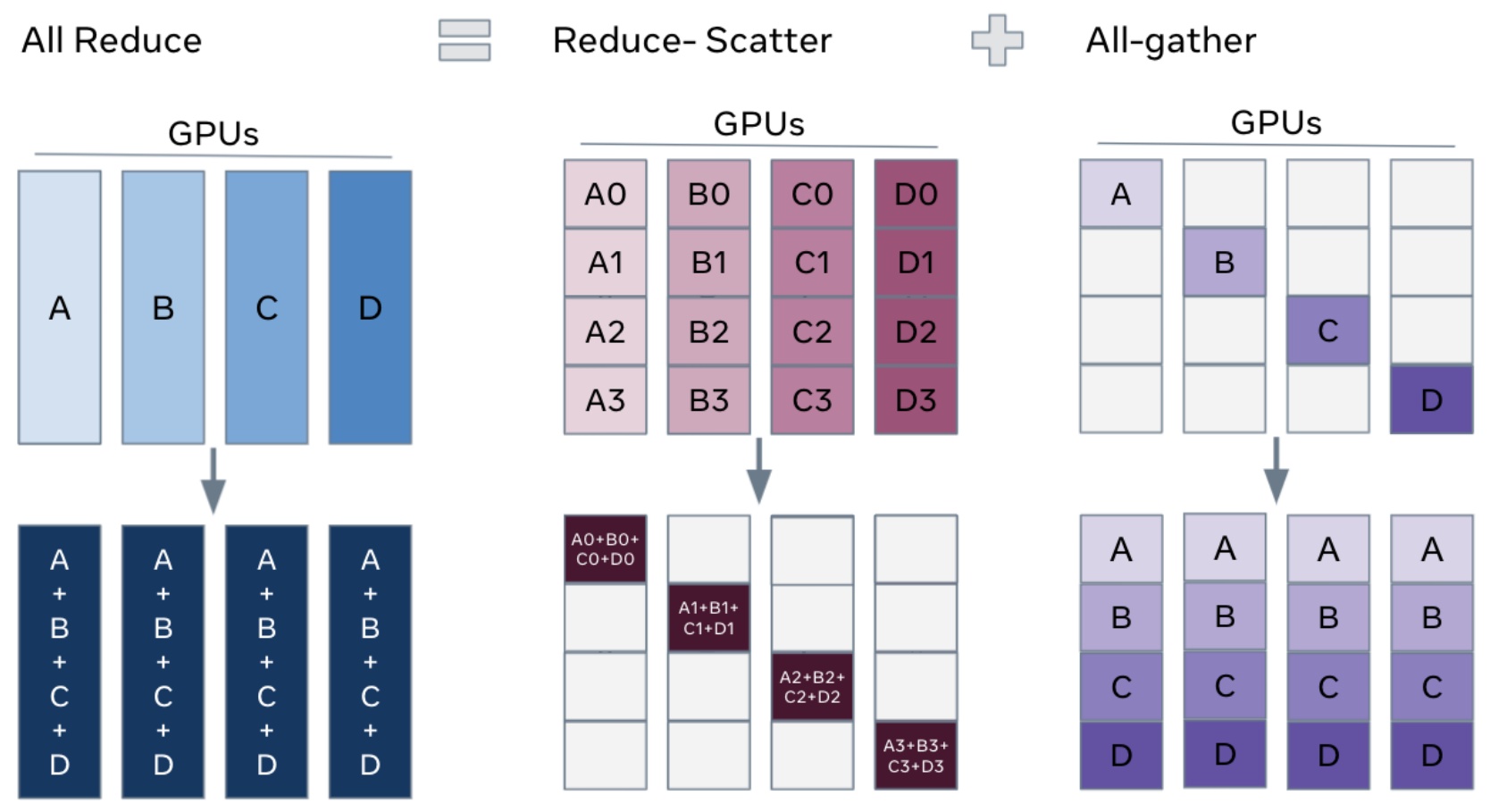
When you look at the cost, what’s a reduce-scatter? I’m reducing across everybody, and the output is going to scatter to everybody. The cost is going to be roughly \(1 \\times\) the size of my stuff. What’s the cost of an all-gather? Again, \(1 \\times\) the size of the stuff I’m all-gathering. And so \(1 + 1 = 2\), which is the same cost as directly doing an all-reduce. This property that reduce-scatter and all-gather is equivalent to all-reduce is something we’re going to use quite a bit when we talk about ZeRO, which is the kind of fundamental data-parallel optimization algorithm that we’re going to talk about in a second.
🔴 TPU vs GPU Architecture Differences
Hardware matters: GPUs and TPUs have fundamentally different networking architectures that impact parallelization strategies. GPUs typically use hierarchical InfiniBand switching, while TPUs employ a toroidal mesh topology. The TPU architecture supports better collective communication patterns because of its mesh structure, where you have nearest-neighbor connections that wrap around to form a torus. This means TPUs can be more efficient for operations that require heavy collective communications.
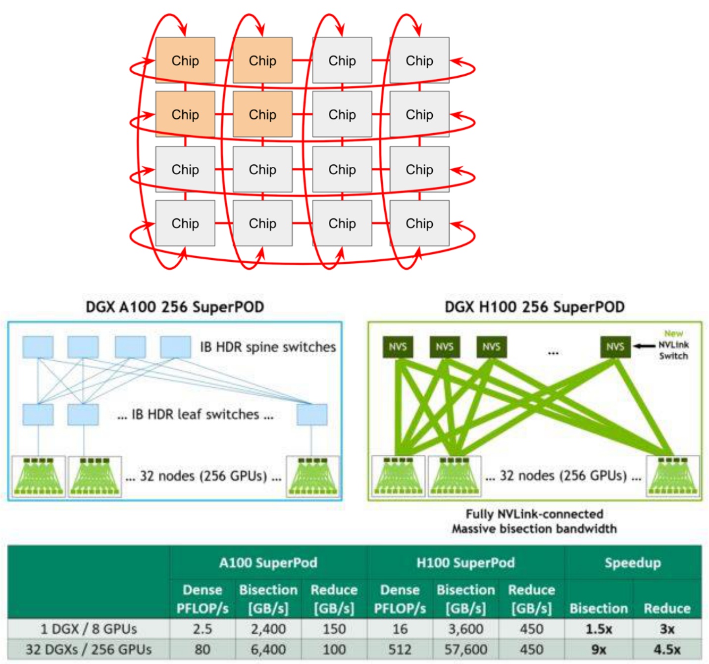
So if you’re optimizing purely for collective communications, it makes sense to think about things like TPU networking rather than GPU networking. This fundamental difference in networking architecture has important implications for how we design and implement distributed training algorithms across these different hardware platforms. With this hardware context in mind, let’s now explore how we can leverage these architectures for large-scale parallelism strategies.
3. Standard Data Parallelism Approaches
Three Fundamental Parallelization Strategies
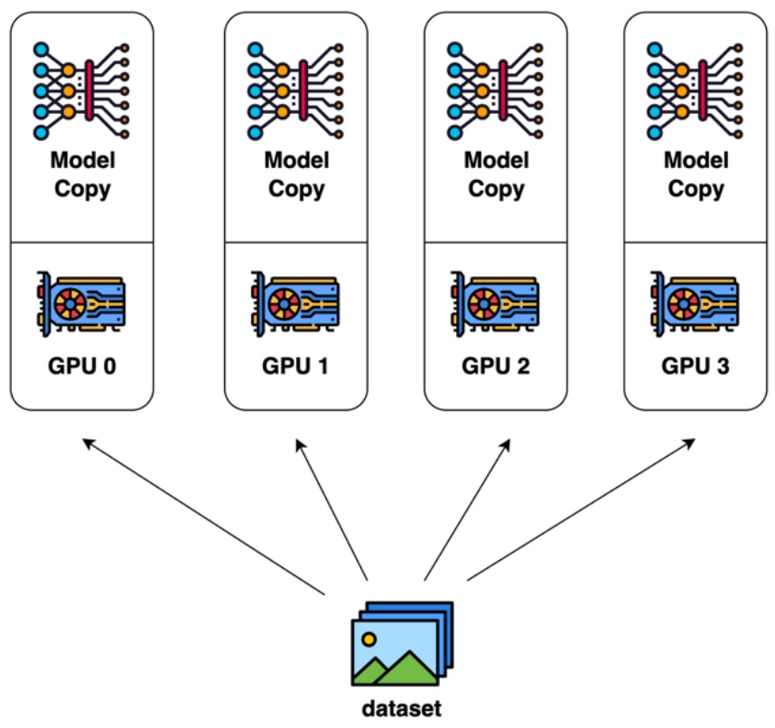
Now we’re getting to the exciting algorithmic meat of the lecture – understanding how to parallelize large language models effectively. When we think about scaling LLMs across multiple GPUs and machines, there are three fundamental parallelization strategies we need to master. The first approach is data parallelism, where we roughly copy the model parameters across different GPUs but split up our training batch. Each GPU or machine gets different slices of the batch to process, while maintaining identical copies of the model. This includes naive data parallel approaches as well as more sophisticated techniques like ZeRO levels 1-3 that optimize memory usage.
The second strategy is model parallelism, which becomes essential as our models grow larger. Rather than having all GPUs store all parts of the model, we need to cut up the model in clever ways so that different GPUs handle different components. This encompasses both pipeline parallelism, where we split the model across layers, and tensor parallelism, where we partition individual layers across devices. As models get bigger, having every GPU store the entire model becomes a significant memory bottleneck.
The final piece is activation parallelism, particularly sequence parallelism. While we don’t typically think much about activations in our day-to-day work because PyTorch handles them transparently, they become a major memory problem as models grow and sequence lengths increase. If you want to train really large models with substantial batch sizes, you must somehow manage the memory footprint of your activations by splitting them up strategically across devices.
When we combine all these parallelization strategies together, we have all the tools needed to scale both compute and memory gracefully across many machines. These are the core conceptual building blocks that allow us to train the massive language models we see today. Let’s start by diving into the most straightforward approach – data parallelism.
Naive Data Parallelism Implementation
The starting point of data parallelism is just sort of SGD, right? If we’re doing very naive batch-stochastic gradient descent, the formula for doing this looks like the equation shown here. I’m taking a batch size capital \(B\), and I’m going to sum up all those gradients and I’m going to update my parameters \(\\theta\).
$$\\theta_{t+1} = \\theta_t – \\eta \\sum_{i=1}^{B} \\nabla f(x_i)$$
Naive data parallelism is just saying, all right, take your batch size \(B\), split that up and send that to different machines. Each machine will compute some part of the sum, and then I will exchange all of my gradients together to synchronize. Before each gradient step, I will synchronize my gradients and then I will take a parameter update. This approach essentially splits the elements of a \(B\) sized batch across \(M\) machines and exchanges gradients to synchronize.
For compute scaling, data parallelism is pretty great. Each machine, each GPU is going to get \(B\) over \(m\) examples. And if my batch size is big enough, each GPU is going to get a pretty decent batch size, micro batch size, and it’s able to hopefully saturate its compute. What’s the communication overhead? Well, I’m going to have to transmit twice the number of my parameters every batch. Remember, an all-reduce is going to roughly be twice the amount of stuff that you’re all reducing in terms of communication costs. And so this is okay if the batch size is big – if my batch sizes are really big, I can mask the communication overhead of having to synchronize my gradients every now and then.
Memory scaling, I’m not touching this at all. Every GPU needs to replicate the number of parameters and needs to replicate the optimizer state. It’s pretty bad for memory scaling. So if we didn’t have to worry about memory at all, this is an okay strategy. But I think in practice memory is a problem, and this is where things get really challenging.
🔴 The Memory Crisis
Critical problem: Let’s dig deeper into why the memory challenges of naive data parallelism become particularly problematic when trying to scale training with larger batch sizes, which would otherwise make data parallelism more efficient. The memory situation is actually much worse than it initially appears – it’s quite terrible, really. While you might think you only need a simple copy of your model parameters, the reality is that you need to store multiple copies of your weights, consuming roughly 16 bytes of data per parameter depending on your training precision.
Where does this factor of eight memory overhead come from? Technically, your model parameters only need 2 bytes for FP/BF16 precision. However, you also need 2 bytes for FP/BF16 gradients since you’re computing gradients in the same precision. The real memory killer comes from your optimizer state, which creates a massive problem. You need 4 bytes for FP32 master weights – these are the accumulated values you’re updating in SGD. Additionally, Adam optimizer requires 4 or 2 bytes for first moment estimates since Adam keeps track of historical gradients, plus another 4 or 2 bytes for second moment estimates, which capture the variance of past gradients.
What originally looked manageable now appears quite grim. Most of your memory usage, at least in terms of parameter memory, is dominated by the optimizer states of your Adam optimizer rather than the core model parameters themselves. Your total memory consumption becomes a function of how many bytes your optimizer state requires, which generally exceeds even the combined parameter and gradient memory usage. For a concrete example, consider a 7.5B parameter model distributed over 64 accelerators – you’re consuming an enormous amount of memory, making this approach highly inefficient for large-scale training.
4. ZeRO Stage 1: Optimizer State Sharding
ZeRO Overview and Memory Solutions
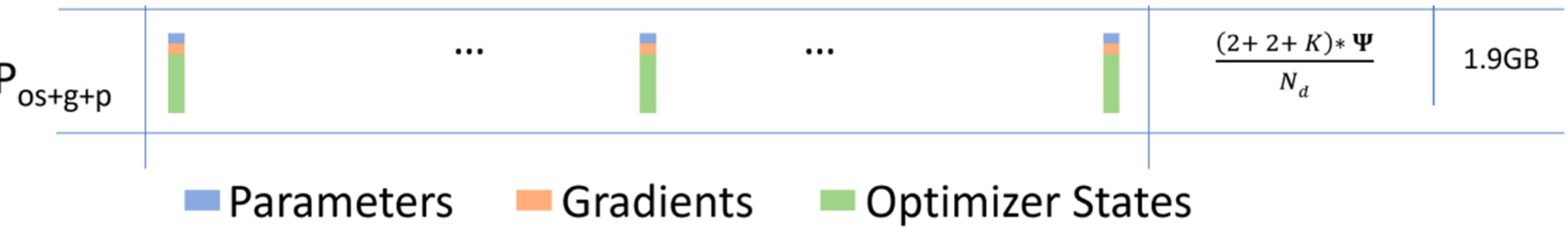
Let’s dive into one of the most impactful innovations in distributed training: ZeRO (Zero Redundancy Optimizer). When we examine memory scaling in distributed training, we encounter a fundamental problem: total memory scales linearly upwards with the number of GPUs, which is clearly suboptimal. However, looking at this challenge more carefully reveals some very simple yet powerful ideas. While parameters and gradients clearly need to be copied across devices for data parallel training, we might ask ourselves: do we really need all the optimizer states to be on every single machine?
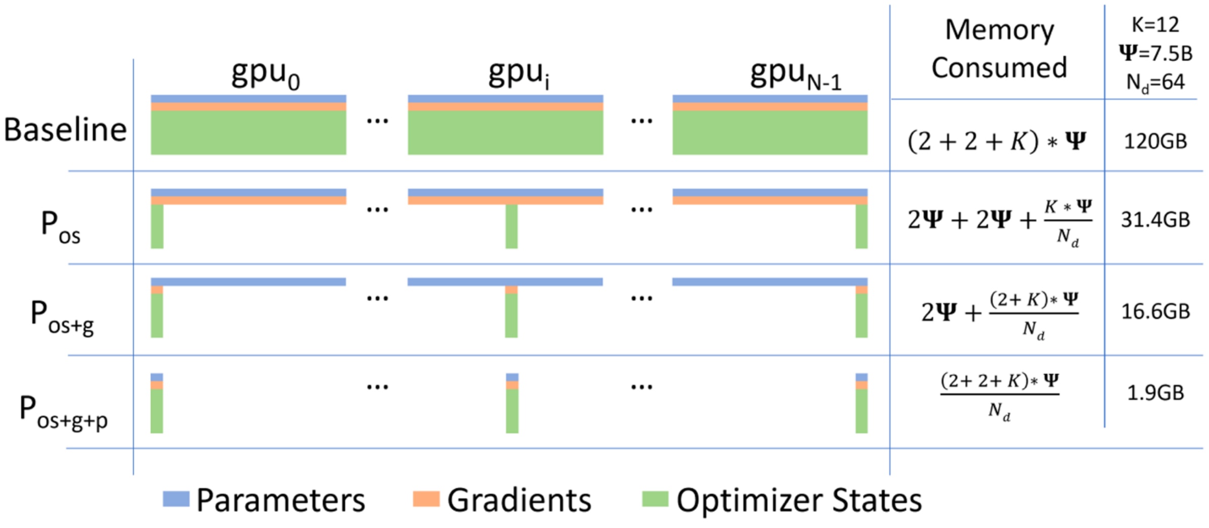
Once we ask that question, we can implement what’s called optimizer state sharding, which allows us to dramatically reduce memory usage from 120 gigabytes down to 31.4 gigabytes. But we don’t have to stop there – we can progressively shard the gradients to get down to 16.6 gigabytes, and then shard the parameters as well to reach an impressive 1.9 gigabytes of memory usage. This represents a fully sharded approach where all optimizer state, parameter, and gradient memory is distributed efficiently across devices.
You might wonder how this is even possible – after all, if GPU 0 has to be responsible for processing data point 1, it clearly needs to know about all the parameters to update them properly. How can it possibly shard the optimizer state? This is where ZeRO (Zero Redundancy Optimizer) comes in as a very clever solution. The core idea is to split up the expensive parts like optimizer states and use reduce-scatter equivalence for efficient communication. ZeRO demonstrates that even when doing data parallel training, you don’t actually need to copy everything onto every machine – you can be really clever about how you handle communications to avoid all this redundant memory usage. Let’s start by examining ZeRO Stage 1, which focuses specifically on optimizer state sharding.
ZeRO Stage 1 Implementation Details
Now that we understand the motivation behind ZeRO, let’s examine how Stage 1 actually works in practice. The core innovation of ZeRO Stage 1 lies in how we distribute the optimizer states across GPUs while maintaining computational efficiency. We split up the optimizer states – specifically the first and second moments used in optimizers like Adam – across all GPUs, but crucially, everyone still has access to the complete parameters and gradients. This design choice is fundamental because if I’m GPU 0 and I have the parameters and gradients for everything, that gives me enough information to compute the full gradient update. The limitation isn’t in computing the gradients – it’s that I can’t take that gradient and perform an optimizer step to update my parameters unless I have access to all the optimizer states.

Here’s how the distributed workflow operates in practice: GPU 0 computes the gradients for everything, but now it’s only responsible for updating the parameters for the specific shard that it owns. We distribute the work of parameter updates across all GPUs, then synchronize the parameters back. This approach is called ‘zero overhead’ because we maintain the same computational efficiency while dramatically reducing memory requirements. The key insight is that we can separate the computation of gradients from the application of optimizer updates, allowing us to distribute the memory-intensive optimizer states while keeping the computation distributed and efficient.
💡 The Four-Step Process
The implementation follows a precise four-step process. First, we split up the optimizer state (first and second moments) across GPUs while ensuring everyone has the parameters and gradients. Second, we perform a ReduceScatter operation on the gradients, which incurs a communication cost proportional to the number of parameters. This operation efficiently distributes and reduces the gradient information across all machines.
Third, each machine takes its sharded gradient and its sharded optimizer state to update the parameters it’s responsible for. Finally, we perform an AllGather operation to broadcast the updated parameters back to all machines, costing another one times the number of parameters in communication. This clever decomposition maintains the same total communication cost as naive data parallel while dramatically reducing memory requirements.
🔴 ZeRO Stage 1 vs Naive Comparison
The surprising magic: There’s a surprising bit of magic that happens with ZeRO stage 1 that makes it particularly elegant. In the naive approach, we were doing an all-reduce operation on all the gradients to ensure everyone’s gradients were synchronized, which cost us twice the number of parameters in communication overhead. However, if we’re clever about how we structure the updates, we can replace this with a reduce-scatter followed by an all-gather operation, with some computation happening in between these two steps.
This restructuring gives us the same communication cost as before, but now we’ve fully sharded the optimizer state across all GPUs in the model. The beauty of ZeRO stage 1 is that it’s essentially free in the bandwidth-limited regime while providing significant memory wins. The optimizer state memory per GPU is divided by the number of GPUs, which means you could theoretically track much more complicated optimizer states since that memory requirement scales inversely with the number of GPUs.
5. ZeRO Stage 2 and 3: Advanced Sharding
ZeRO Stage 2 Gradient Sharding
Building on ZeRO stage 1’s optimizer state sharding, ZeRO stage 2 takes the next logical step by also sharding gradients across machines. In addition to sharding optimizer states like in stage 1, we also keep the gradients (pink slices) sharded across the machines using the same rough tricks. However, there’s one additional complexity we need to handle: we can never instantiate a full gradient vector during the backwards pass, as this might cause us to go out of memory. Our maximum memory usage must be bounded by the combination of full parameters, sharded gradients, and sharded optimizer states.

The key insight is that we can’t compute the full gradient first and then do communication. Instead, as we compute gradients backwards through the computation graph, we need to handle them incrementally. Here’s how the process works: Step 1 – Everyone incrementally goes backward on the computation graph, and after computing a layer’s gradients, we immediately call a reduction operation to send this to the right worker. Since layers are sharded automatically to different GPUs, each layer belongs to a specific worker. Once gradients are no longer needed in the backward graph, we immediately free that memory.
After the gradient reduction phase, we move to Step 2 where each machine updates their parameters using their gradient and optimizer state. Since all machines now have their fully updated gradients and a full optimizer state for their share of the parameters, they can perform the parameter updates locally. Finally, in Step 3, we perform an all-gather operation to collect the parameters back together across all workers.
While this approach might look like it involves more communication because we’re doing reduction operations every layer, it’s actually only for a small amount of parameters since they’re sharded, so the total communication overhead remains the same. ZeRO stage 2 does have some additional overhead because we need to synchronize layer by layer and ensure gradients are properly sent to the right workers, but this overhead is pretty minimal. This sets us up perfectly for the most aggressive approach: ZeRO stage 3, which is more complicated but offers the greatest memory savings of all – essentially everything gets divided by the number of GPUs you have.
ZeRO Stage 3 (FSDP) Parameter Sharding
ZeRO Stage 3 represents the ultimate in memory efficiency, taking the sharding concept to its logical conclusion. It’s more complicated for sure, but it allows you the greatest win of all – essentially everything is divided by the number of GPUs that you have, giving you the maximum savings possible. If you’ve heard of FSDP, you’ve probably used that in some aspect of your life in the past. FSDP is exactly ZeRO Stage 3. We’re going to shard everything including the parameters, using the same incremental communication and computation ideas from ZeRO Stage 2. The key difference is that we send and request parameters on demand while stepping through the compute graph, both for the forward and backward passes.
💡 The On-Demand Parameter Fetching Strategy
The core trick in FSDP is prefetching parameters before they’re actually needed. Think of it like loading the next level in a video game before the player gets there. The process works like this: In the forward pass, I’ll start by doing an all-gather on parameters zero, which brings together all the shards from different machines. While the actual computation for layer zero is happening on the GPU, I can simultaneously request parameters one in the background. By the time computation zero finishes, parameters one should already be available, allowing me to immediately start computation one.
This clever overlapping of communication and computation is what makes FSDP practical. By the time computation zero is done, I can free weight zero since I no longer need it for the forward pass. The timeline shows how CPU operations coordinate with GPU computation and communication streams. You see that all gather 2 is already done before I need it, so there’s minimal waiting. The gaps are relatively small, and we’re able to do a lot of loads before the compute actually needs to happen.
That’s the entirety of the forward pass. You see that the gaps are relatively small here, and we were able to do a lot of loads before the compute needed to happen. By doing this very clever thing of queuing the requests for weights before you actually need them, you can avoid a lot of the overhead associated with communication. At this point, I’m done with the forward pass, I can free weight number 2, and I start on the backward pass. You see that all gather 2 for the backward pass is already done, so I can start on backward 2. The higher overhead happens in the backward pass because I need to do reduce-scatters and all-gathers. Hopefully you see this picture and say, wow, it’s kind of surprising that even though we’re doing this crazy sharding where we fully shard the parameters, gradients, and optimizer states, the actual bubbles that we see are not horrendous. The communication is almost being fully utilized, and the computation isn’t stalling for very long, so we’re actually making pretty efficient use of the resources that we do have. This brings us to the broader question of how these communication costs compare across different ZeRO stages.
ZeRO Communication Costs and Benefits
Now that we’ve seen how FSDP achieves its efficiency through clever scheduling, let’s step back and compare the communication costs across all ZeRO stages. ZeRO represents the modern approach to distributed data parallel training, offering different stages with varying communication costs and benefits. ZeRO stage 1 operates at \(2 \\times \\#\) param communication cost – essentially free since it maintains the same communication pattern as naive data parallel while providing sharded optimizer states. You might as well always use it! ZeRO stage 2 also runs at \(2 \\times \\#\) param, making it almost free as well, though there is some overhead from the incremental freeing of gradients during the backward pass.
ZeRO stage 3 becomes more involved, requiring \(3 \\times \\#\) param in communication costs – about 1.5x the communication overhead. While this represents three times the number of parameter communications, it’s actually not so bad in practice. The key insight is that if you cleverly mask your communication patterns, the performance remains quite good. The communication pattern involves 2 all-gather operations (\(\\#\) param each) and 1 reduce-scatter (\(\\#\) param), but the latency can be effectively hidden with proper implementation.
One of the major advantages of data parallel approaches like ZeRO is their conceptual simplicity and architecture-agnostic nature. People successfully use data parallel training even with fairly slow networking links because the communication patterns are well-understood and predictable. The approach doesn’t require deep knowledge of the specific neural network architecture – whether you’re training a transformer or any other model, the parallelization strategy remains abstracted from the implementation details.
This architecture-agnostic property explains why frameworks like FSDP (Fully Sharded Data Parallel) have become so popular in the community. It’s remarkably easy to write a wrapper that parallelizes arbitrary neural networks without requiring deep introspection into what the architecture is actually doing under the hood. This simplicity, combined with the reasonable communication costs across all ZeRO stages, makes it an attractive choice for distributed training at scale. However, as we’ll see next, there are other parallelization strategies that can offer different trade-offs, particularly when we’re willing to think more carefully about the specific structure of our neural networks.
6. ZeRO Practical Applications and Limitations
Memory Fitting Analysis
Now let’s examine the practical impact of ZeRO optimizations by analyzing memory fitting capabilities. When you look at what’s the maximum size of the model that I can fit on an 8 times 180 gig node, the results are quite dramatic. For baseline configurations, you might end up with the ability to fit barely a 6 billion parameter model. However, if I use ZeRO stage 3, I’m able to fit something like a 50 billion parameter model – that’s a dramatic improvement in capacity.
There are big savings in my ability to fit larger and larger models by doing things like FSDP to cleverly save on memory and avoid running out of memory on my GPUs. You could call this a kind of parallelism, but the whole point of model parallelism is fundamentally different – it’s to make sure that the parameters just live entirely in one machine.
With model parallelism, we’re not going to try to ship parameters across machines in various ways. Only the activations are going to get shipped across different nodes. This creates a very different focus in the model parallelism discussion – the emphasis there will be on communicating activations rather than communicating parameters, which is a key distinction from the memory optimization approaches we’ve been examining. However, before we dive into model parallelism, we need to understand the fundamental limitations that drive us toward these alternative approaches.
🔴 Remaining Data Parallel Challenges
Critical limitation: Despite the impressive gains we’ve seen with ZeRO, data parallel training still faces fundamental constraints that limit its scalability. The most critical of these is that batch size emerges as a finite resource that fundamentally limits scalability. The key constraint is that you can’t parallelize beyond your batch size – with data parallel, the number of machines must be less than the batch size since you can have at most one example per machine, and you certainly can’t have fractional examples. This creates a hard ceiling on parallelization that becomes particularly problematic when communication overhead increases as you approach this limit.
The situation becomes even more complex due to diminishing returns from increasing batch sizes. As you may have experienced in assignment one when experimenting with different batch sizes, cranking up the batch size past a certain point leads to fairly rapid diminishing returns in optimization rates. OpenAI’s research on critical batch sizes provides valuable insight here – they argue that beyond a certain threshold, you see very rapid diminishing returns in how much each example contributes to your optimization ability. The intuition is straightforward: below a certain point, you have significant gradient noise, and reducing that variance is extremely valuable. However, at a certain point, you become fundamentally limited by the number of gradient steps you’re taking rather than variance reduction.
This means that data parallel alone simply won’t get you to arbitrarily large parallelism. You essentially have a fixed maximum batch size that becomes a resource you need to spend wisely across different types of parallelism. The remaining issues with current data parallel approaches are significant: ZeRO stages one and two don’t allow you to scale memory effectively, and while ZeRO stage three is nice in principle, it can be slow. More importantly, it doesn’t reduce activation memory, which is a crucial limitation.
What we really want is to cut up our models entirely and make them live totally separately, because then the activation memory would also be reduced. This need for better ways to split up models so we can fit these really big models across multiple GPUs naturally brings us to model parallelism – a fundamentally different approach where parameters are distributed across separate machines rather than replicated.
7. Pipeline Parallelism
Introduction to Model Parallelism
When we want to scale up memory without changing batch size, we need an alternative parallelization axis that doesn’t require large batch sizes. Model parallelism offers this solution by splitting parameters across GPUs, similar to ZeRO-3, but with a key difference: instead of communicating parameters, we pass activations around. This is often advantageous because activations can be much smaller than parameters, leading to more efficient communication patterns.
There are two main types of model parallelism we’ll explore, each corresponding to different ways of cutting up the model. First is pipeline parallelism, which is conceptually the most obvious way to partition a neural network – it’s straightforward to understand but can be quite horrible to implement in practice. Second is tensor parallelism (along with sequence parallelism), which might be less conceptually obvious at first but is honestly much nicer to implement and more commonly used in real-world applications.
The fundamental trade-off here is between implementation complexity and conceptual clarity. While pipeline parallelism follows the natural flow of data through network layers, making it intuitive to grasp, tensor parallelism’s more sophisticated approach to distributing computation often results in cleaner, more maintainable code and better performance characteristics in practice. Let’s start by examining the most intuitive approach – distributing layers across GPUs.
🔴 The Layer-wise Parallelism Problem
Critical inefficiency: The most natural starting point for pipeline parallelism is to cut the network at layer boundaries and distribute different layers across multiple GPUs. In layer-wise parallel processing, each GPU handles a subset of the layers, with activations being passed forward from one GPU to the next during the forward pass, and gradients being passed backward during backpropagation. This seems like an intuitive way to leverage multiple GPUs, but as we’ll see, this approach has some serious limitations.
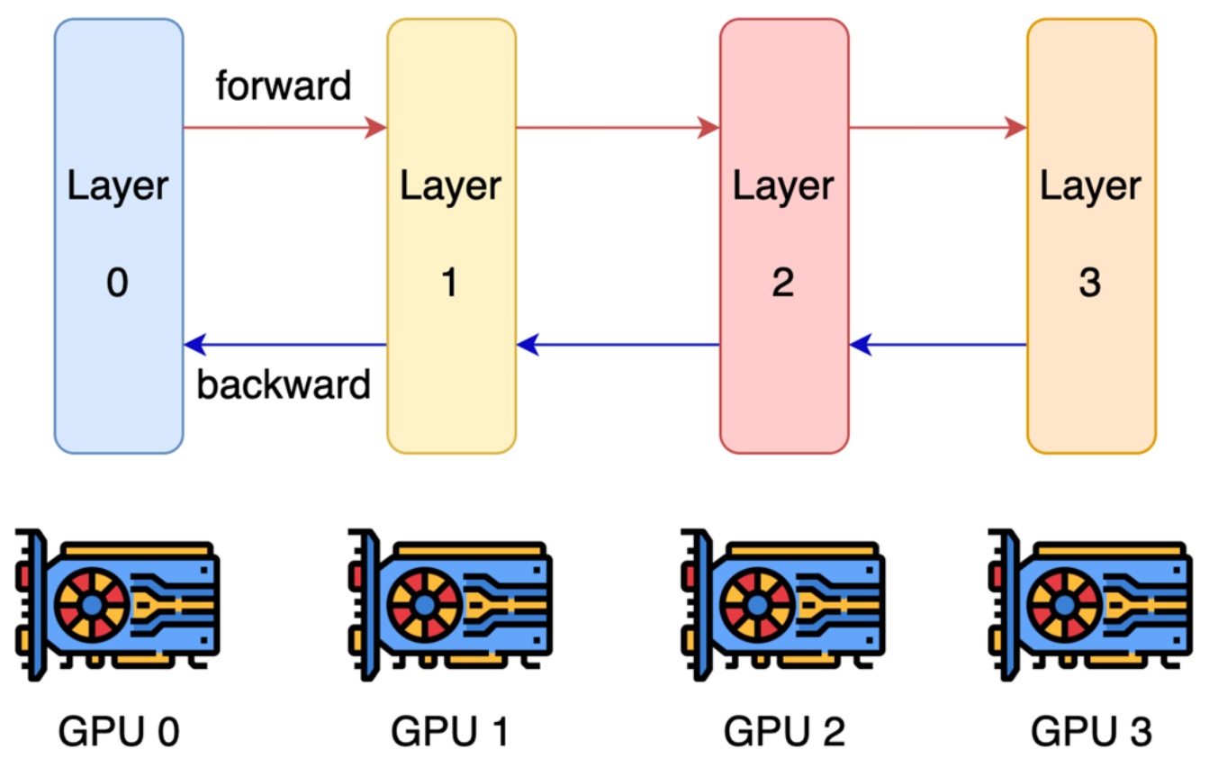
The fundamental problem with this naive layer-wise parallelism becomes apparent when you examine GPU utilization over time. Most of your GPUs end up being idle most of the time, which is terrible for computational efficiency. When processing a single example through the network, GPU 0 computes the first layer, then passes activations to GPU 1, which wakes up to compute the second layer, and so on. This creates what’s known as a ‘bubble’ – a massive overhead period where GPUs are doing absolutely nothing while waiting for their turn.
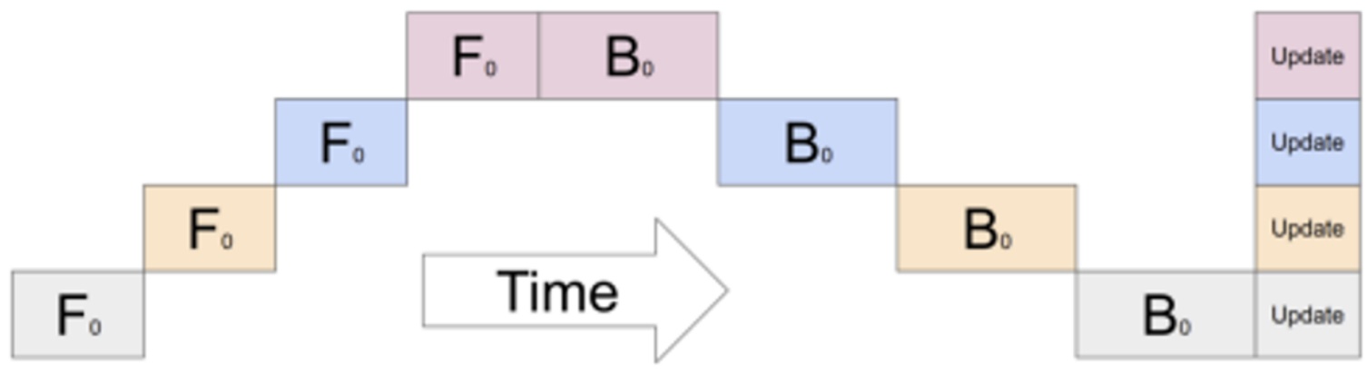
With \(n\) gpus, each gpu is active \(\\frac{1}{n}\) of the time.
This utilization pattern represents perhaps the worst possible parallelism scenario. Even though you’ve added four GPUs to your system, you’re only getting the throughput equivalent to a single GPU because each GPU is active only \(\\frac{1}{n}\) of the time, where \(n\) is the number of GPUs. The sequential nature of layer-by-layer processing means that adding more GPUs doesn’t improve performance – it just creates more idle time.
Fortunately, there are more clever approaches to address this inefficiency. The key insight is that we can overlap computations by processing multiple examples simultaneously across the pipeline stages, which brings us to proper pipeline parallel solutions.
Pipeline Parallel Solutions
The solution to the layer-wise parallelism problem lies in processing sequences of micro-batches across GPUs to achieve better efficiency. The key insight is that each machine handles a subset of examples – say four examples per micro-batch – and can immediately send activations to the next GPU as soon as it finishes processing the first data point. This creates an overlapping pattern where the second GPU starts working while the first GPU continues processing subsequent data points, effectively overlapping communication and computation to reduce the dreaded pipeline bubble.
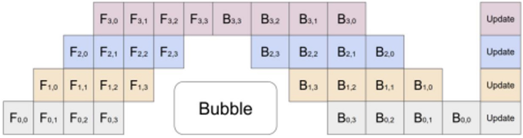
One popular scheduling strategy is called GPipe or 1F1B (one-forward-one-backward), which is quite elegant in its simplicity. After doing a forward pass through layer 0, you immediately start the backward pass for that same layer while simultaneously beginning the forward pass for the next example. This interleaving creates a much better utilization pattern. The remaining bubble size in the pipeline becomes proportional to the number of pipeline stages divided by the number of micro-batches. This means that if you have lots of micro-batches, you can minimize the bubble overhead significantly.
💡 Advanced Pipeline Optimization: Zero Bubble
Of course, you can implement different kinds of pipeline strategies beyond these standard patterns. Instead of having basic scheduling approaches, you can cut things up into finer pieces where you’re assigning different sub-layers to different devices and doing different computations at different parts. This allows you to interleave the pipeline much more effectively.
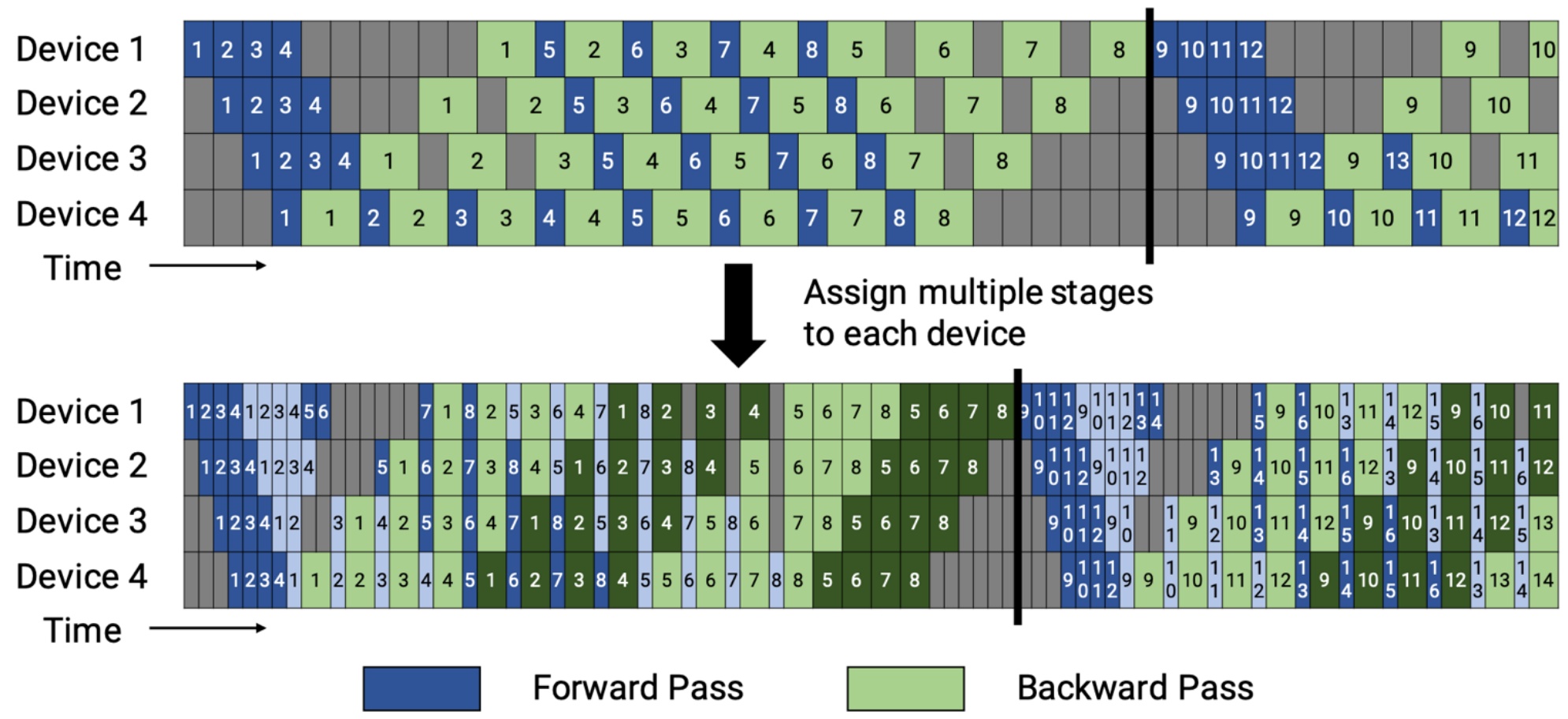
An advanced version of this that’s very, very clever is zero bubble pipelining, which DeepSeek calls dual pipe, but the core trick is the same. The key insight is that when you’re doing the backwards pass to compute gradients, you can split this up into two different components. The first part involves backpropagating the activations – computing the derivative with respect to the activations as you go down the residual connections. The second part involves computing the gradient itself for parameter updates. To give you a concrete example, consider a single MLP where you multiply by a weight \(W\), apply a non-linearity, and output the result. In the backwards pass, you have the derivative with respect to the loss coming in, and you compute how that changes the inputs \(x\) to your MLP – these are the derivatives with respect to the activations. Then you use these to compute the gradients needed to update your weights \(W\).
The crucial realization is that computing the gradients for the weights can be done whenever you want – there’s no serial dependence on this computation, so you can reschedule it to any part of the computation graph. What you can do is use standard pipeline parallel for the parts that are serially dependent, but any time you need to do computations just for updating parameters, you can reschedule them wherever there’s available capacity. Starting with a nice 1F1B (one-forward-one-backward) pipeline that reduces bubble size, you can separate the \(B\) computation (backwards part) from the \(W\) computation (weight gradients), and then do the weight computations where you originally had bubbles. Those white idle utilization periods can now be filled with these \(W\) computations, giving you much better GPU utilization by thinking carefully about what the serial dependencies actually are.
🔴 Implementation Complexity Warning
Reality check: To be completely clear, this approach is horrendously complicated to implement. If you actually want to implement pipeline parallel this way, you’ll need to intervene in how your auto-diff calculates things and maintain queues that track where computations go. I heard a funny but sobering anecdote recently from someone at a frontier lab: they said there were originally two people in their group who understood how pipeline parallel worked in their infrastructure, and one person left. So now there’s a single load-bearing person in their entire training infrastructure! Pipeline parallel is infrastructurally very, very complicated – it looks simple in these diagrams, but if you’re interested in trying to implement it, it gets pretty hairy pretty fast.
8. Tensor Parallelism
Tensor Parallel Implementation
Now let’s explore tensor parallelism, the other major form of model parallelism that’s much simpler and more widely adopted than pipeline parallelism. This approach is cleanly utilized by many frameworks, and people training really big models rely very heavily or primarily on this kind of model parallelism. The key insight is that most of what we do in big models is matrix multiplies – most of the computation and most of the parameters are matrices. If we can parallelize just the matrix multiplies, that would be pretty effective.
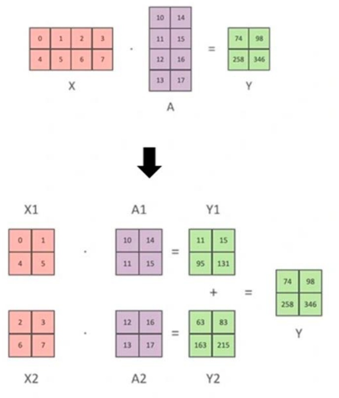
Tensor parallel is this idea that we can take a big matrix multiply and split it up into a set of sub-matrices that can be multiplied. If I have a matrix multiply \(x \\times a = y\), I can cut up \(a\) into halves, and I can also cut up \(x\) into halves. I can compute the sub-matrices, sum them up, and get my answer at the end. Conceptually, pipeline parallel is cutting along the depth dimension (the layers), while tensor parallel is cutting along the width dimension of your matrix multiplies. We decompose into sub-matrices and then do partial sums.
💡 MLP Example Implementation
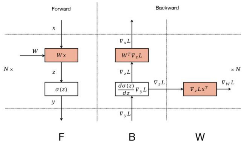
Here’s how it works in practice with an MLP: each GPU handles a different sub-matrix of a big MLP matrix multiply, and we use collective communications to synchronize activations as needed. Let’s say I want to compute \(y = \\text{GeLU}(x \\times a)\) followed by \(z = \\text{Dropout}(y \\times b)\). I split my parameter matrices \(a\) into \(a_1\) and \(a_2\), and \(b\) into \(b_1\) and \(b_2\). In the forward pass, I take my inputs \(x\) and copy them to both GPUs. Each GPU operates with \(a_1\) and \(a_2\) respectively, giving activations \(y_1\) and \(y_2\). These go through \(b_1\) and \(b_2\), and then I do an all-reduce to sum them up and get the final answer \(z\).
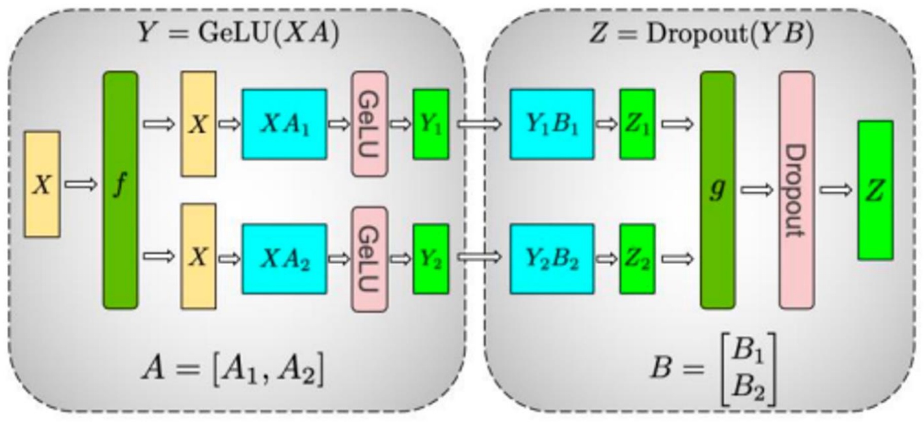
The backward pass works in reverse. As gradients flow backwards, the operations \(f\) and \(g\) serve as synchronization barriers at different points. In the forward pass, \(f\) is the identity and \(g\) is an all-reduce. In the backward pass, \(f\) is an all-reduce and \(g\) is the identity. The gradients get copied on both sides, and I do the backwards operation all the way through. When I get to the all-reduce point, I have two derivatives coming in from both paths that get summed back up. This creates a very clean way to parallelize any matrix multiply by simply cutting up the matrices and distributing them across different devices. However, this simplicity comes with important practical considerations about when to use this approach.
🔴 When to Use Tensor Parallelism
Hardware constraint: While tensor parallelism offers elegant simplicity, it’s actually somewhat expensive in practice. We have a synchronization barrier that lives per layer, and it needs to communicate an activation – sort of like the residual activation worth of stuff – twice in a forward backward pass. So tensor parallelism, this very simple idea, is going to require very high-speed interconnects. There’s a very simple rule of thumb to remember: tensor parallelism is applied within a single node.
A single box of, let’s say, NVIDIA GPUs is going to ship with eight different GPUs that live in that same box. And as I showed you at the beginning of lecture today, they’re very, very high-speed connected. So those eight GPUs can talk to each other very quickly, and it makes sense to use something like tensor parallelism that’s very bandwidth-hungry between those eight devices. What we will typically see is that tensor parallelism is applied up to 8 GPUs, where the GPUs live in the same machine, because that gives you the least drop in performance.
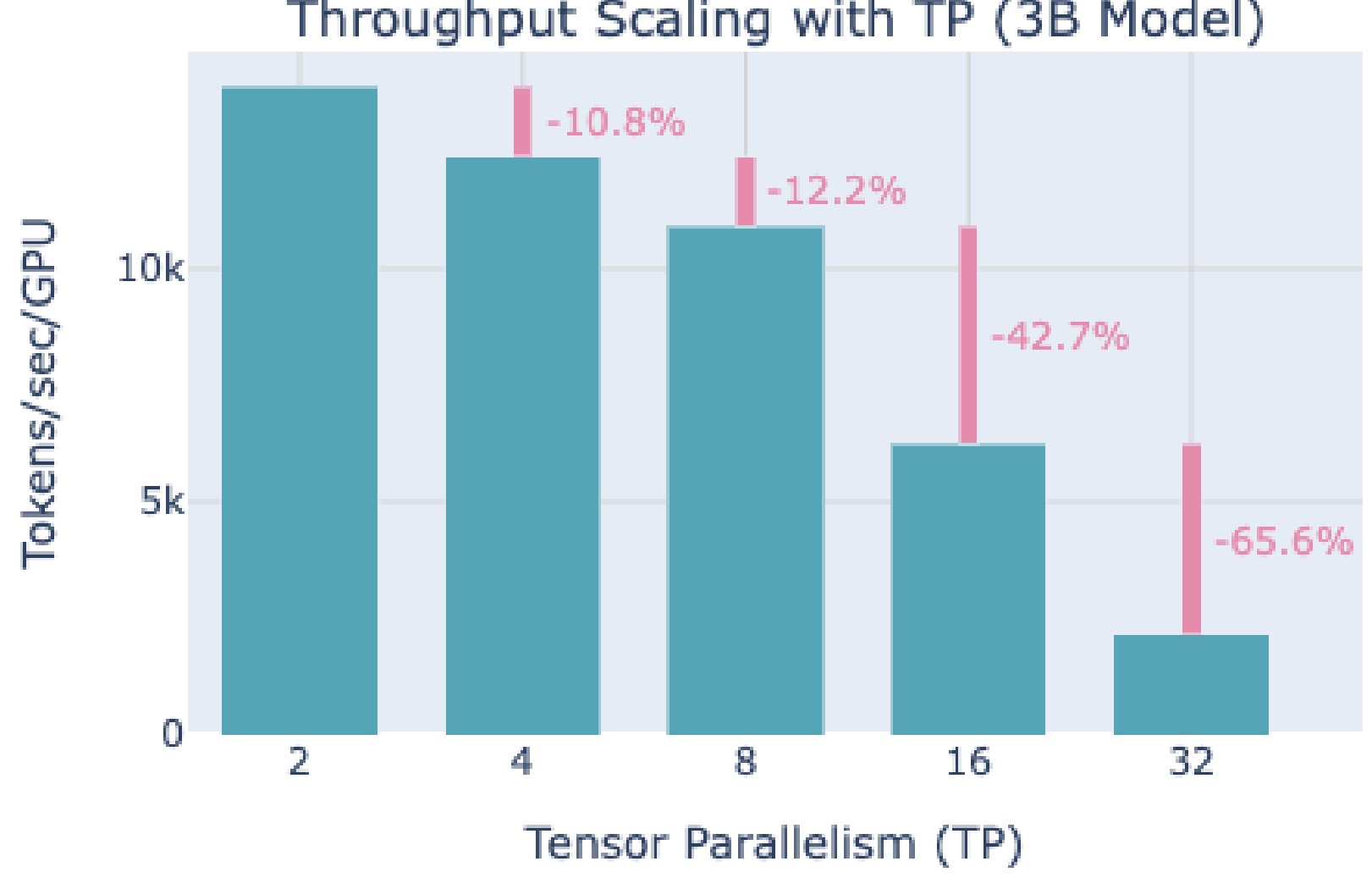
This is an example from Hugging Face’s parallelization tutorial showing you the throughput decreases of different levels of tensor parallelism. You see that there are hits – 10% and 12% hits to throughput as you do tensor parallelism. But up until 8 devices, well, maybe this is manageable. This is kind of the price you pay for just being able to parallelize more nicely. But then you go to 16 devices and you get this kind of astounding 42% drop in performance. You go to 32 and you see another 65% drop in throughput.
So you see, hopefully, visually here that you really want to stop at 8 for tensor parallelism. That’s really the sweet spot because of the kinds of hardware interconnects you can get your hands on. On GPUs, tensor parallelism works best within a node – up to 8 GPUs – due to those high-speed interconnects that allow the devices to communicate efficiently without significant performance degradation. This performance characteristic leads us to an important comparison with pipeline parallelism.
Tensor vs Pipeline Parallel Trade-offs
Now that we understand both approaches, let’s compare their trade-offs directly. When comparing tensor parallel to pipeline parallel, several key advantages emerge. Unlike pipeline parallel, tensor parallel doesn’t suffer from the bubble problem that plagued the previous approach. There’s no need to consume larger batch sizes just to reduce inefficient bubbles, which is a significant benefit. The implementation complexity is also relatively low – you primarily need to identify where the big matrix multiplies occur and determine how to split them across different devices. The forward and backward operations remain fundamentally the same, making tensor parallel much more straightforward to implement compared to complex approaches like zero overhead or dual pipe pipeline parallel.
However, tensor parallel comes with a major drawback: substantially larger communication overhead compared to pipeline parallel. While pipeline parallel requires only \(bsh\) point-to-point communication per microbatch (where \(b\) is batch size, \(s\) is sequence length, and \(h\) is the hidden dimension), tensor parallel demands \(8bsh \\left(\\frac{n_{devices}-1}{n_{devices}}\\right)\) communication per layer using all-reduce operations. This represents roughly eight times more communication overhead per layer, which can become a significant bottleneck depending on your hardware setup.
The rule of thumb for choosing tensor parallel is straightforward: use it when you have low-latency, high-bandwidth interconnects. In practice, you’ll typically see 2 to 16 devices used for tensor parallel, depending on the specific machine configurations. Interestingly, these approaches aren’t mutually exclusive – they’re often used simultaneously in large-scale training runs. The typical pattern involves using tensor parallel within a single machine, then applying a combination of data and pipeline parallel across multiple machines. Pipeline parallel is primarily employed when models simply won’t fit in memory, whereas if your entire model can fit, you’d typically just use data parallel plus tensor parallel, or potentially just data parallel alone.
9. Memory Management and Activation Optimization
Dynamic Memory Challenges
As we dive deeper into parallelization strategies, memory management has become a critical aspect when training large models, and one of the most significant yet often overlooked components is activation memory. When we examine the standard forward-backward pass, we see that memory usage is highly dynamic throughout the training process. While parameters remain static during training, the memory landscape changes dramatically across iterations. In iteration 0, there’s no optimizer state yet, so that portion of memory usage is absent. However, as we progress through the forward pass, activation memory grows continuously as we accumulate all the intermediate activations needed for backpropagation.
The memory dynamics become particularly interesting during the backward pass. As we start backpropagation, activation memory begins to decrease because we free activations as we consume them for gradient computation. Simultaneously, gradient memory usage increases as we accumulate gradients. The peak memory usage occurs partway through the backward pass, where we haven’t yet freed all activations but are still building up gradients. This pattern repeats consistently across iterations, highlighting a fundamental challenge in memory management.
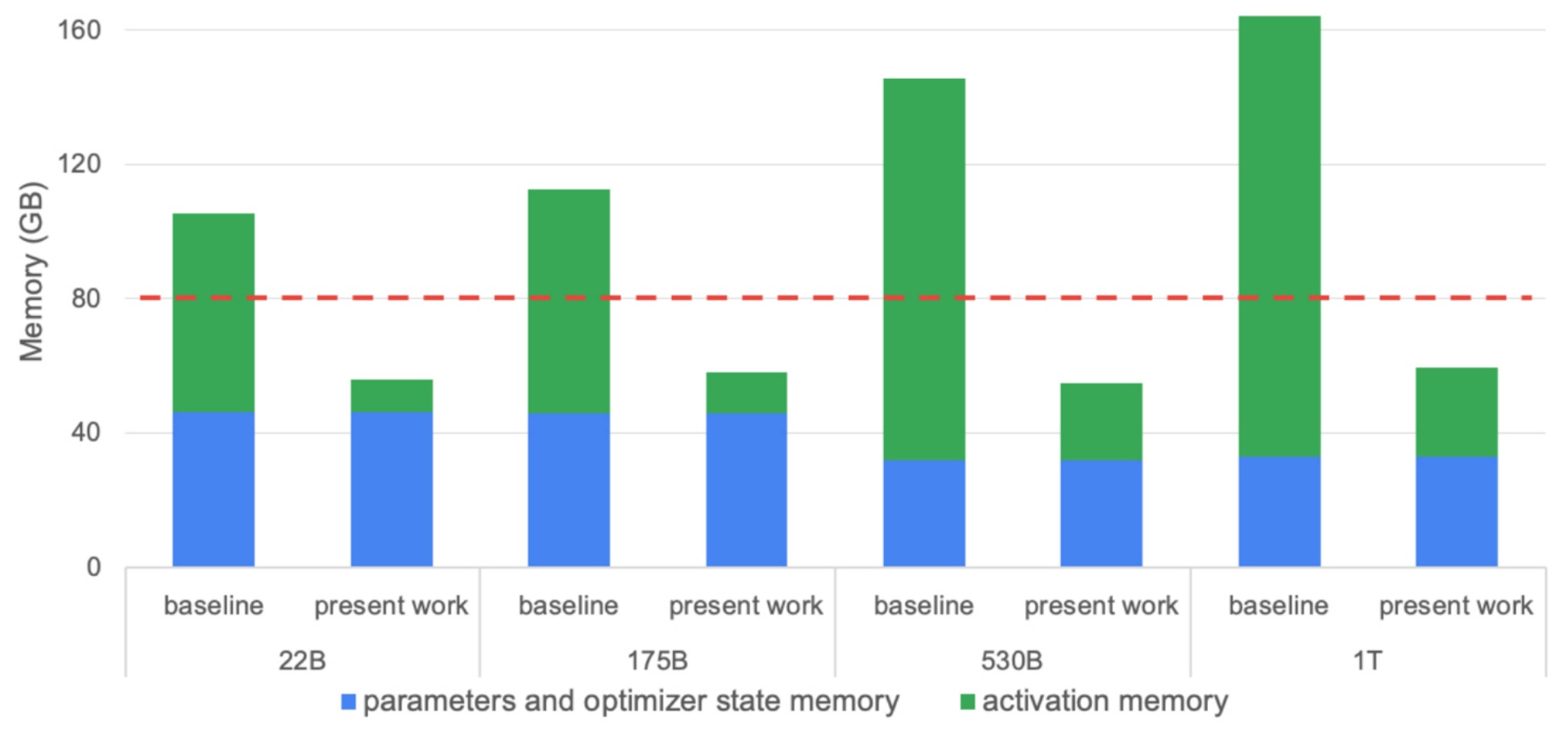
While tensor parallelism and pipeline parallelism can linearly reduce most memory components like parameters and optimizer states, they struggle with activation memory reduction. This limitation becomes increasingly problematic as models grow larger. As demonstrated in research from Nvidia, when we scale models from smaller to larger sizes, parameter and optimizer state memory can remain constant through aggressive parallelization, but activation memory continues to grow per device. This growth occurs because certain parts of activation memory don’t parallelize cleanly, meaning that regardless of the number of devices available, we can’t eliminate the per-device growth of activation memory.
💡 Activation Memory Formula
To understand activation memory requirements more precisely, we can calculate the memory needed per layer using a specific formula. The activation memory per layer follows a clear pattern with two distinct components:
$$\\text{Activations memory per layer} = sbh \\left(34 + 5\\frac{as}{h}\\right)$$
This formula reveals the underlying structure of memory requirements. The left term, \(sbh \\times 34\), represents memory needed for MLP and other pointwise operations, which depends on the size of the residual stream \(h\). The right term, \(5\\frac{as}{h}\), comes from quadratic attention terms including dropout. When we multiply this out, we get \(as^2b\) (since \(h\) cancels), representing the memory required for softmax and other quadratic attention operations. However, with techniques like Flash Attention and recomputation, we can drastically reduce this second term, making it possible to keep activation memory low even for the largest models. This understanding of memory components leads us naturally to examine how tensor parallelism affects these calculations.
Activation Memory under Tensor Parallelism
Building on our understanding of activation memory components, when implementing tensor parallelism in transformer models, we apply it everywhere possible – in the MLPs, in the key-query computations, and throughout the attention mechanisms. This comprehensive approach yields significant improvements in memory efficiency, but the results reveal an interesting limitation that’s worth examining closely.
$$\\text{Activations memory per layer} = sbh \\left( 10 + \\frac{24}{t} + 5 \\frac{as}{ht} \\right)$$
Looking at the activation memory per layer divided by \(T\) (the number of devices we’re tensor paralleling over), we can see the approach is quite effective but not perfect. If we’re dividing by eight devices, ideally we would see all activation memory reduced by a factor of eight. However, there’s a persistent straggler term – \(SBH \\times 10\) – that stubbornly refuses to be reduced down proportionally.
This remaining term represents the non-GEMM components of our computation: layer normalization, dropout operations, and the inputs to both attention and MLP layers. Unfortunately, these components continue to grow with model size and cannot be parallelized as elegantly as the matrix operations. This limitation becomes increasingly significant as we scale up our models, representing a fundamental challenge in achieving perfect parallelization efficiency. However, there’s a solution to this remaining bottleneck that involves parallelizing across the sequence dimension.
Sequence Parallel for Linear Memory Scaling
To address the stubborn non-GEMM components we just discussed, the final piece of the sequence parallelism puzzle involves handling the simple pointwise operations that we haven’t parallelized yet. These operations, like layer normalization and dropout, can be split up in a straightforward manner because they don’t interact across different positions in the sequence. For instance, layer norms at different sequence positions are completely independent of each other. So if we have a 1024-long sequence, we can cut it up and have each device handle a different part of that layer norm or dropout operation. These pointwise operations can now be completely split across the sequence dimension.
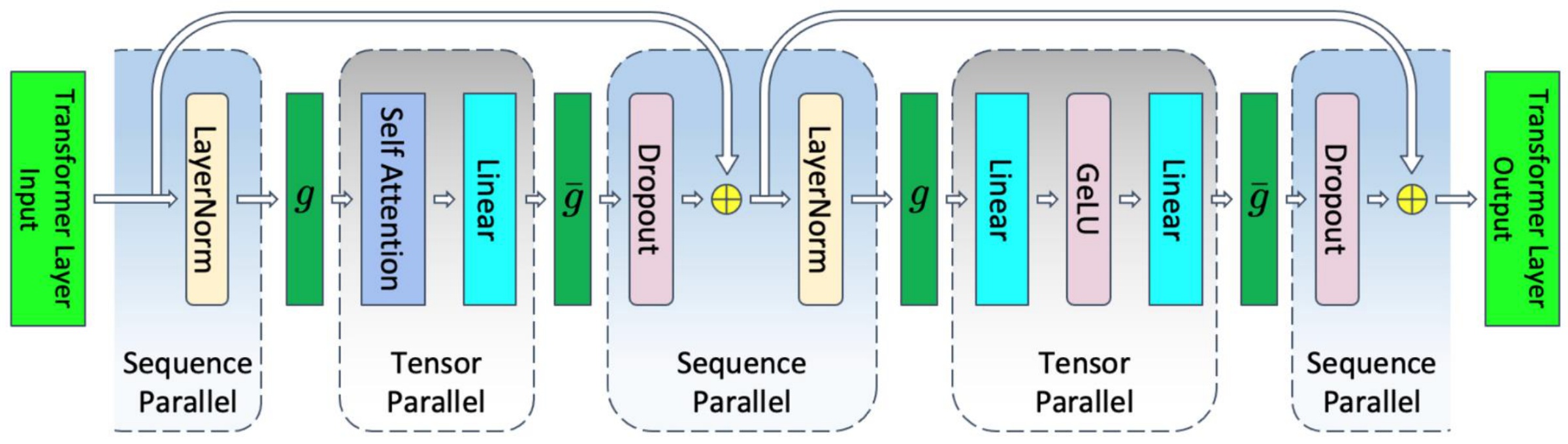
Because we’re now cutting things up across the sequence dimension, we need synchronization to ensure the parallel computations can be aggregated back together. In the forward pass, the \(g\) operations are all-gathers, and the \(\\bar{g}\) operations are reduce-scatters. In the backward pass, these two are reversed – there’s a sort of duality here between the forward and backward passes. For layer norm, we’ve scattered things around, so we need to gather them back together to do our standard computation. Then when we get to dropout, we want to scatter them back out into the parallel components we have. The backward pass does this in reverse.
This is really a very simple idea – we’re just parallelizing the very last components that we failed to parallelize before. Now we can put all these different pieces together and see the complete picture. We started with no parallelism at all, then applied tensor parallelism which allows us to divide everything that’s not a pointwise operation by \(t\). When we apply the sequence parallelism idea, we can divide the remaining component by \(t\) once more. We can also use techniques like activation recomputation, which is the flash attention trick to remove problematic memory terms.
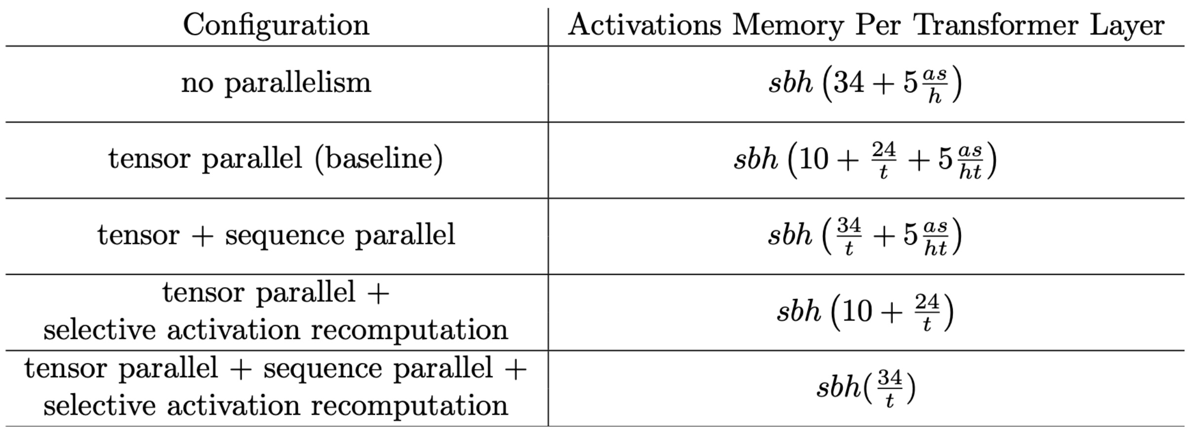
The minimum memory usage you can easily achieve is \(sbh \\cdot \\frac{34}{t}\), which is often used in transformer arithmetic formulas when calculating activation memory requirements. You’ll frequently see expressions like \(sbh \\cdot 34\), and with \(t\) tensor parallelism, you divide by \(t\) because this represents the easy minimum you can achieve for that kind of memory usage. For more complicated computation graphs beyond a single linear chain, tensor parallelism operates purely layer-wise and doesn’t really care about dependencies. Pipeline parallelism might offer opportunities for increased parallelization if there are multiple branches, but the analysis applies to each layer individually. This comprehensive approach to memory optimization through various parallelization strategies gives us the tools needed to train truly massive models efficiently.
10. 3D Parallelism and Scaling Strategies
Comprehensive Parallelism Overview
Now that we’ve covered the fundamental parallelism strategies, let’s explore some advanced parallelism approaches that extend beyond the basic techniques. The first one I want to talk about is context parallel or ring attention. You may have heard the term ring attention before – this is a way of essentially splitting up both the computation and the activation cost of computing really large attention. Where essentially, you’re just going to pass keys and values around different machines. So each machine is responsible for a different query, and the keys and values are going to travel from machine to machine in a ring-like fashion in order to compute your \(KQV\) inner products. The cool thing here is you already know how to do this because you’ve done the tiling for flash attention. So you know that attention can be computed in this kind of online tile-by-tile way, and that’s kind of what’s happening in ring attention.
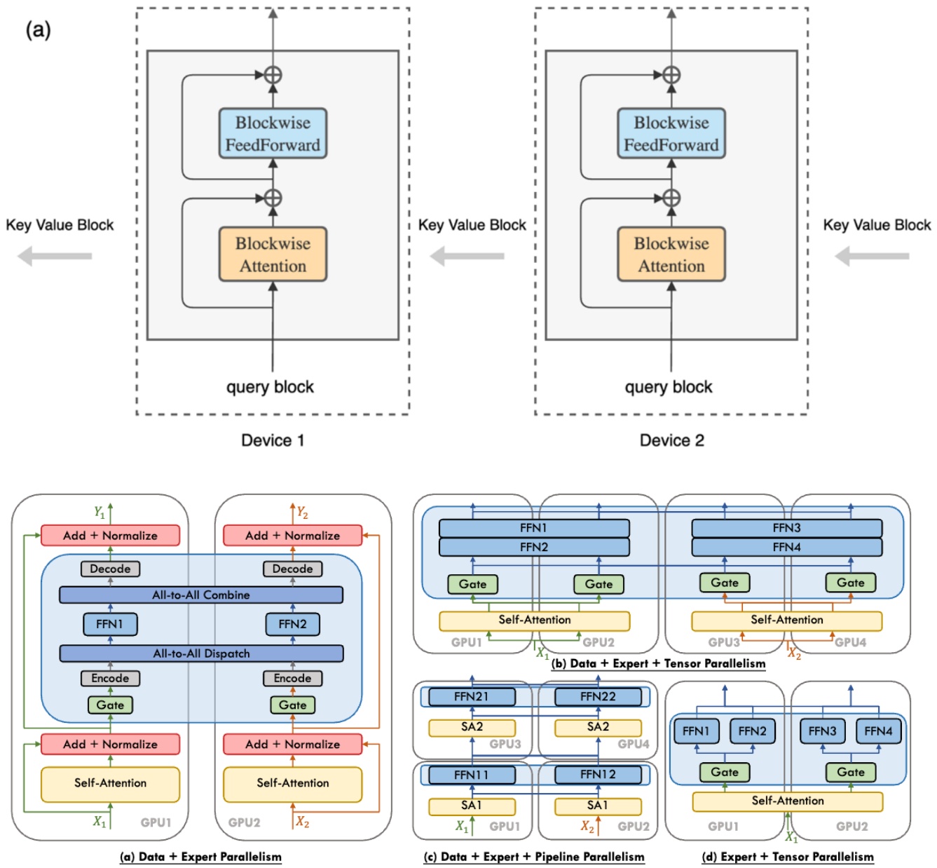
The other strategy, which now that you know tensor parallel is pretty straightforward, is expert parallelism. Expert parallelism, you can kind of think of as almost like tensor parallel in the sense that you’re splitting up one big MLP into smaller expert MLPs, let’s say, and then scattering them across different machines. The key difference with expert parallelism is that the experts are sparsely activated, and so you have to think a little bit about routing. The routing is not going to be sort of as predictable as the all-to-all communication that we had before in tensor parallel, because now maybe one expert is overloaded. Your networking is going to be a little bit more complicated, but otherwise conceptually, you’re living in kind of the same world as tensor parallel for expert parallels.
💡 Parallelism Strategy Comparison
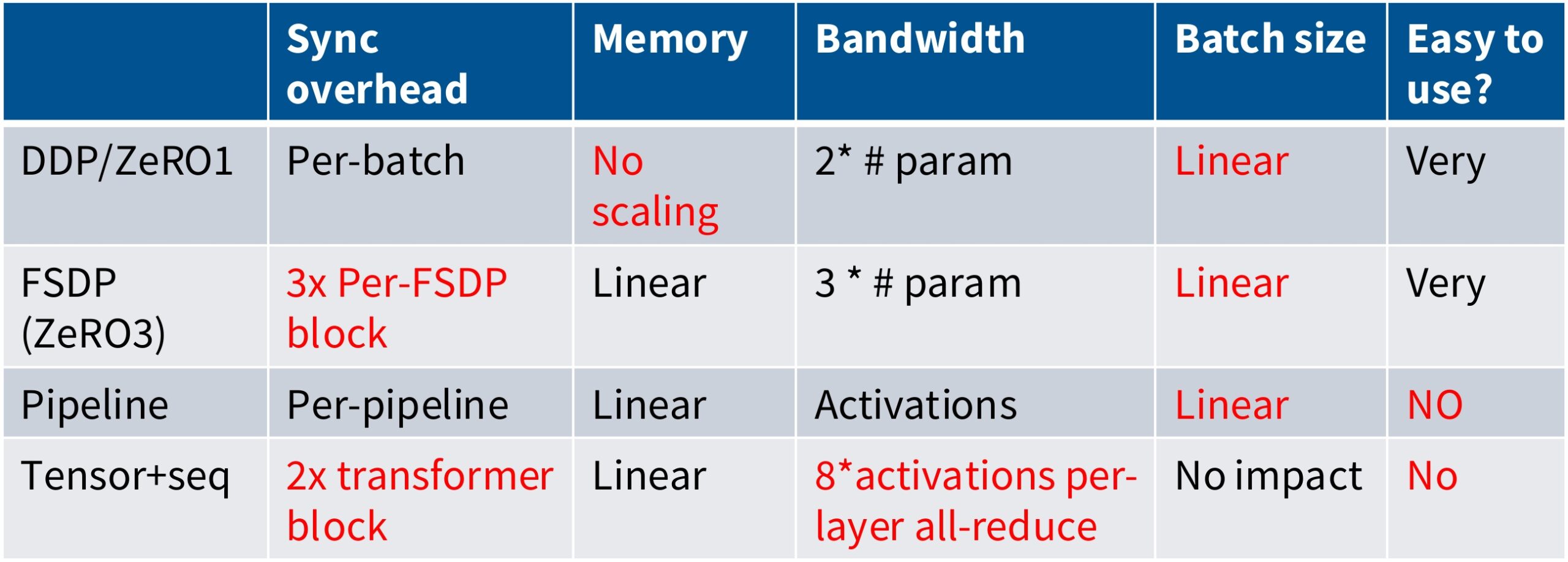
So just to recap all the things we talked about, I’ve made a little small table of the different kinds of strategies that we have. We have DDP and ZeRO-1, which is kind of the naive data parallelism thing that you do – here, you have some overhead per batch, you have no memory scaling, reasonable bandwidth properties, but you consume batch size in order to be able to do this. You need big batch sizes to have big data parallelism. You have FSDP, which is kind of like a nicer version of ZeRO-1 in the sense that you can get memory scaling, but you’re going to pay overhead across sort of different layers. And so now you’ve got higher communication cost and you’ve got potentially synchronization barriers that lead to poor utilization. Pipeline parallel is nice in that we no longer have this dependence on this per batch aspects, but we can get linear memory scaling. But we have sort of another issue, which is this also consumes batch size and it’s horrendous to sort of set up and use. And so a lot of people like to avoid pipeline parallelism if it’s possible. And finally, tensor parallelism is very high cost in terms of bandwidth and the amount of synchronization you need to do, but this has this really nice property that has no impact on batch sizes. So it’s like kind of the one parallelism strategy you can use that has no cost in terms of your global batch size, which is nice.
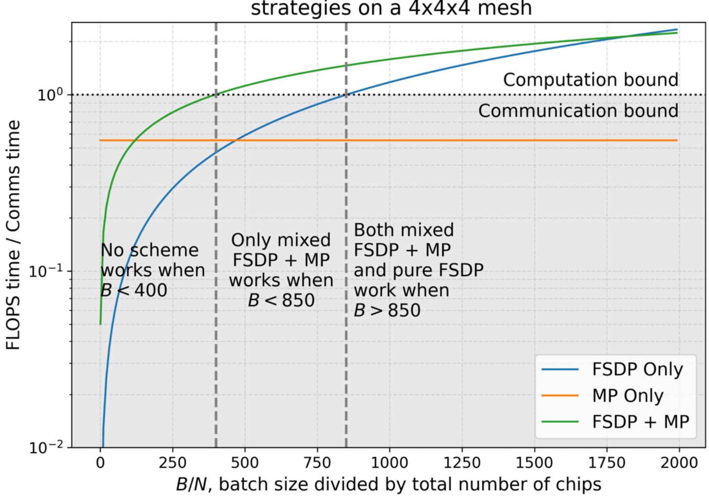
We have to balance a number of limited resources. We have memory, which is one resource. We have bandwidth and compute, which is another resource. And then we have batch size, which is kind of an unconventional resource, but one that you should really think of as a limited thing that you can spend on different aspects of these to improve your efficiency. The key quantity as I was saying before is the batch size. And depending on the ratio of batch size to the number of GPUs you have, different kinds of parallelism become optimal. You can kind of see if your batch size is too small, you have lots of GPUs and really tiny batch sizes, then there is no way for you to be efficient. You’re always communication bound. As you sort of get more and more batch size, eventually you can get to a point where if you mix both FSDP, so ZeRO stage 3 and MP, which in this case is tensor parallel, you can actually get basically to a place where you’re compute bound. So now you’re not spending sort of wasting your flops waiting for communication. And then finally, if you get to a point where your batch sizes are big, then you can just get away with pure data parallel. Pure FSDP is going to get you into a regime where the time you spend doing computation is higher than the time you spend in communication. This understanding of resource trade-offs leads us naturally to how we can combine these strategies effectively.
3D Parallelism Integration
Building on our understanding of individual parallelism strategies and their trade-offs, let’s see how to combine them systematically. When you put these all together, you end up with what people call 3D or 4D parallelism – I think I’ve heard the term 5D parallelism recently. But now you can put it all together, the different dimensions of parallelism. And this is a really simple rule of thumb. The first thing you have to do is you have to fit your model and your activations in memory. If you don’t do that, you just cannot train. So until your model fits in memory, we have to split up our model. We’re going to do tensor parallelism, and we know that up to the number of GPUs per machine, that’s very efficient, that’s very fast. So we’re going to do tensor parallel up to that point.
If your model still doesn’t fit after tensor parallel 8, you’ll need to apply pipeline parallel. Pipeline parallel is sort of slow, but it gets you additional memory savings. After you’ve done tensor parallel and potentially pipeline parallel to fit your model in memory, you should use data parallel to consume the remaining batch size that you have left. This is the canonical ordering of parallelization strategies that people use in practice – tensor parallel first within nodes, pipeline parallel across nodes if needed, and data parallel to utilize remaining resources and batch size.
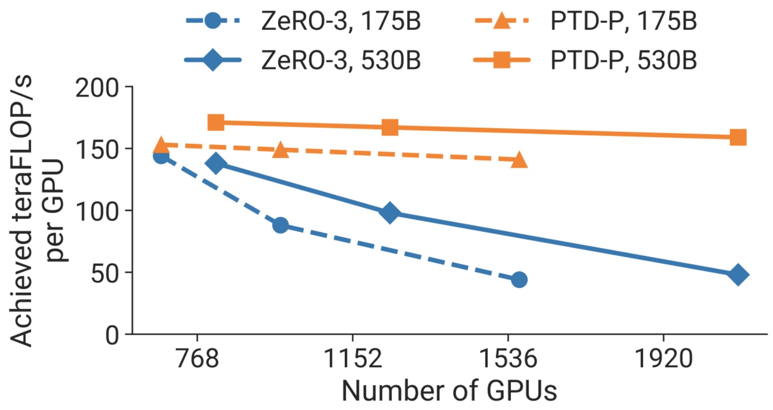
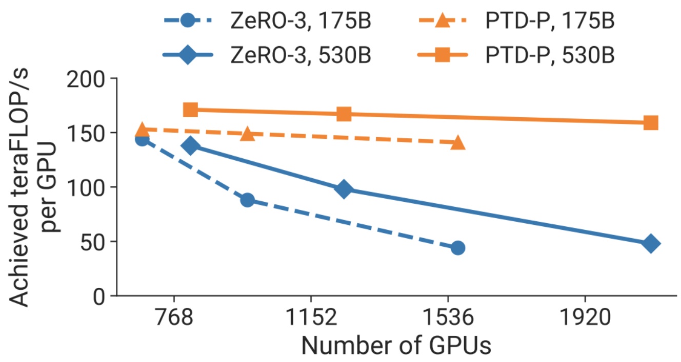
The results from real-world implementations validate this approach. Looking at actual scaling numbers from research, you can see the progression across model sizes. At 1.7B parameters, they use minimal parallelization. At 8.3B parameters, they introduce tensor parallel of 4. By 39B parameters, they’re using tensor parallel of 8 and pipeline parallel of 4. The largest model at 1008B parameters uses tensor parallel of 8 and pipeline parallel of 32. These numbers demonstrate how the parallelization strategy adapts systematically as model size increases.
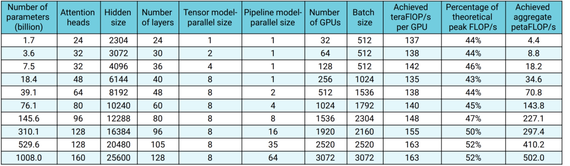
Optimal Scaling Configuration
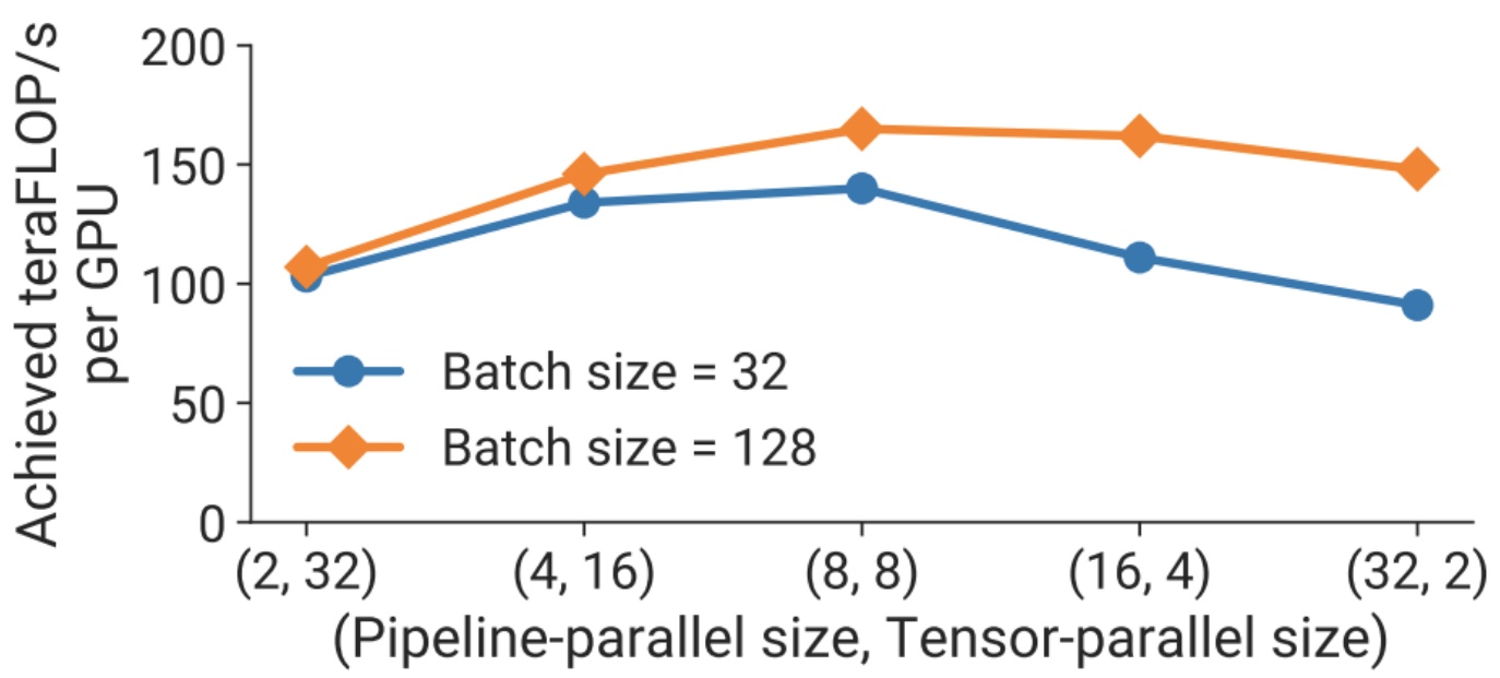
The results from these systematic 3D parallelism approaches reveal some clear patterns about what configurations work best. When implementing careful 3D parallelism, you’ll observe remarkably flat overall achieved FLOPS per GPU, which delivers linear scaling in total aggregate throughput as you add more GPUs – and that’s exactly what we want to see. The data consistently shows that tensor parallel size of 8 is often optimal across different configurations.
Looking at the relationship between pipeline parallel size and tensor parallel size, you’ll notice that going to an \(8 \\times 8\) configuration with batch sizes of 32 or 128 proves optimal. Even when you’re working with smaller batch sizes, that tensor parallel size of 8 remains the sweet spot. When parallelizing across 64 machines, this \(8 \\times 8\) configuration consistently delivers the best results.
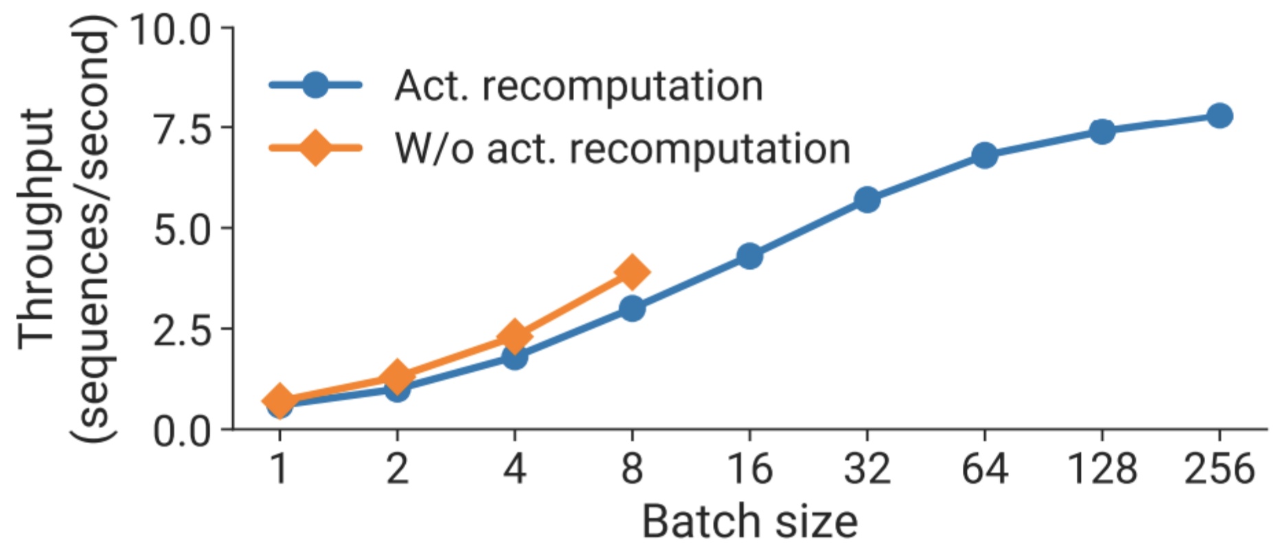
Here’s where activation recomputation becomes particularly interesting – it enables larger batch sizes, and remember that larger batches can help you mask overhead for pipeline parallelism. So even though activation recomputation requires more FLOPS, it can actually pay for itself through improved throughput. This is similar to the story we’ve already seen play out with flash attention, where the computational trade-off ultimately delivers better performance. With configurations like \(t=8\) and \(p=16\), activation recomputation enables larger batches that significantly improve overall throughput.
11. Production Model Implementations
Recent Large Model Strategies
Now let’s examine how these parallelization concepts translate into real production systems. I’ve gone through several recent papers to look at examples of what people’s parallelization strategies are, and let me walk you through some concrete implementations. The Olmo and Dolma papers provide excellent case studies – they use FSDP (Fully Sharded Data Parallel) for their 7 billion parameter model, which gives us insight into how modern large-scale training actually works in practice.
Their approach centers on the ZeRO optimizer strategy via PyTorch’s FSDP framework, which is really clever because it reduces memory consumption by sharding the model weights and their corresponding optimizer state across GPUs. At the 7B scale, this enables training with a micro-batch size of 4096 tokens per GPU on their hardware setup. What’s interesting is how they handle batch sizing across different model scales – for OLMo-1B and -7B models, they use a constant global batch size of approximately 4M tokens, which translates to 2048 instances each with a sequence length of 2048 tokens. For their larger OLMo-65B model, they implement a more sophisticated batch size warmup strategy that starts at approximately 2M tokens and doubles every 100B tokens until reaching approximately 16M tokens.
To improve throughput, they employ mixed-precision training through FSDP’s built-in settings and PyTorch’s amp module. This is where the implementation gets really nuanced – the amp module ensures that certain operations like the softmax always run in full precision to improve stability, while all other operations run in half-precision with the bfloat16 format. Under their specific settings, the shared model weights and optimizer state local to each GPU are kept in full precision, but the weights within each transformer block are only cast to bfloat16 when the full-sized parameters are materialized on each GPU during the forward and backward passes. Importantly, gradients are reduced across GPUs in full precision, which maintains training stability while still getting the memory and speed benefits of mixed precision. This foundational approach sets the stage for even more sophisticated strategies we see in other recent models.
DeepSeek and Yi Model Approaches
Building on these foundational techniques, when we examine the parallelization strategies employed by leading Chinese language models, we see some fascinating variations in approach. DeepSeek’s initial paper implemented ZeRO stage 1 with tensor, sequence, and pipeline parallelism – a fairly standard but effective combination. However, DeepSeek V3 takes a notably different path, utilizing 16-way pipeline parallelism combined with 64-way expert parallelism (which functions similarly to tensor parallelism) and ZeRO stage 1 for their data parallelism strategy. This shift toward expert parallelism reflects the growing adoption of mixture-of-experts architectures in large-scale model training.
The Yi model family demonstrates similar strategic thinking in their parallelization choices. The base Yi model employs ZeRO stage 1 combined with tensor and pipeline parallelism, following established best practices. However, Yi-Lightning (2025) makes a crucial architectural decision by replacing tensor parallelism with expert parallelism, specifically because they’re implementing a mixture-of-experts (MOE) approach. This substitution makes perfect sense – when you have expert layers, expert parallelism becomes the natural choice for distributing computation efficiently across available hardware.
The technical implementation details reveal sophisticated optimization strategies. Both model families leverage the HAI-LLM training framework, which integrates data parallelism, tensor parallelism, sequence parallelism, and 1F1B pipeline parallelism as implemented in Megatron. They employ flash attention techniques to improve hardware utilization and use ZeRO-1 to partition optimizer states across data parallel ranks. Memory and communication restrictions represent the two major technical challenges in large-scale model training, requiring integrated solutions that go beyond simply adding more GPUs.
To address these challenges, the teams implement several key optimizations: ZeRO-1 removes memory consumption by partitioning optimizer states across data-parallel processes, while tensor parallel combined with pipeline parallel within each compute node avoids inter-node communication bottlenecks. The 3D parallel strategy is carefully designed to avoid activation checkpointing and minimize pipeline bubbles. Additional techniques include kernel fusion methods like flash attention and JIT kernels to reduce redundant global memory access, topology-aware resource allocation to minimize communication across different switch layers, and training in bf16 precision while accumulating gradients in fp32 precision for improved stability. These strategies become even more critical when we look at truly massive scale implementations.
Llama3 405B Training Infrastructure
Speaking of massive scale, if you’re interested in state-of-the-art distributed training with lots of practical details, Llama 3’s report is actually really fascinating to read. They provide extensive detail about their networking approach and implementation strategies. What you’ll see is exactly the kind of parallelism hierarchy I mentioned before – they use tensor parallel (\(TP\)) of eight, context parallel (\(CP\)), pipeline parallel (\(PP\)), and data parallel (\(DP\)) happening in these first two phases. You can even ignore the first stage here because that’s the small batch size training they did for stability purposes.
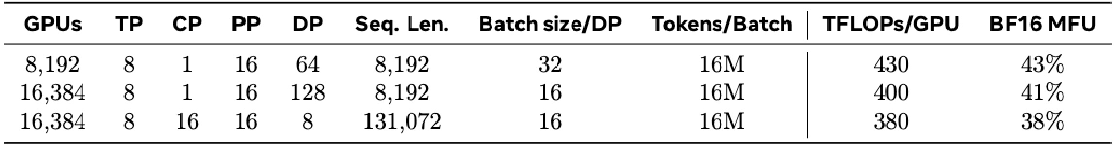
Network-aware parallelism configuration. The order of parallelism dimensions, \([TP, CP, PP, DP]\), is optimized for network communication. The innermost parallelism requires the highest network bandwidth and lowest latency, and hence is usually constrained to within the same server. The outermost parallelism may spread across a multi-hop network and should tolerate higher network latency. Therefore, based on the requirements for network bandwidth and latency, we place parallelism dimensions in the order of \([TP, CP, PP, DP]\). \(DP\) (i.e., FSDP) is the outermost parallelism because it can tolerate longer network latency by asynchronously prefetching sharded model weights and reducing gradients. Identifying the optimal parallelism configuration with minimal communication overhead while avoiding GPU memory overflow is challenging. We develop a memory consumption estimator and a performance-projection tool which helped us explore various parallelism configurations and project overall training performance and identify memory gaps effectively.
Looking at their rationale for the parallelism strategy, you see exactly what I had explained before – you want to implement \(TP\), \(CP\), pipeline parallel, and \(DP\) in that specific order based on the amount of bandwidth required. Data parallel can tolerate those long network latencies because you can do asynchronous fetching of sharded model weights. So they’re using precisely the strategy I described to train some of the biggest models in existence.
🔴 Hardware Reliability at Scale
Critical reality: Here’s a funny but important side note about Llama 3 that you may have heard in casual conversations – there are lots of GPU failures when you train models at this massive scale. They experienced 148 interruptions from faulty GPUs alone, totaling about 30% of all their training interruptions. They also dealt with unplanned maintenance issues across 32 different instances. When you’re training a model this enormous, you need not just the algorithms I’ve discussed, but also fault-tolerant architectures to handle these inevitable hardware issues.
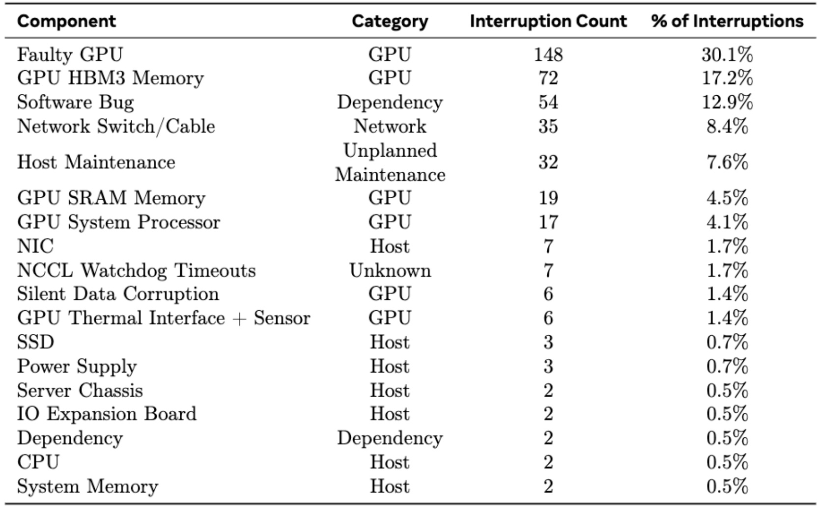
What’s even scarier than explicit hardware failures, according to various stories I’ve heard from practitioners, is the silent threat of data corruption. About 78% of unexpected interruptions during their 54-day training period were attributed to confirmed or suspected hardware issues. This reality check shows that when you’re operating at this scale, robust infrastructure and monitoring systems become just as critical as the mathematical foundations of your training algorithms. This brings us to an interesting alternative approach that addresses some of these reliability concerns.
Gemma 2 TPU Training Implementation
Let me wrap up with a compelling example from Gemma 2, which showcases TPU training implementation at scale and offers a different perspective on hardware reliability. Unlike GPUs that can silently fail and corrupt your entire training run with garbage data, TPUs offer more reliable scaling capabilities. The Gemma 2 team leverages ZeRO-3 optimization (roughly equivalent to Fully Sharded Training Protocol), combined with both model parallelism and data parallelism. This hybrid approach allows TPUs to stretch model parallelism capabilities much further than traditional GPU setups, making it an ideal choice for large-scale language model training.
The specific training configurations for Gemma 2 demonstrate the power of this approach across different model sizes. For the 2B model, they use a \(2 \\times 16 \\times 16\) configuration of TPUv5e chips, totaling 512 chips with 512-way data replication and 1-way model sharding. The 9B model scales up to an \(8 \\times 16 \\times 32\) configuration of TPUv4 chips (4096 total) with 1024-way data replication and 4-way model sharding. The largest 27B model requires an \(8 \\times 24 \\times 32\) configuration of TPUv5p chips, totaling 6144 chips with 768-way data replication and 8-way model sharding.
The technical infrastructure behind this scaling is quite sophisticated. The optimizer state gets further sharded using ZeRO-3 techniques, and for scales beyond a single pod, they perform data-replica reduction over the data center network using the Pathways approach. They also leverage the ‘single controller’ programming paradigm from JAX and Pathways, along with the GSPMD partitioner for training step computation and the MegaScale XLA compiler for optimization.
The key takeaway here is that scaling beyond a certain point absolutely requires multi-GPU, multi-node parallelism – there’s simply no single solution that works for everything. You want to combine all three approaches (tensor parallelism, pipeline parallelism, and data parallelism) to leverage their respective strengths. Fortunately, there are simple and interpretable rules of thumb for how you might execute this parallelism in practice, and the examples we’ve covered provide concrete roadmaps for implementing these strategies at scale.
These lecture notes are based on the Stanford Course: LLMs from Scratch, 2025. Lecture 7, Youtube.
Key Takeaways
- Hardware Architecture Matters: Understanding GPU networking hierarchies and communication primitives (all-reduce, reduce-scatter, all-gather) is fundamental to choosing effective parallelization strategies.
- Three Core Parallelization Dimensions: Data parallelism (ZeRO stages 1-3), model parallelism (tensor and pipeline), and activation parallelism (sequence parallel) each address different bottlenecks in memory and computation.
- ZeRO Optimization: Progressive sharding of optimizer states, gradients, and parameters can reduce memory consumption from 120GB to under 2GB per GPU while maintaining similar communication costs.
- Tensor Parallelism Sweet Spot: Use tensor parallelism up to 8 GPUs within a single node where high-speed interconnects make communication efficient; beyond 8 devices, performance degradation becomes severe.
- Pipeline Parallelism Trade-offs: While conceptually intuitive, pipeline parallelism is complex to implement and consumes batch size, but necessary when models won’t fit in memory even with tensor parallelism.
- 3D Parallelism Integration: Combine strategies systematically: tensor parallel first (within nodes), pipeline parallel if needed (across nodes), then data parallel (to utilize remaining batch size).
- Production Reality: Real-world implementations like Llama 3, DeepSeek, and Gemma 2 use sophisticated combinations of all techniques, with careful attention to hardware topology, fault tolerance, and memory-compute-batch size trade-offs.