LLM_log #031: Long Context in Practice — Training Recipes (RoPE, YaRN, NoPE), KV and Prompt Caching, and Context Compaction
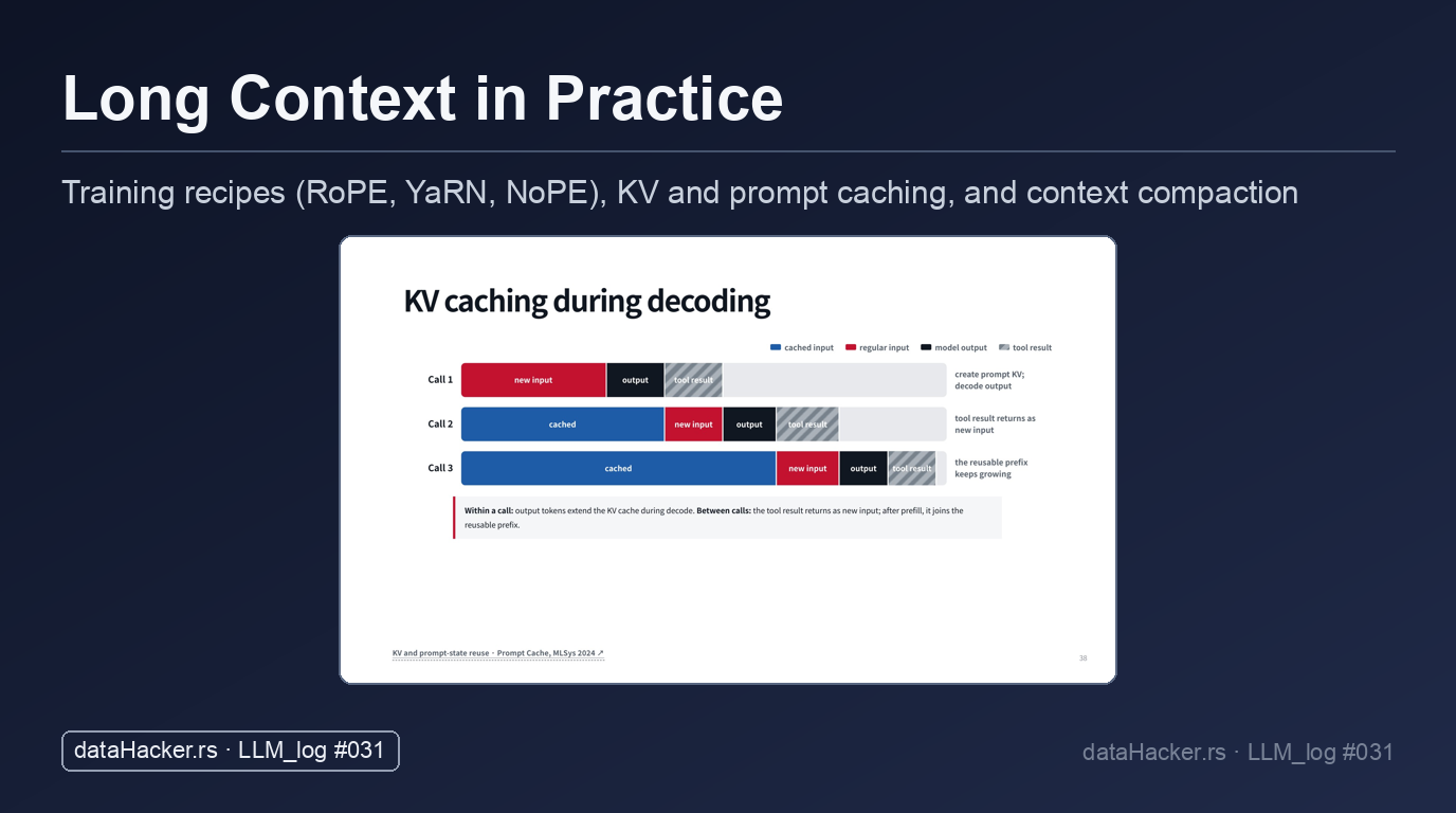
Long Context in Practice — Training Recipes (RoPE, YaRN, NoPE), KV and Prompt Caching, and Context Compaction
Highlights: In this second part of the long-context lecture from CMU’s 11-768 AI Agents course (Fall 2026, Graham Neubig), the focus shifts from model architecture to everything that surrounds it: how long-context models are trained, served, and kept affordable. We walk through staged short-to-long training pipelines, positional encoding choices from RoPE interpolation to NoPE, the serving stack built around KV caching, and context compaction framed as state estimation over agent history.
- Staged adaptation: Coherent 128K-token documents are scarce, so models are trained in stages — short pretraining at 4K–8K, continued training at 32K–128K, then long adaptation out to 1M tokens with synthetic curricula.
- NoPE and RoPE extension: Causal masking already distinguishes repeated tokens by position, which is why several models drop positional encodings entirely, while others stretch RoPE through uniform position interpolation or YaRN’s frequency-selective scaling with attention temperature correction.
- Context parallelism: Past roughly 32K tokens of context, splitting the sequence dimension across devices (Ring Attention, Megatron context parallelism) becomes important — and the kernel often does not exist yet for newer recurrent layers.
- KV caching internals: PagedAttention borrows virtual memory paging to eliminate GPU fragmentation, RadixAttention stores prefixes in a radix tree for reuse, and cache-aware routing scores workers by reusable prefix minus queue penalty.
- Cache economics: Cached tokens typically cost one tenth of uncached ones and output tokens five times more, giving roughly a 50× spread — so mutating system prompts, appending timestamps, or switching models mid-run is expensive.
- Compaction as state estimation: A compactor maps history into a bounded working state that must preserve future action distributions, with anchors, checkpoints and a raw recent tail — and the OpenHands SWE-bench case shows why offline benchmarks miss repeated compaction drift.
Tutorial Overview:
- Staged Adaptation Pipelines for Extended Contexts
- Long-Context Data Sources and Pretraining Mixtures
- Positional Encodings and the Case for NoPE
- RoPE Context Extension via Position Interpolation
- Frequency-Selective YaRN and Model Extension Paths
- Context Parallelism and Distributed Training
- KV Caching Mechanics and Prefix Reuse
- Paged Memory Allocation and Prefix Trees
- Cache-Aware Routing and Serving Infrastructure Metrics
- Prefix Caching Economics and API Pricing Models
- Prompt Engineering for Prefix Cache Preservation
- Context Compaction as Agent State Estimation
- Context Compaction Policies, Anchors, and Repeated Compaction Drift
- The Long-Context System Stack Across Agent Architectures
- Summary
1. Staged Adaptation Pipelines for Extended Contexts
1.1 Short-to-Long Progressive Training
With efficiency techniques in place, models can scale to as many as one million tokens. The harder problem is training a long-context model in the first place, and the obstacle is data. If we want a model that handles 128K tokens or more, there simply is not much text on the internet that exists as 128K coherent tokens.
That is an enormous amount of text, far longer than the vast majority of Wikipedia articles. At that scale we are talking about the length of an entire book, and there are not many full books readily available online.
Because coherent long data is scarce and expensive to train on from scratch, practitioners follow a staged curriculum. We begin with short pre-training at standard lengths of 4K to 8K tokens, where data is abundant and compute is cheap. Next comes continued training at 32K to 128K on long documents and packed sequences. Finally, long adaptation pushes to 128K+ tokens using task traces and synthetic curricula.
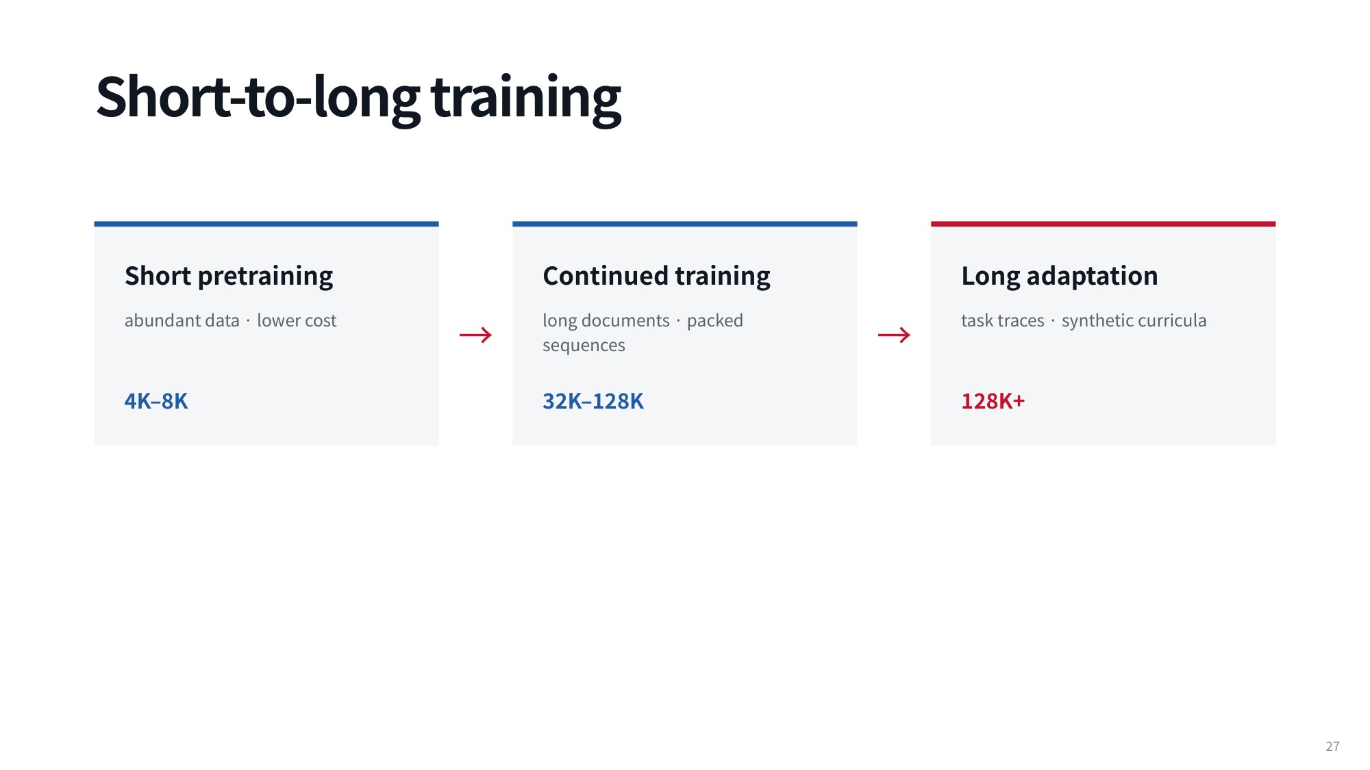
Fig 1. Short-to-long training
One nuance about data preparation deserves attention. Packed sequences appear in the pipeline because they are useful for hardware and throughput efficiency, but as Graham Neubig points out in the CMU lecture, they do little for learning long-context behavior. Concatenate ten unrelated documents into one sequence and the model never learns to attend across them — and arguably it should not.
Genuinely coherent, extended data is what adapts a model to very long contexts. That means carefully structured adaptation schedules working alongside the architectural recipes that keep standard attention out of its quadratic bottleneck.
2. Long-Context Data Sources and Pretraining Mixtures
2.1 Natural Long Documents and Agent Trajectories
Where does long-context training data actually come from? Mostly from documents that are already long. Across models such as Kimi K3, GLM-5, Nemotron 3 Ultra, and DeepSeek V4, the pretraining mixtures draw on cleaned-up sample documents, full repository files, pull request issues, and video documents.
These formats matter because they expose the model to realistic long-horizon documents and structured agent trajectories from the very beginning of training.
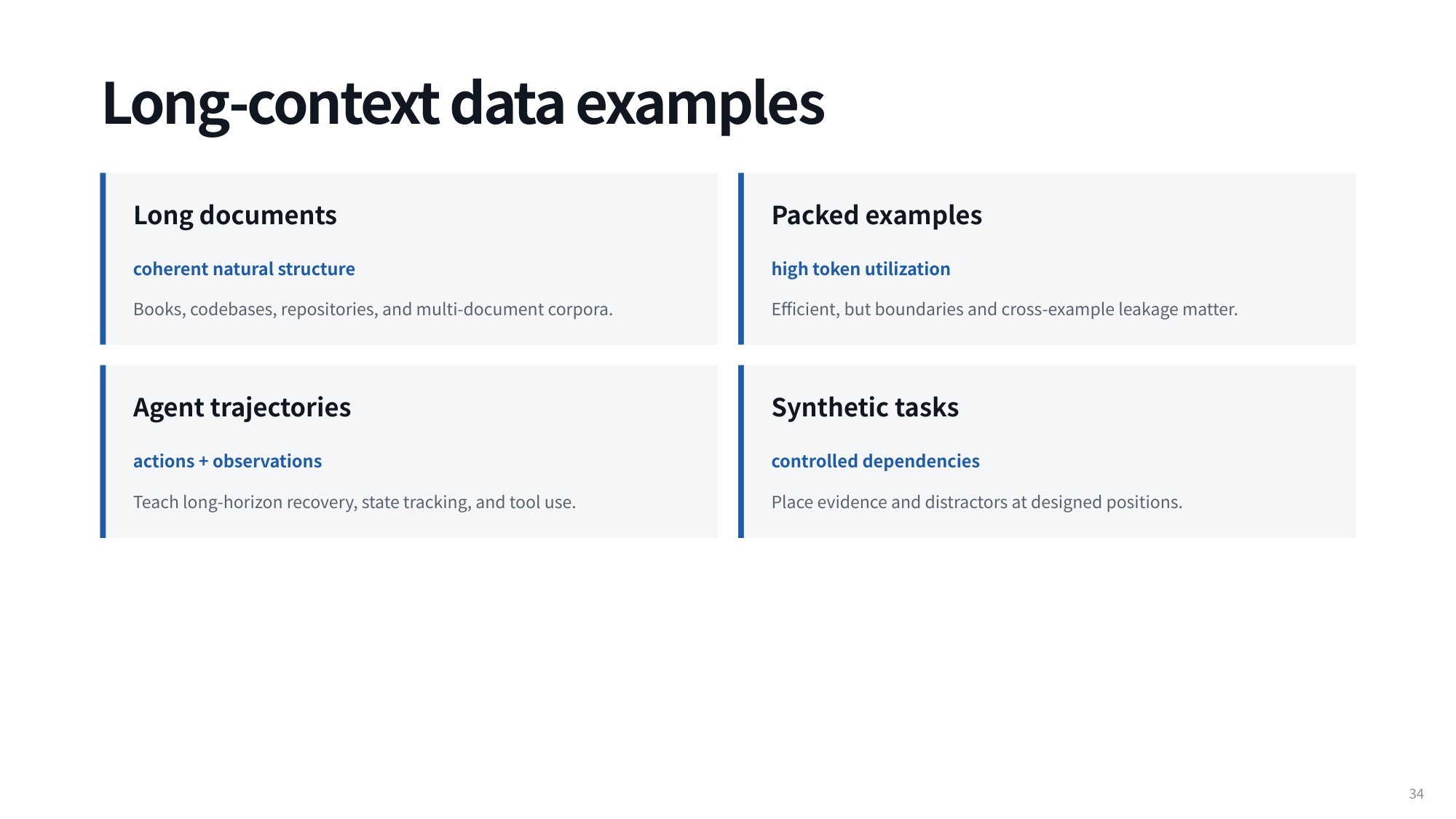
Fig 2. Long-context data examples
2.2 Document and Trajectory Characteristics
Beyond raw trajectories and repository files, the mixtures lean on specific document types: scientific papers, technical reports, and long-document question answering benchmarks.
Natural data is not the whole story. Teams also generate a wide variety of synthetic tasks built specifically to reinforce reasoning over extended inputs.
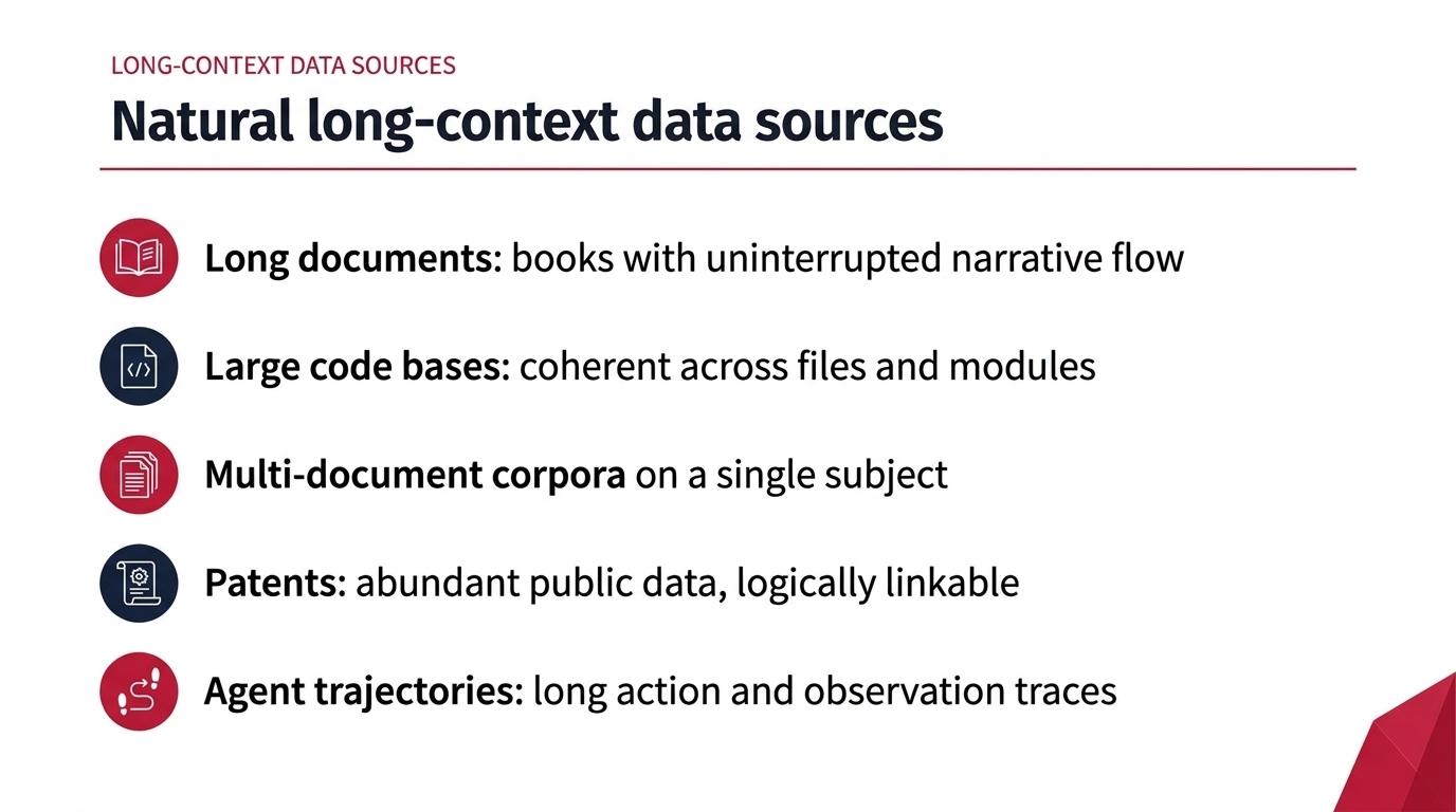
Fig 3. Natural long-context data sources
2.3 Mixtures for Progressive Scaling and Staged Adaptation
Open model companies sit in an interesting position. They are practically obligated to publish their architectural details, because you cannot run a model without them. What stays behind closed doors is the data mix and the training strategy.
That is why granular information is scarce here. Still, every model discussed above discloses at least a high-level view of the mixture behind its long-context capability.
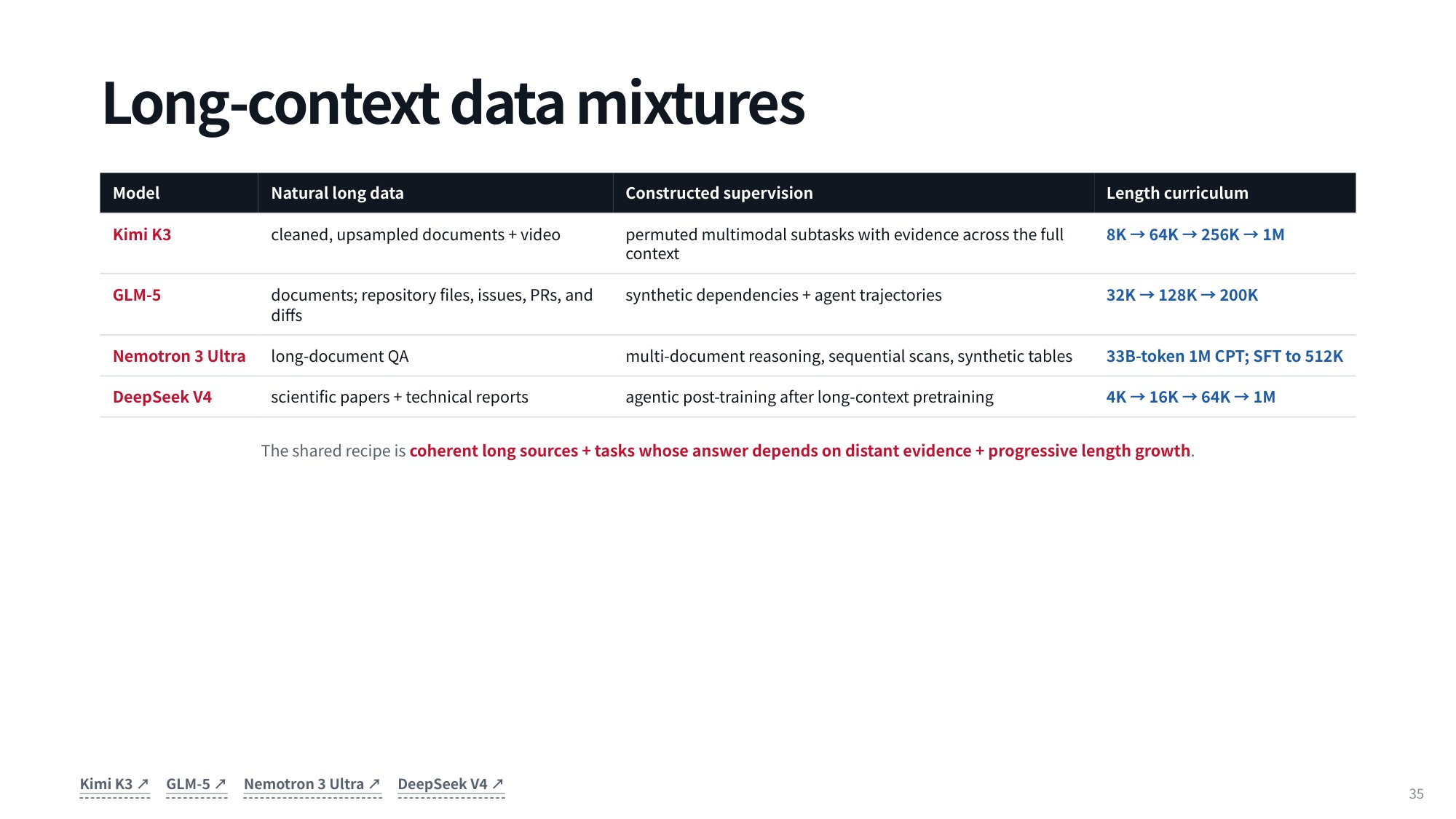
Fig 4. Long-context data mixtures
The common ingredients are consistent: cleaned-up sample documents, video documents, repository files, pull request issues, long-document question answering datasets, scientific papers, technical reports, and synthetic tasks for long-context reasoning. On top of that, teams typically use a staged adaptation curriculum that scales context length across training stages, moving through 8K → 64K → 256K and up to 1M tokens.
3. Positional Encodings and the Case for NoPE
How should a model know where a token sits in a sequence? The classical answer is absolute positional encodings. For every token ID (x_t), the model looks up an embedding vector (E[x_t]) in the embedding table, then adds a dedicated position vector (p_t) to it.
That position vector comes from a deterministic function built on sines and cosines. With (\ell) indexing the sinusoid pairs across the embedding dimension (d), varying geometric frequencies (\omega_\ell) give every time step (t) its own distinct coordinate pattern.
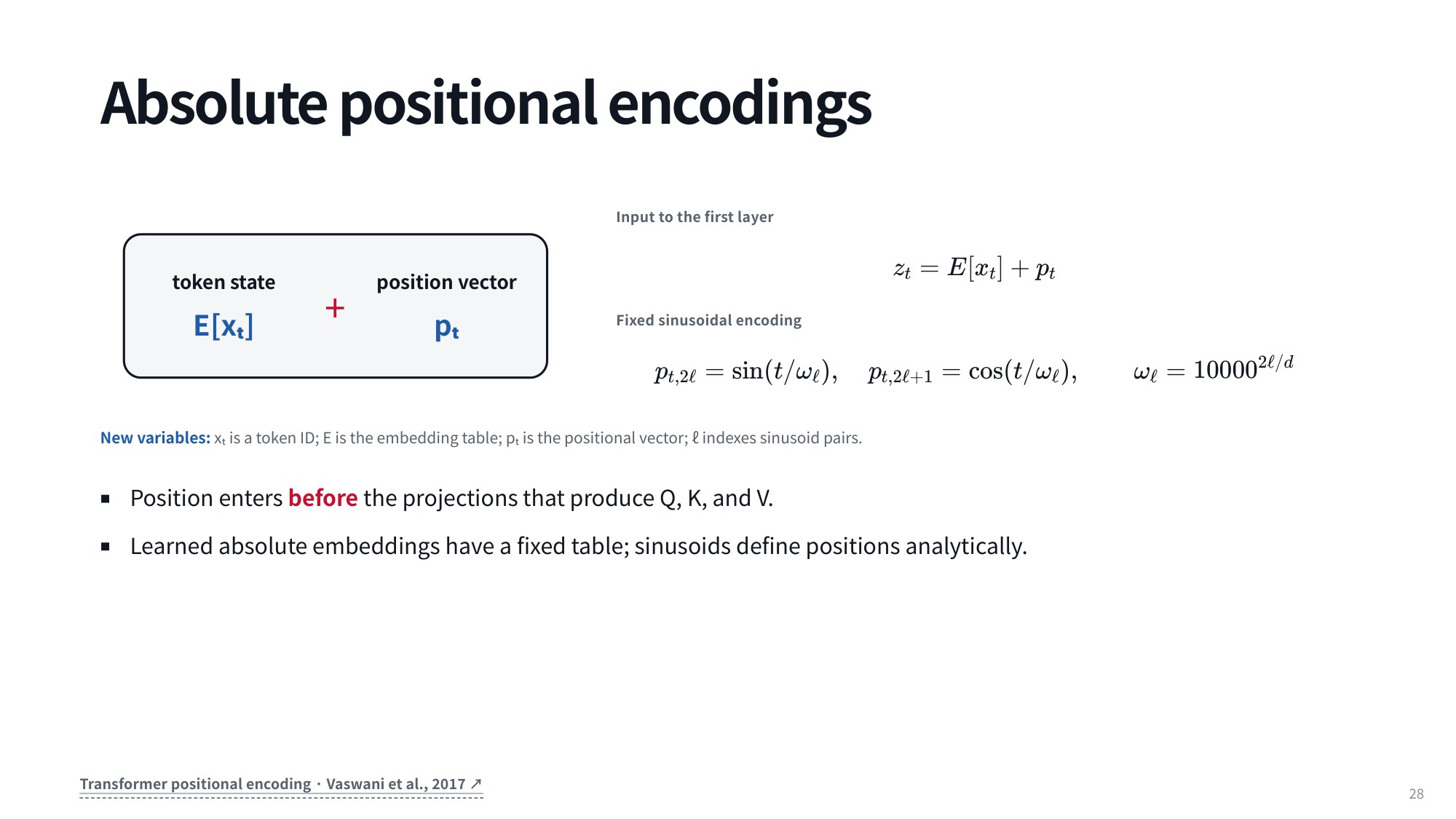
Fig 5. Absolute positional encodings
[z_t = E[x_t] + p_t]
[p_{t,2\ell} = \sin(t/\omega_\ell), \quad p_{t,2\ell+1} = \cos(t/\omega_\ell), \quad \omega_\ell = 10000^{2\ell/d}]
3.1 From RoPE to NoPE
If you work with modern architectures, you have almost certainly met RoPE (Rotary Position Embedding).
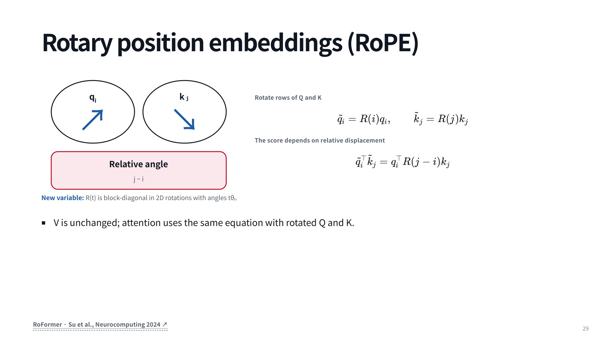
Fig 6. Rotary position embeddings (RoPE)
RoPE is mathematically elegant. Its designers wanted an encoding determined entirely by the relative distance between two tokens: where a token happens to sit in a document should not decide whether two tokens attend to each other, only their offset should.
The formulation works well, and a large share of today’s foundation models depend on it. We will skip the full derivation here, but the trick rests on 2D rotations and complex numbers.
There is a compelling alternative: NoPE, meaning no positional encodings at all. Introductory transformer courses usually warn that positional encodings are mandatory, because otherwise a token at position one and an identical token at position five would share the same internal representation. On that assumption, a sentence like “this is a cat, but this is not a cat” would make the model attend to both occurrences of “cat” by exactly the same amount. That concern was valid for the original transformer, but it no longer holds.
Why not? Early transformers were mostly encoder-decoder models, where bidirectional encoders processed all input tokens at once and the decoder produced the output. Modern autoregressive models use strict causal masking instead.
Look at what causal masking does to the query-key dot products. “cat” at position two can only attend to the single preceding token, while “cat” at position five attends across all four preceding tokens. The two instances acquire completely distinct contextual representations from the very first layer.
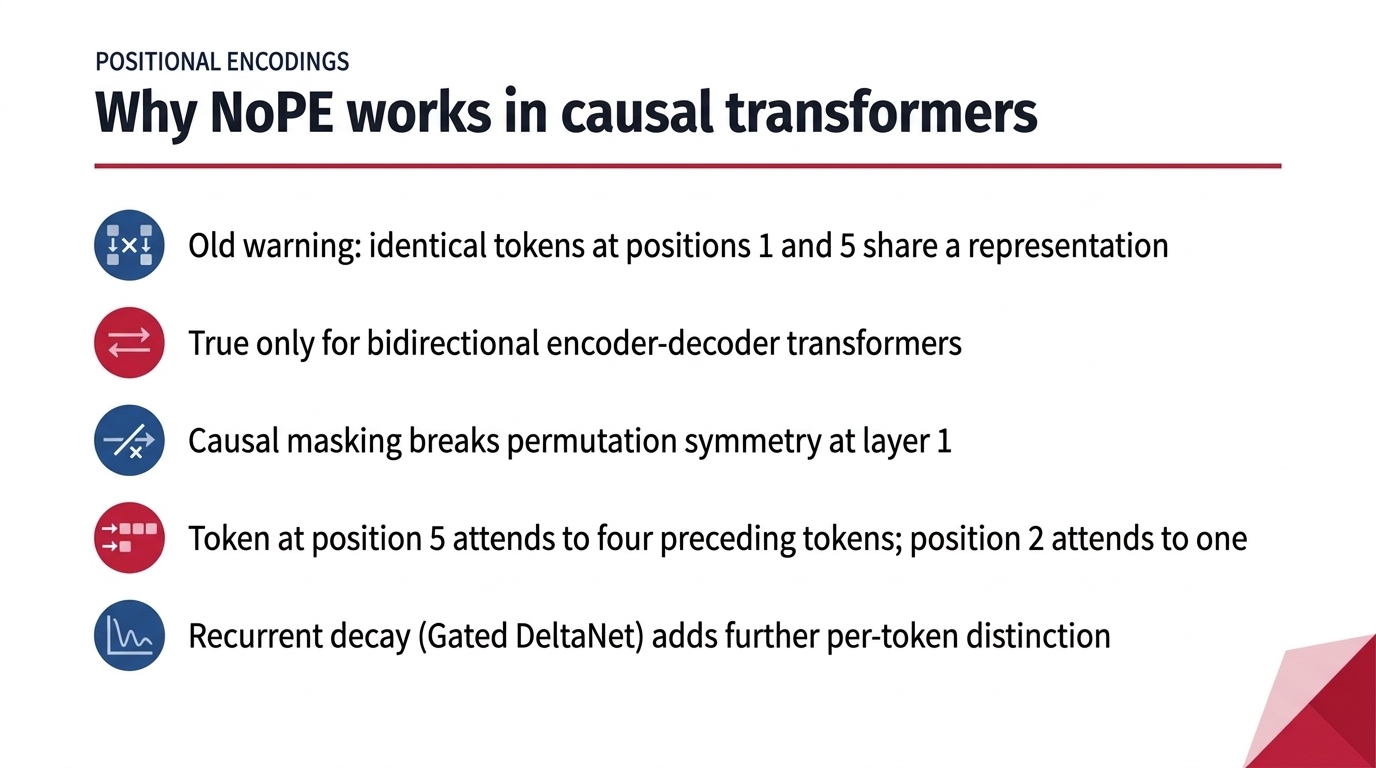
Fig 7. Why NoPE works in causal transformers
3.2 NoPE in Autoregressive Models
In autoregressive transformers, sequence order falls out of the causal computation or recurrent dynamics rather than from an explicit position vector (p_t) or a rotary transformation (R(t)). The representation is just the embedding lookup for the incoming token (x_t):
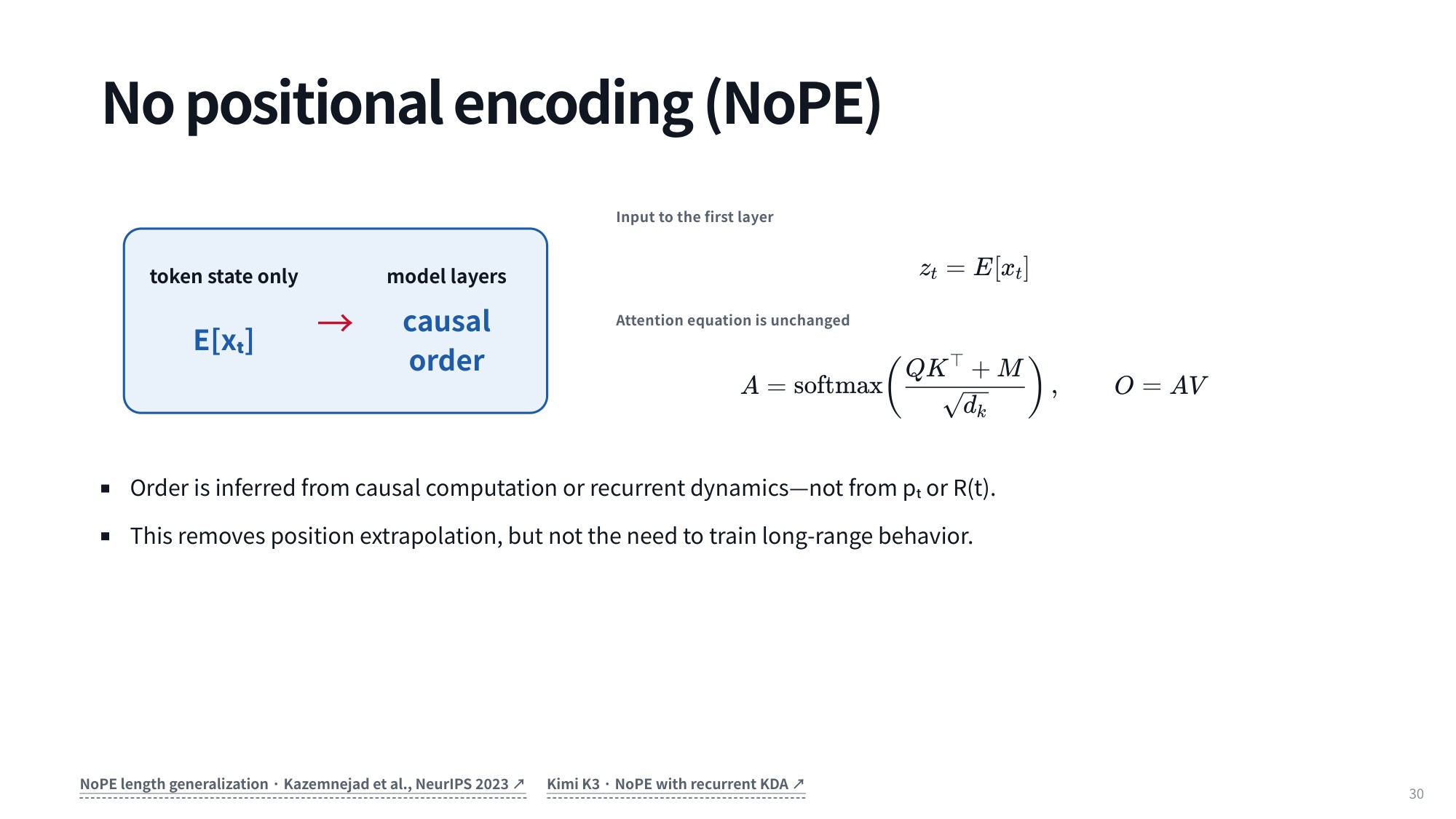
Fig 8. No positional encoding (NoPE)
[z_t = E[x_t]]
The autoregressive mask (M) restricts each token to earlier positions, which distinguishes identical words purely by the tokens that preceded them:
[A = \mathrm{softmax}\left(\frac{QK^{\top}}{\sqrt{d_k}} + M\right), \quad O = AV]
Non-autoregressive transformers are a different story. When every token attends bidirectionally to every other token, the operation is permutation-invariant, so positional encodings remain essential. Without a position signal or causal masking, parallel token representations carry no notion of order.
Recurrent architectures such as Gated DeltaNet make the point even sharper. Its intrinsic decay term and state-tracking dynamics already give each token a different processed state, and once you have those local biases and recurrent transitions, explicit positional encodings become unnecessary.
Keeping explicit positional encodings brings its own headache: extending a pre-trained context window, a problem known as position interpolation. The sections that follow show how RoPE coordinates are stretched to cover a longer window, and how the more sophisticated YaRN recipe builds on that idea.
4. RoPE Context Extension via Position Interpolation
4.1 Uniform Position Interpolation
The appeal of RoPE was that it depends only on the relative position between tokens. In theory that generalizes to any length; in practice it breaks down when we extend context. If a model is trained on sequences of length (L) and we push it to a target limit (L’ = sL), it has never seen two tokens attend to each other across a distance greater than (L), so tokens separated by more than (L) positions attend poorly.
Naive extrapolation into longer sequences does not work. Relative positional encodings are only part of the story — the autoregressive mask shapes these dynamics too. Standard RoPE simply will not generalize to much longer sequence lengths without modification.
Uniform position interpolation fixes this by stretching the position domain: every RoPE dimension is adjusted by the same scale factor (s = L’/L), where (L) and (L’) are the original and target limits. Instead of extrapolating into unseen rotational phases, we evaluate a target position (t) at the familiar phase (t/s), mapping the extended sequence back into the pretrained range.
[R(t) \longrightarrow R(t/s) \quad \text{equivalently} \quad \theta_\ell \longrightarrow \theta_\ell / s]
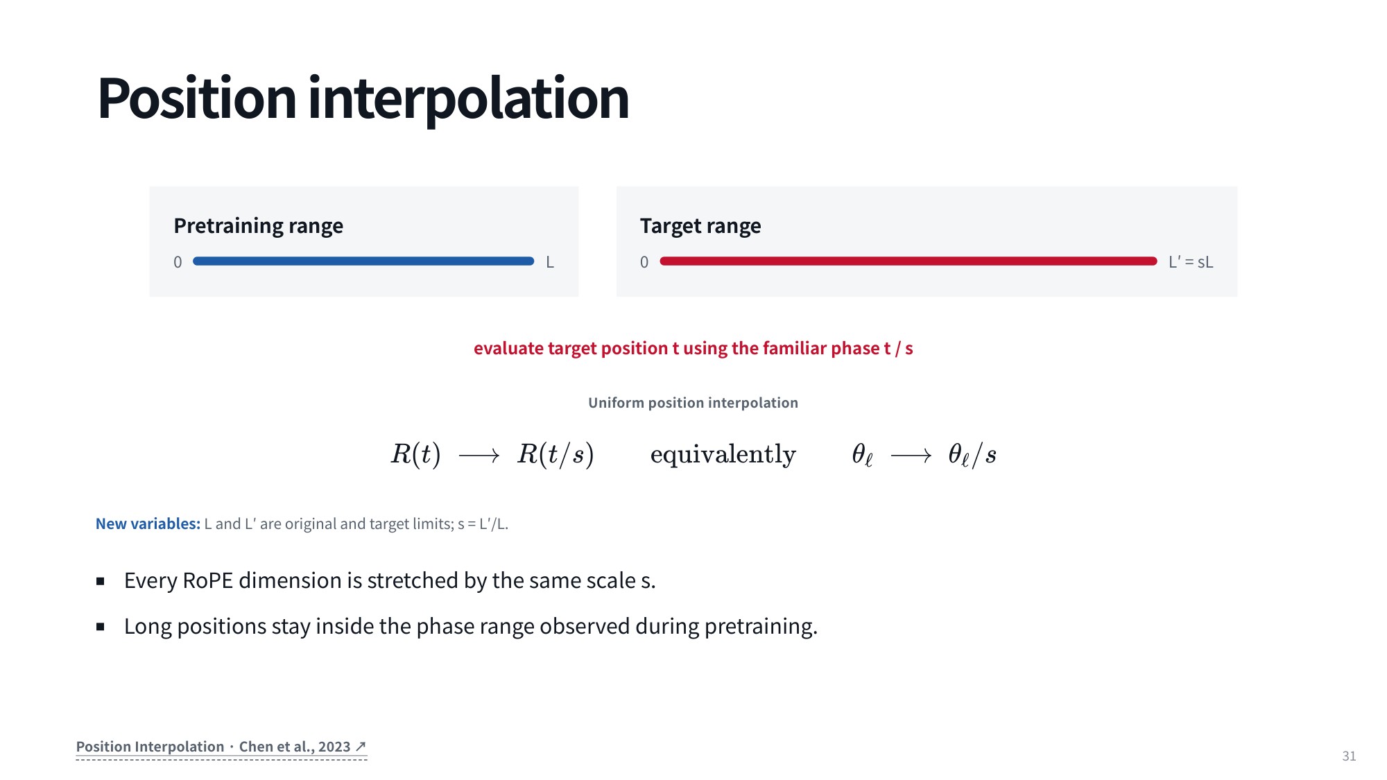
Fig 9. Position interpolation
Transforming the rotation operator uniformly and scaling down each base angle frequency compresses the whole target range ([0, L’]) into the pretrained interval ([0, L]), so the full target context window fits inside the phase dynamics seen during pretraining. The model never faces out-of-distribution phases, relative order is preserved across long contexts, and we get a clean baseline mechanism for handling longer sequences.
5. Frequency-Selective YaRN and Model Extension Paths
5.1 How YaRN Interpolates Frequencies
Suppose our architecture does keep positional encodings instead of dropping them. When we scale context length with Rotary Position Embedding (RoPE), plain position interpolation is a blunt instrument: it stretches every rotary frequency uniformly. That uniform stretch destroys the model’s ability to tell nearby tokens apart, blurring exactly the local relationships that carry syntax and grammar.
YaRN (Yet another RoPE extensioN method) fixes this. Rather than applying one scale factor (s) to every dimension, it interpolates selectively, adjusting each rotary dimension according to its wavelength.
[\theta’\ell = (1 – \gamma\ell)\frac{\theta_\ell}{s} + \gamma_\ell \theta_\ell, \quad 0 \le \gamma_\ell \le 1]
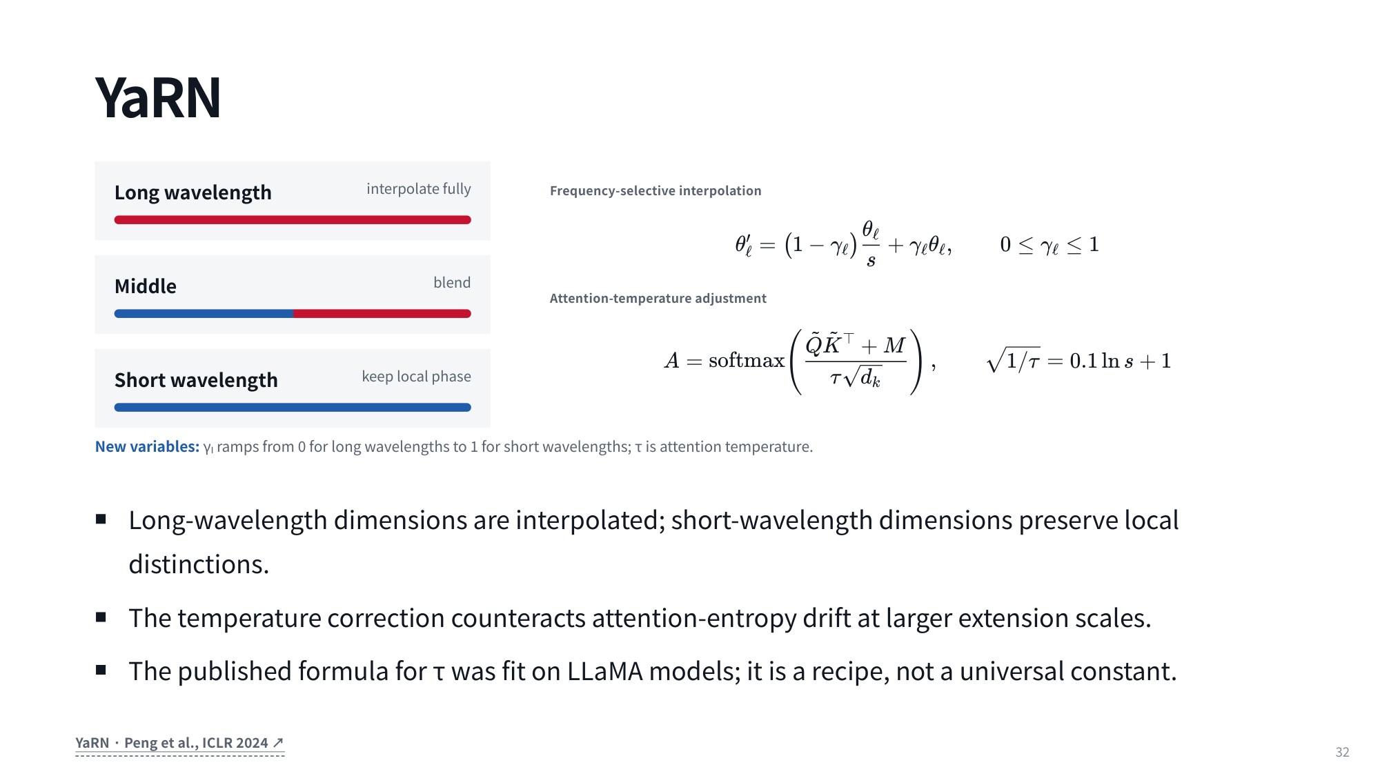
Fig 10. YaRN
The parameter (\gamma_\ell) is a ramp that moves smoothly from 0 for long wavelengths to 1 for short ones. High-frequency components with short wavelengths get (\gamma_\ell = 1), leaving the original rotation angle (\theta_\ell) untouched so adjacent tokens stay crisp and distinguishable to the attention heads. Low-frequency components with long wavelengths rarely complete a full period inside a short pre-training context, so they get (\gamma_\ell = 0) and are fully interpolated down to (\frac{\theta_\ell}{s}). Everything in between is blended.
Wavelength handling is only half the method. YaRN also adds an attention temperature (\tau) that re-normalizes how sharp the attention distribution stays as sequences grow. Without it, attending over far more positions pushes attention entropy up, diluting the weights until focused queries turn into washed-out averages.
Scaling the logits by (\tau), with (\sqrt{1/\tau} = 0.1 \ln s + 1), keeps the distributions calibrated at long context. One caveat worth remembering: that logarithmic formula was fit empirically on LLaMA models. It is an effective engineering recipe, not a universal constant, so expect to re-tune (\tau) on a different architecture.
[A = \mathrm{softmax}\left(\frac{\tilde{Q}\tilde{K}^{\top}}{\tau \sqrt{d_k}} + M\right), \quad \sqrt{1/\tau} = 0.1 \ln s + 1]
5.2 Positional Choices Across Models
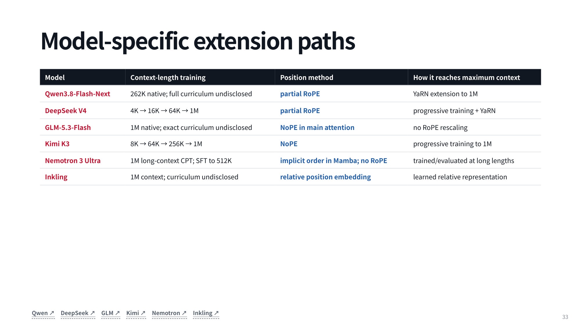
Fig 11. Model-specific extension paths
Compare the models side by side and the split is clear. Qwen3.8-Flash-Next and DeepSeek V4 use partial RoPE for token positions. GLM-5.3-Flash uses NoPE in its main attention, and Kimi K3 uses NoPE too, so no positional encodings at all. Nemotron 3 Ultra leans entirely on the implicit token order in Mamba with no RoPE, while Inkling uses a learned relative position embedding. Roughly half the field keeps some relative positional encoding and half drops explicit positions.
5.3 Adaptation Paths Across Architectures
The summary table lines up the context extension paths for Qwen3.8-Flash-Next, DeepSeek V4, GLM-5.3-Flash, Kimi K3, Nemotron 3 Ultra, and Inkling. For each it gives the context-length training regimen, the positional embedding strategy (partial RoPE, NoPE, implicit order in Mamba, relative position embeddings), and the mechanism used to reach the maximum context, such as YaRN extension or progressive training.
The takeaway is that context extension is not a one-size-fits-all problem. Whether a model uses partial rotary embeddings, no positions at all, or state-space ordering, stretching the context means aligning the math of the positional encoding with the multi-stage training pipeline. Progressive pre-training plus temperature-corrected frequency interpolation is what lets modern LLMs reach huge context horizons while keeping attention sharp and local token representations intact.
6. Context Parallelism and Distributed Training
6.1 Scaling Long-Context Training
If you ever train larger models yourself, one logistical detail eventually becomes unavoidable: context parallelism. Before getting there, it helps to recall the standard ways of spreading compute across machines. The usual baseline is data parallelism, and next to it sits the broader family of model parallelism.
Model parallelism comes in several varieties: expert parallelism, where different expert networks live on different physical machines; tensor parallelism, where weight matrices and parameter tensors are sliced across devices; and pipeline parallelism, where sequential layers are partitioned across devices.
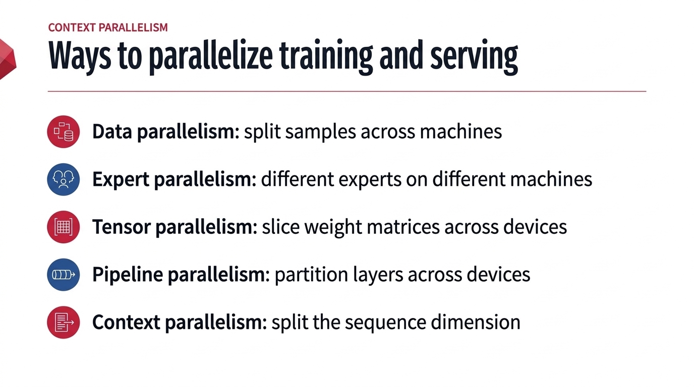
Fig 12. Ways to parallelize training and serving
Those paradigms split samples, parameters, or layers. Context parallelism splits something else, and it becomes critical precisely for agents, because training agents means training on very long contexts. In the CMU lecture, Neubig puts the threshold at roughly 32K tokens of context: above that, context parallelism becomes really important.
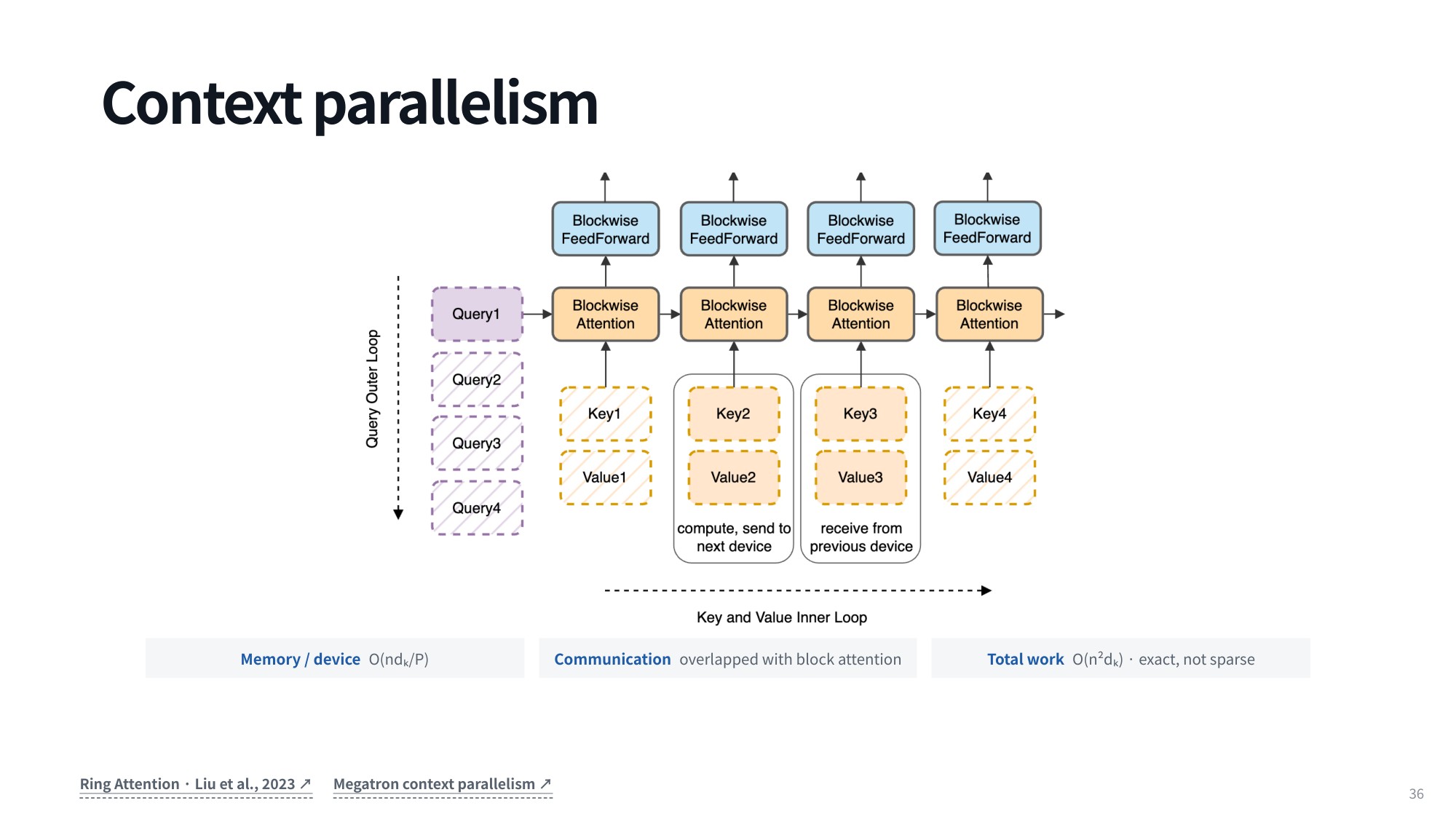
Fig 13. Context parallelism
The mechanism is to partition the sequence dimension itself. One device computes the keys and values for its slice of the context, sends them to the next device, which computes attention outputs for its partition, passes them along, and so on around the cluster.
The catch is that this is a large engineering burden to support. Systems engineers hit friction as soon as modeling researchers show up asking for their Kimi Delta Attention — wiring specialized attention mechanisms and recurrent operators into these distributed communication patterns adds real overhead.
6.2 Ring Attention and Megatron Overlapping
The good news is that standard attention, sliding window attention, and similar operations have efficient kernels that are comparatively easy to implement. Ring Attention and Megatron context parallelism overlap communication with computation so that keys and values circulate in a ring while each device computes its local attention blocks.
Because these setups follow familiar, well-supported execution paths, high-performance kernels are straightforward to obtain. The difficulty appears the moment you step outside them and are no longer running a standard attention operation — kernel implementation and execution get much harder to manage.
6.3 When the Kernel Does Not Exist Yet
The friction is concrete. Modeling teams want the newest recurrent layers such as Gated DeltaNet and Kimi Delta Attention, and infrastructure teams then have to write a context-parallel kernel for each one, verify correctness, and confirm that gradients flow through it.
In the CMU lecture, Graham Neubig describes trying to train a smaller Qwen model with context parallelism and finding that no context-parallel kernel for Gated DeltaNet existed anywhere. The choice was to implement it himself or drop context parallelism entirely, which matters as soon as training goes above roughly 32K tokens of context. The architectures themselves — sliding windows, linear attention, DeltaNet, KDA, sparse attention and MLA — are covered in LLM_log #030.
7. KV Caching Mechanics and Prefix Reuse
7.1 How Decoding Extends State in Multi-Turn Agents
Prompt and KV cache reuse matters whether you are implementing a language model or orchestrating agents in production. It pays to understand exactly what happens under the hood, so let’s trace the mechanics step by step.
A single agent call unfolds in three phases: an input, an output, and a tool result. The input holds things like system instructions and conversation messages. The output is the model’s response or its structured tool calls, which the execution environment then evaluates to produce a tool result.
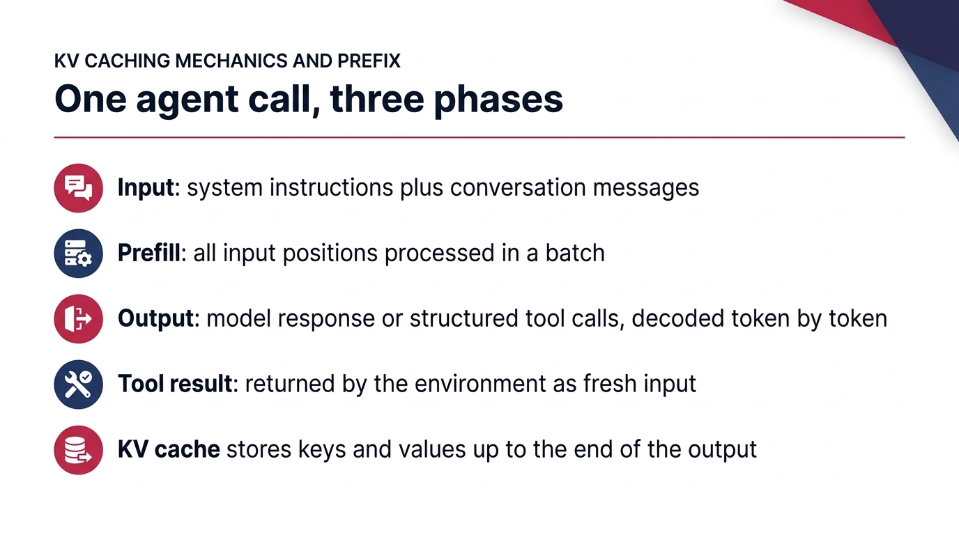
Fig 14. One agent call, three phases
Computing representations over the input sequence is prefill, and it runs efficiently as a batch. Generating the output switches to token-by-token decoding. In both phases we compute keys and values for every position up to the end of the generated output, and we store them in a cache instead of recomputing them later.
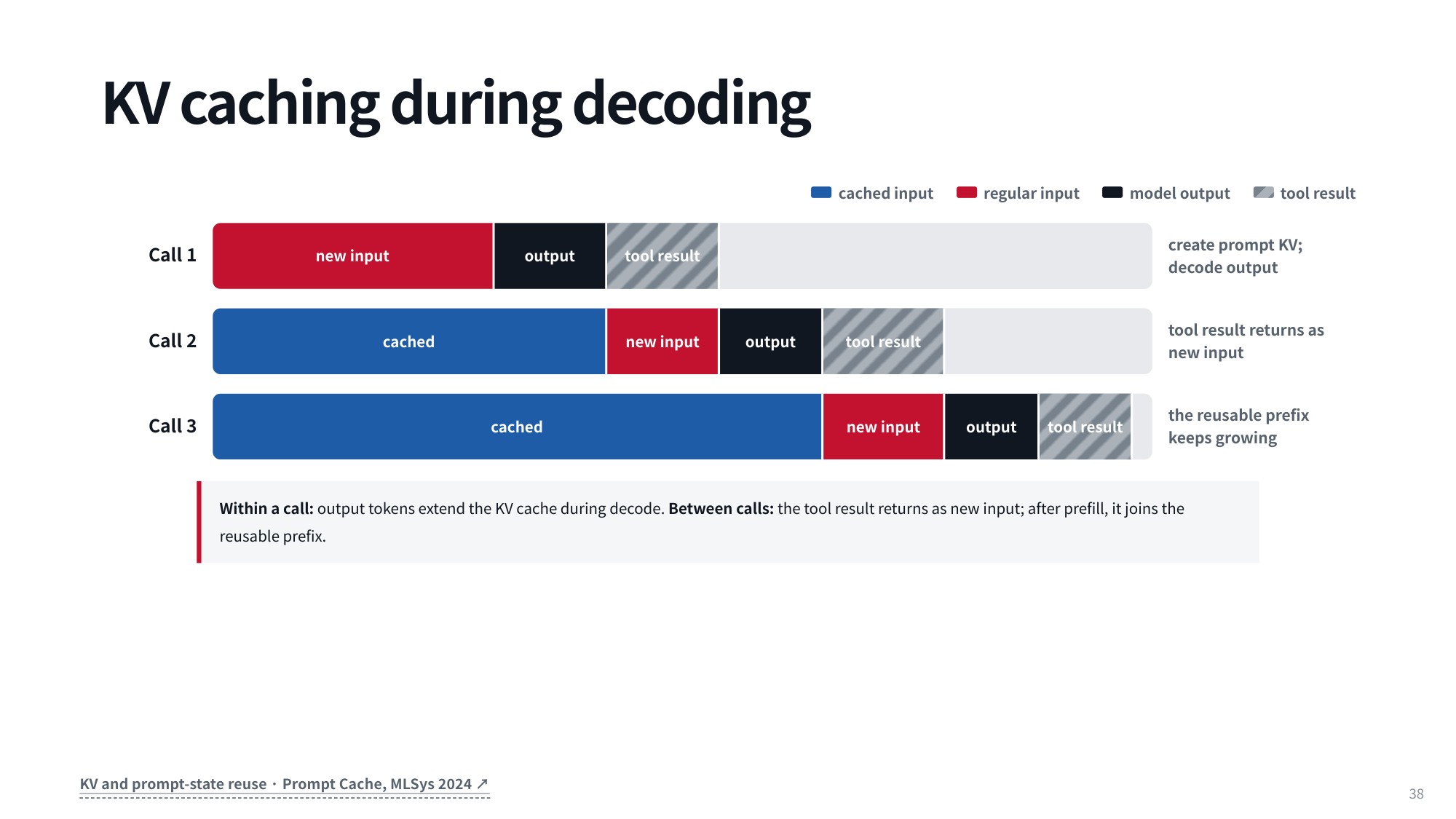
Fig 15. KV caching during decoding
The tool result comes back from an external environment, so the model has never computed anything over it: it enters as completely fresh input. In step two, that tool result is the new input, producing a new output and another tool result. We only prefill the new input and decode the new output tokens, reusing the existing cache for everything before it. The procedure repeats for the entire lifetime of the agent.
This looks harmless at steps one, two and three, but consider the scale later on. By step 50, assuming nothing has modified the historical output, the cached history is roughly 50 times larger than the new input and output processed in that step. Caching that state properly is where the savings come from.
7.2 Prefix Reuse During Generation
With prior states available, you never rerun the model over preceding context. You look up the stored outputs instead of redoing the matrix calculations over them. Retrieving precomputed values from memory rather than recalculating them makes extending generation dramatically cheaper.
7.3 Measured Gains from Cache Reuse
How large is the effect in practice? Published benchmarks plot the compute required across token lengths on several GPUs, with and without caching. For each hardware setup, shown in matching colors, the upper curve is the no-caching case and the lower curve of the same color is execution with caching enabled.
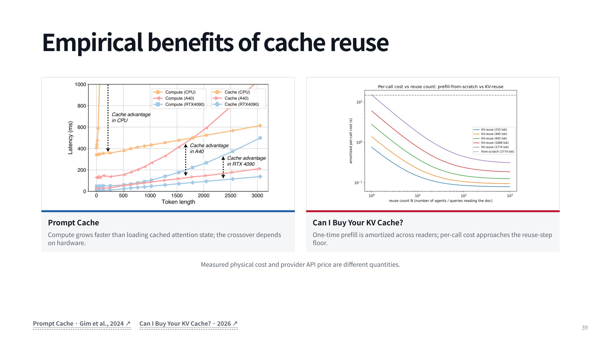
Fig 16. Empirical benefits of cache reuse
The critical takeaway appears as sequences get longer: the non-cached approach scales quadratically, while the cached approach stays mostly linear. In Transformer architectures, the feed-forward network is especially expensive in compute cost and parameter throughput. Skipping that computation entirely for every historical token is a massive win.
8. Paged Memory Allocation and Prefix Trees
8.1 PagedAttention and GPU Memory Management
Caching is cheap in principle, but the engineering difficulty starts with where the KV cache actually lives in physical memory. The two most popular open-source serving libraries, vLLM and SGLang, both grew out of innovations aimed at exactly that problem. vLLM has since become a general-purpose serving stack, but the algorithm that put it on the map was PagedAttention.
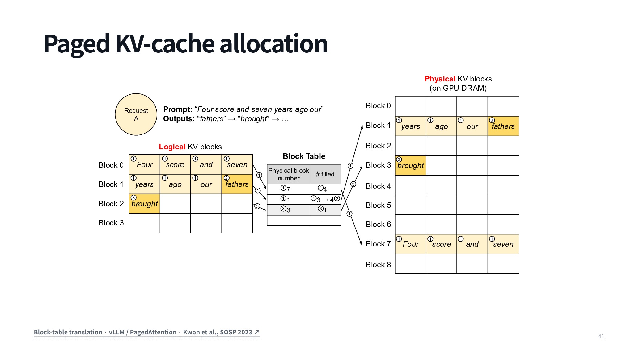
Fig 17. Paged KV-cache allocation
PagedAttention borrows directly from classical virtual memory paging in CPU operating systems. Instead of reserving one large contiguous chunk of GPU DRAM per sequence, it splits physical GPU memory into uniform blocks and decouples them from the sequence’s logical blocks.
So when attention runs over logical blocks (0), (1), and (2), the runtime can scatter them anywhere in physical memory — logical block (0) to physical block (7), logical block (1) to physical block (1), logical block (2) to physical block (3) — with an internal block table keeping track of the mapping.
That mapping is maintained throughout generation. Take a prompt like “Four score and seven years ago our”: its tokens fill the first logical blocks, and as output tokens arrive step by step — “fathers” (\to) “brought” (\to) and onward — they fill the current block. When a block fills up, a new physical block is allocated on demand and registered in the table. This avoids fragmentation and removes the need to pre-allocate worst-case memory for every sequence.
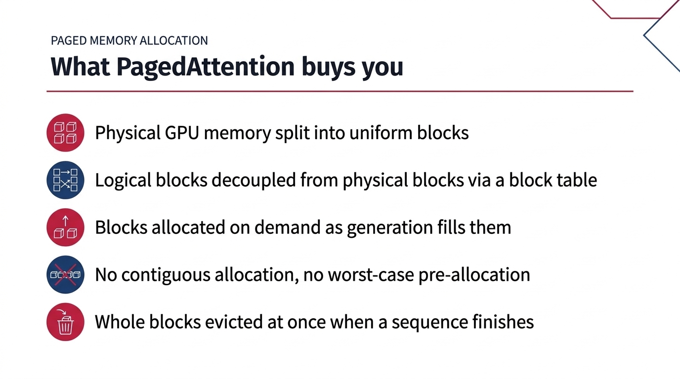
Fig 18. What PagedAttention buys you
8.2 Paged Allocation for Parallel Serving
The runtime keeps an index into each of these blocks as generation proceeds. The real motivation for this design is concurrency: serving many sequences in parallel. When a sequence finishes, the runtime evicts it cleanly, and evicting whole blocks at once makes the bookkeeping far more efficient.
This is one of the breakthroughs that made high-throughput parallel serving work at scale. The bad news for us as end users is that our pricing does not change, however good a provider gets at cache eviction or request routing. And while PagedAttention handles dynamic memory blocks inside a running instance, reusing shared prefixes across requests needs a different structure entirely.
8.3 RadixAttention and Prefix Sharing
vLLM attacked physical memory fragmentation; SGLang was built around RadixAttention, which targets reuse of outputs already computed and stored in the cache. It organizes the cache as a radix tree and uses it to look up token prefixes that have already been processed by past and concurrent requests.
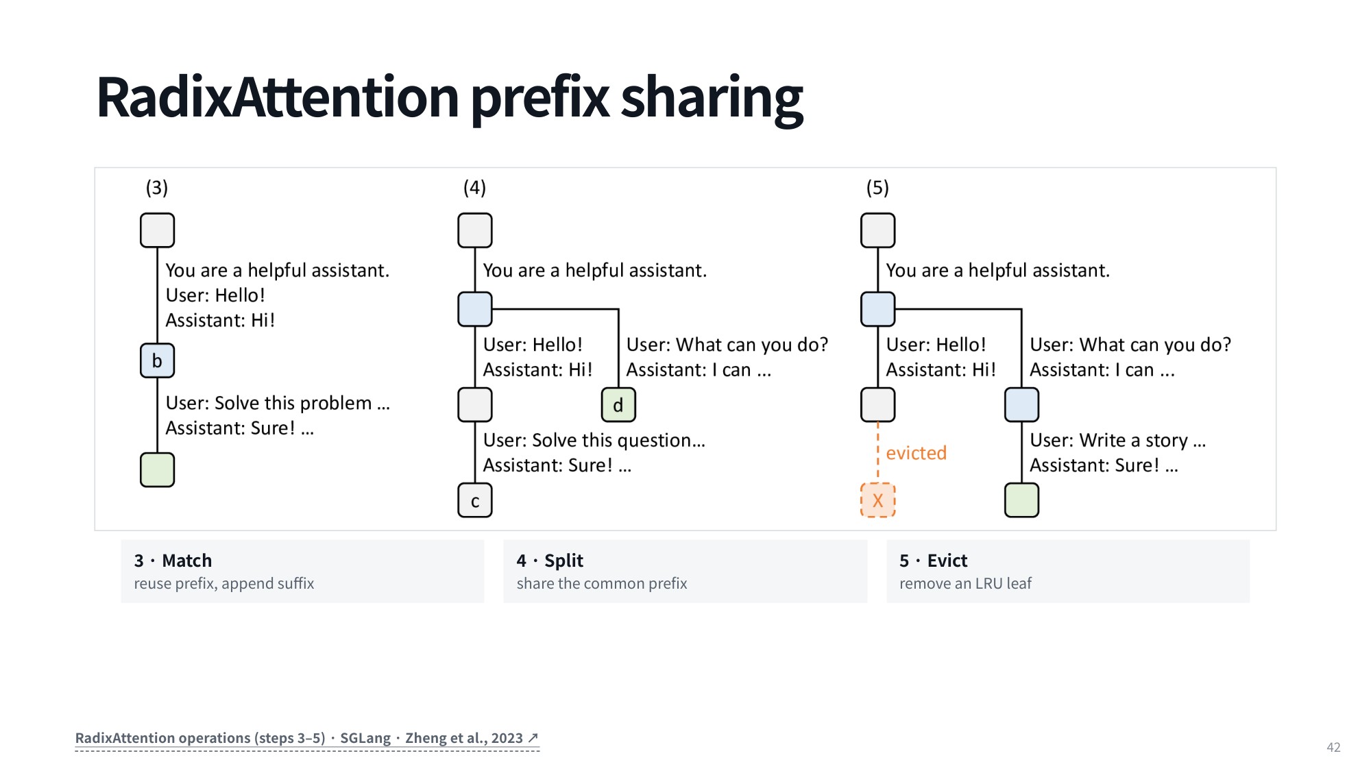
Fig 19. RadixAttention prefix sharing
RadixAttention was originally designed around multi-turn chatbots like ChatGPT, where a user starts a conversation and keeps extending it. The system caches part of the already-generated history and skips redundant prefill computation on each turn.
As the CMU lecture points out, prefix caching now matters far more for agentic systems. Agent trajectories produce much longer conversations and call the model far more often, so frequent prefix lookups become essential to keeping the system efficient and responsive.
9. Cache-Aware Routing and Serving Infrastructure Metrics
9.1 Cache-Aware Routing Across Serving Nodes
Scaling a serving stack across many machines introduces a problem that newer versions of SGLang handle directly. Picture a data center running a fleet of 64 nodes, 128 nodes, or more: route incoming requests naively across them and efficiency collapses.
The goal for every new request is to send it to the worker that already holds the best KV cache state for that prompt. Cache-aware routing steers traffic so the worker with the highest KV cache match handles the request, with minimal redundant prefill computation.
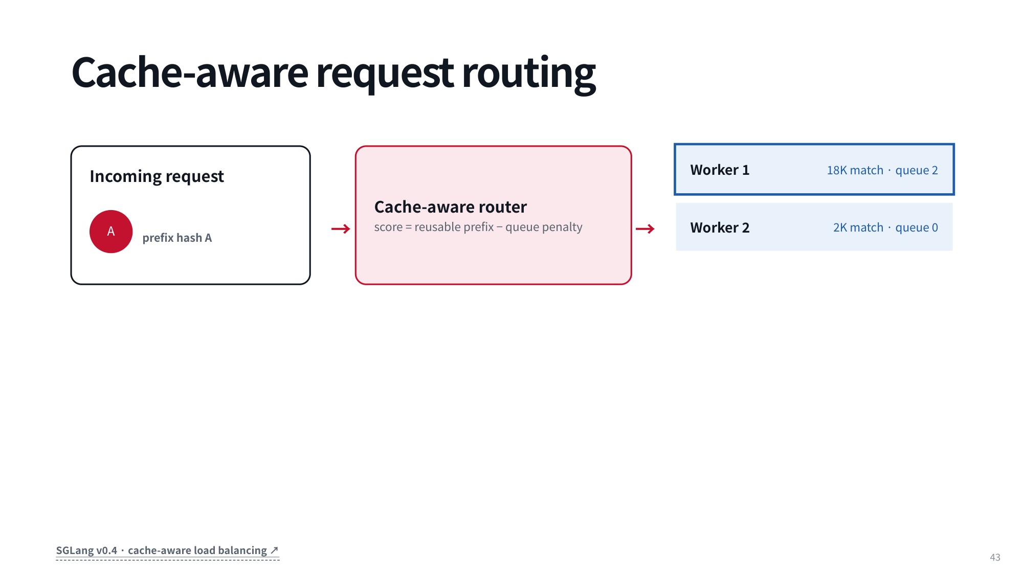
Fig 20. Cache-aware request routing
In the CMU lecture, Graham Neubig draws his serving statistics from OpenRouter, which publishes an enormous amount of operational data that illustrates these phenomena well. One thing the public metrics do not reveal is whether providers run a layered cache: a fast tier in GPU memory backed by a slower tier on host CPU memory, secondary storage, or disk. That remains an open question.
GPU-to-CPU offloading, on the other hand, is widespread. Offloading KV cache states to host memory is standard practice across the industry because GPU high-bandwidth memory is so precious, and this hierarchical memory management is what keeps serving capacity high and infrastructure costs under control.
How do open-source libraries compare to proprietary stacks? Probably not quite as sophisticated. The inference providers competing on OpenRouter live or die on serving performance, so even when they start from off-the-shelf open-source libraries, they build custom features on top. Their internal caching mechanisms are likely a step ahead of what you get out of the box.
9.2 Cluster-Level Cache Routing
At the cluster level, incoming requests are tagged by their prefix hashes and evaluated by a cache-aware router before being forwarded to distributed worker nodes.
To pick the best node, the router scores candidate workers explicitly:
[\text{score} = \text{reusable prefix} – \text{queue penalty}]
Each request goes to the worker that best balances prefix cache reuse against queue overload. That balance directly shapes time-to-first-token latency and overall system throughput.
9.3 Latency, Throughput, and Provider Benchmarks
How do these routing differences show up in production? OpenRouter tracks public benchmarks across the hosting providers serving models like GLM-5.2, including provider rankings by observed cache hit rate.
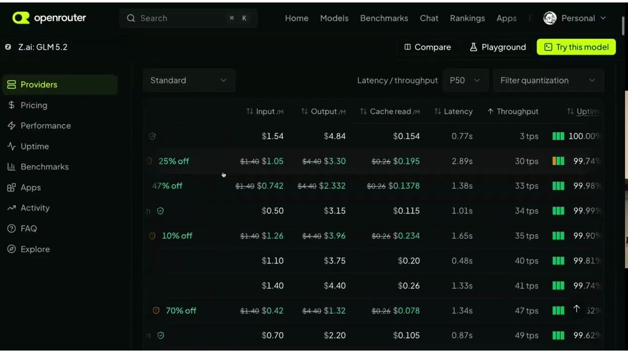
Fig 21. Cache hit rate, latency and throughput across GLM-5.2 providers on OpenRouter
The numbers speak for themselves. Mistral has the worst cache hit rate among the tracked options, while Alibaba Cloud, Decart, and SiliconFlow achieve noticeably higher rates on the same workloads.
A lower cache hit rate is not automatically an indictment of a provider’s infrastructure. It often just reflects the workloads and traffic patterns hitting that endpoint. Still, two technical factors dictate the rate you actually get: the efficiency of the provider’s cache routing architecture, and how aggressively they run cache eviction.
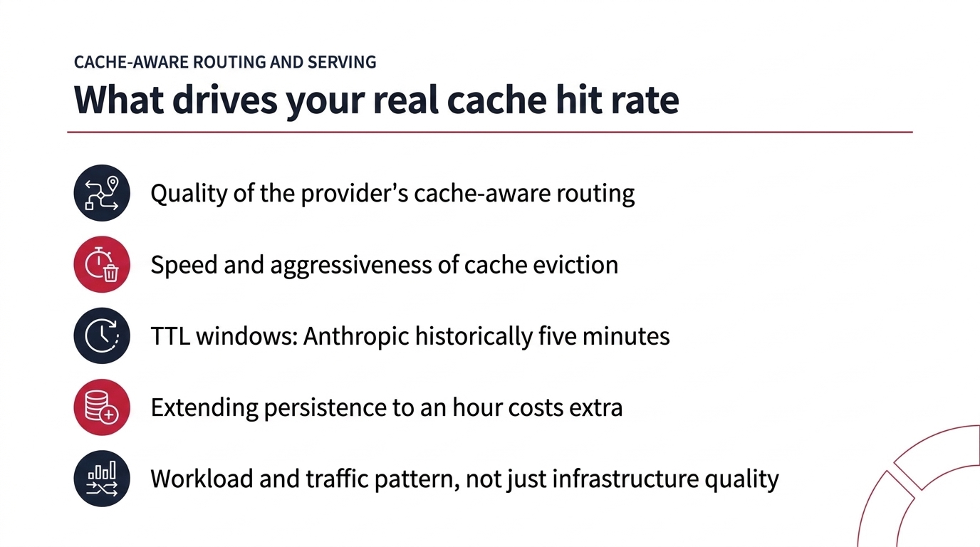
Fig 22. What drives your real cache hit rate
No provider can store your context indefinitely, because idle KV caches tie up expensive high-bandwidth memory. Eviction therefore runs on strict time-to-live (TTL) thresholds. Anthropic, for example, historically maintained a five-minute window: an active back-and-forth conversation stays resident, but a longer pause gets your cached state evicted. Some platforms now offer cache persistence up to an hour, usually at an added cost. What that eviction behavior does to your bill is the subject of the next section.
10. Prefix Caching Economics and API Pricing Models
10.1 What Prefix Caching Saves
On OpenRouter, providers such as Mistral, Baseten, and Sail Research list the input price per million tokens, the output price per million tokens, the cache read cost, and latency and throughput statistics side by side. That layout makes the economic impact of prefix caching easy to read off directly.
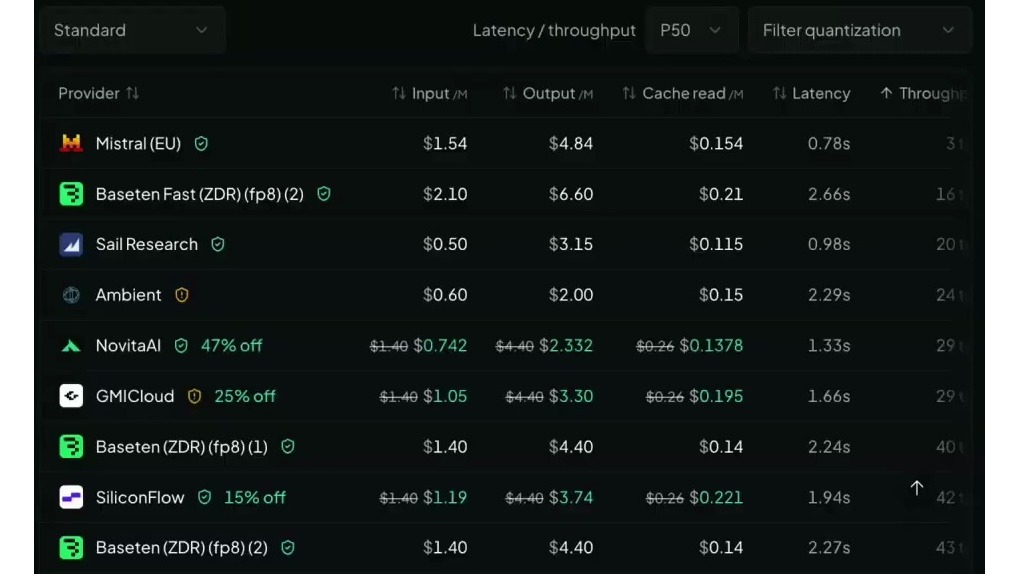
Fig 23. Provider pricing and latency statistics for models on OpenRouter
10.2 Cached-Token Pricing and Agent Costs
The same effect shows up in what you pay to run an agent. The CMU lecture pulls these figures from official pricing sheets, and across the board, including commercial models, cached tokens cost roughly one tenth of uncached tokens. With a discount that steep, you need to know whether your tokens are actually hitting the cache; if they are not, running agents gets expensive fast.
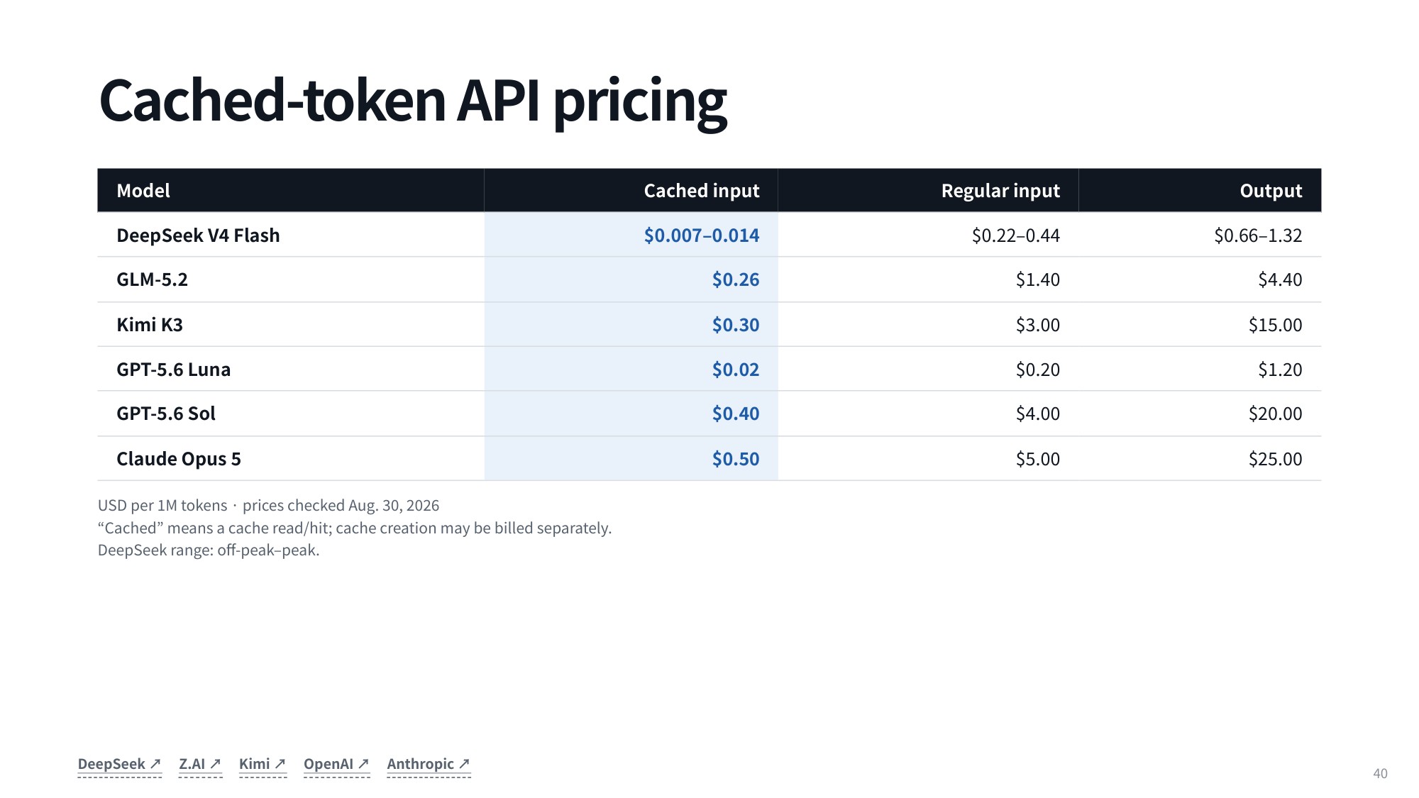
Fig 24. Cached-token API pricing
So what counts as a good cache hit rate? Practitioner estimates usually land between 80 and 90 percent, with some teams pushing past 95 percent. Graham Neubig considers 90 to 95 percent a comfortable range. Below that, your system still runs, but you are losing money somewhere, because the vast majority of your tokens should be cacheable.
One more detail in these tables: output tokens tend to cost five times more than regular input tokens. Combined with the caching discount, that is roughly a 50x gap between output tokens and cached input tokens, which reflects how much providers save when they serve a request straight from cache.
The practical consequence is to be frugal about how much you switch between models or contexts when cost matters. And since the price is fixed on your side, you can end up paying full price simply because the provider evicted your context too quickly, which feels a little unfair. Given these ratios across commercial offerings, the real question is how we manage caching deliberately.
11. Prompt Engineering for Prefix Cache Preservation
11.1 Prompt Layout for Maximum Prefix Reuse
Even if you never deploy a model or touch serving infrastructure, KV caching shapes how you should design an agent harness. The rule to keep in mind is strict: prompt caching only works when the entire prefix is byte-for-byte identical across requests. Several design ideas that look sensible on paper turn out to be bad purely because they invalidate that prefix.
The one thing you must never do is change your system message on every execution step. Mutating the very beginning of the prompt leaves the engine with no cacheable prefix at all, which wipes out prompt caching for the whole run.
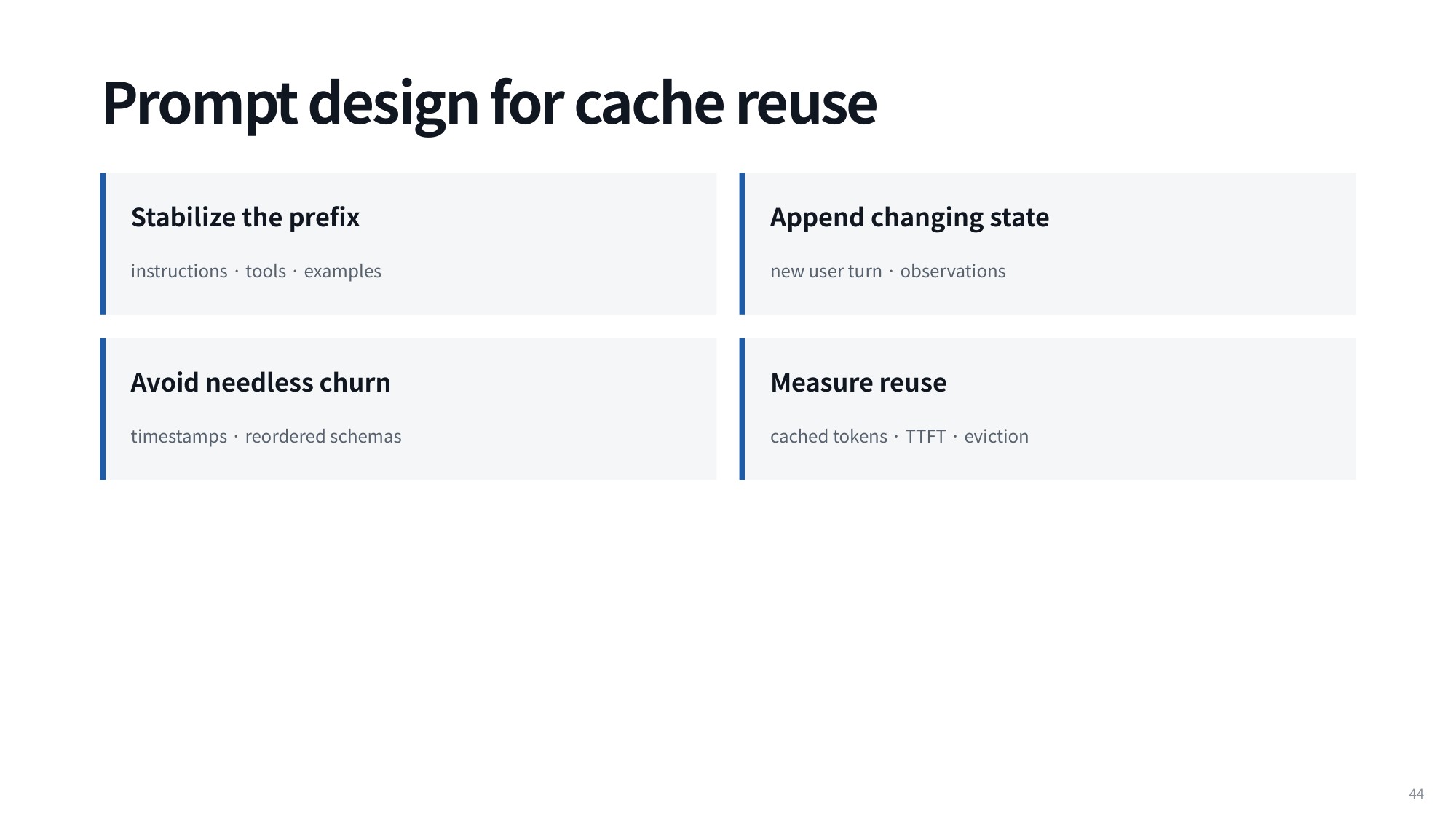
Fig 25. Prompt design for cache reuse
11.2 Avoiding Prefix Churn
A tempting example: append the current time and date to the system message so the agent always knows what time it is. Don’t. The timestamp changes on every step, so the system message changes too, and the cache breaks from token zero onward.
If the model genuinely needs temporal information, put it at the tail of the prompt instead — in the final user message or in the latest tool call result. Tool definitions can be changed mid-conversation, but tools live in the stable prefix, and any edit there invalidates everything after it. As the lecture puts it: stabilize the prefix of instructions, tools and examples, and avoid needless churn such as timestamps or reordered schemas.
Another popular idea is per-step model routing. You inspect an upcoming step, decide it needs a heavy, capable model, run that one step on the expensive frontier model, then drop back to a cheaper model for the next three steps to save money.
The catch is that bouncing between models loses your cache state on each of them. The next call to the expensive model pays the full 10x cost again, which cancels out the savings you were chasing.
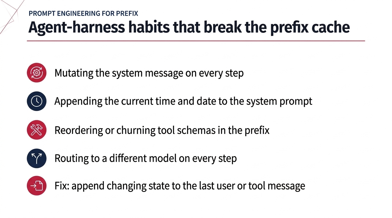
Fig 26. Agent-harness habits that break the prefix cache
12. Context Compaction as Agent State Estimation
12.1 Compression as State Estimation
For agents that run over long trajectories, history compression is cleaner to reason about as state estimation than as an ad hoc truncation heuristic. We treat the interaction history as an uncompressed sequence (H_t) and map it into a compact working state (\hat{s}_t) using an explicit compactor (\mathcal{C}_B), which processes the full conversational and environmental history under a token budget (B). That bounded representation is what the model actually conditions on for every subsequent inference step.
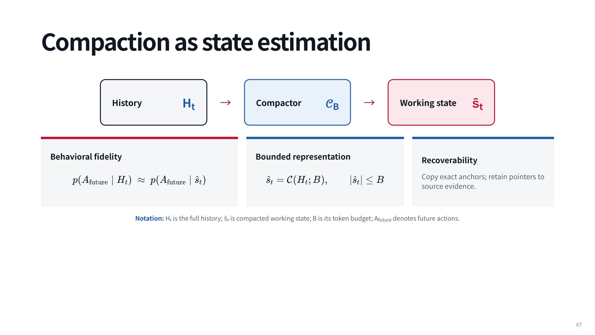
Fig 27. Compaction as state estimation
The objective is behavioral fidelity: preserving the agent’s decision distribution over future actions (A_{\text{future}}). The compacted state must act as a sufficient statistic of the full history, satisfying (p(A_{\text{future}} \mid H_t) \approx p(A_{\text{future}} \mid \hat{s}_t)). When that holds, conditioning on (\hat{s}_t) induces virtually the same policy as conditioning on the complete history, so downstream execution does not degrade even under strict capacity limits.
[\hat{s}_t = \mathcal{C}(H_t; B), \quad |\hat{s}_t| \le B]
Operationally, a compactor rests on three pillars: behavioral fidelity, bounded representation, and recoverability. Bounded representation enforces that (|\hat{s}_t|) never exceeds (B), preventing memory exhaustion and context window overflow. Recoverability demands that critical elements dropped from active working memory stay accessible or reconstructible when a later subtask needs details that were omitted.
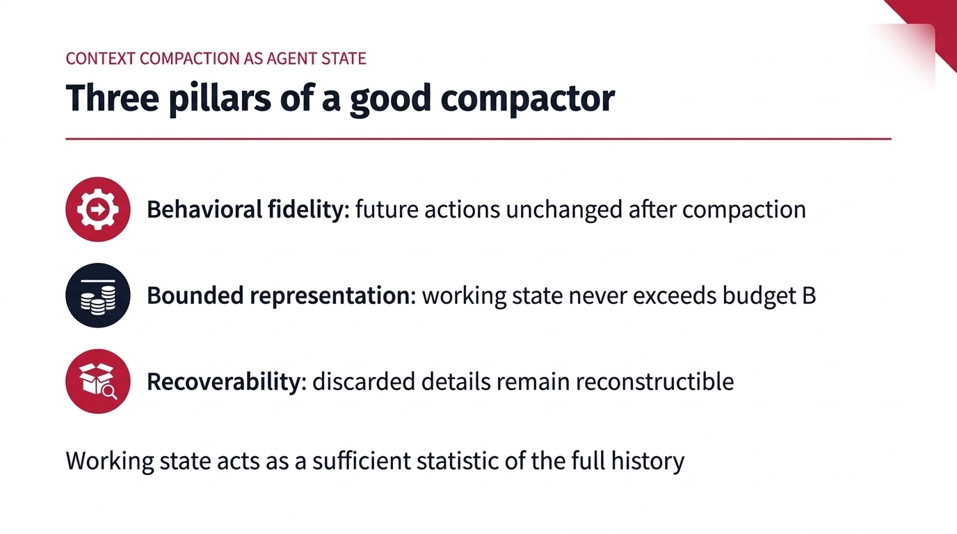
Fig 28. Three pillars of a good compactor
12.2 Compressing Observations and Actions
In real agent workflows this means compressing verbose observations and tool actions. The uncompacted trajectory holds detailed CI job logs, long terminal outputs, and execution commands piled up over time. Compaction crushes that down to the essential core of what happened: the verified goal and the key evidence needed for the next steps, with the noisy intermediate output dropped.
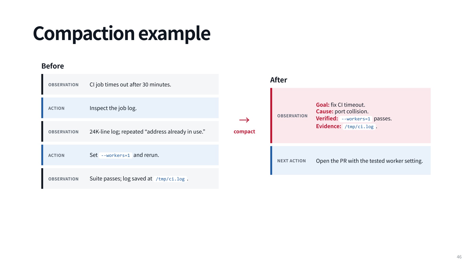
Fig 29. Compaction example
Why are practitioners often reluctant to enable it? Because a bad compaction makes the agent forget things. It gets confused, starts doing something entirely different, and may even delete your file system. Framing compaction as building a representation under which the future action sequence stays predictable is what guards against that: you take the history, compact it, get a working state, and expect the future action sequence to be the same, similar, or even better than before.
All of this runs against a hard constraint. The state must stay strictly bounded, small enough to keep working without exhausting the context budget or adding unnecessary inference overhead.
13. Context Compaction Policies, Anchors, and Repeated Compaction Drift
13.1 Anchors, Checkpoints, Recent Tail and Evidence Store
What actually survives context compaction? The most reliable pattern starts with preserving anchors: the first instructions, the system prompt, and the primary goal the user stated at the beginning of the session. Those set the objective, the boundaries, and the constraints that govern every downstream turn.
In the CMU lecture, Graham Neubig reports that one of the most common complaints about agents is that they lose the instructions given at the very start. That is usually a design bug in the harness rather than a model failure: naive systems prune sequentially from the front of the prompt, while a well-built harness protects the opening turn from deletion. Truncation is hard to avoid entirely under tight window limits, but dropping your starting instructions is almost always catastrophic.
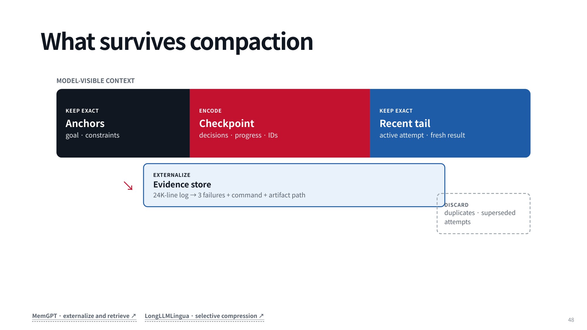
Fig 30. What survives compaction
Between the anchors and the current step sits the sprawling middle history, which cannot simply be thrown away. It has to be transformed instead: we encode it into structured checkpoints that capture architectural decisions, cumulative progress, and essential identifiers, then reinsert those into the active prompt.
The recent tail — the latest actions, the active attempt, the most recent execution outputs — stays raw and intact. That gives the agent operational continuity, so it can read the latest tool output, catch an error, and adjust its next step without perceptual lag.
Everything else can be externalized into a dedicated evidence store. Fully structured evidence stores are not yet standard across frameworks, but nearly all CLI coding agents already persist their conversation history and terminal logs to disk. If you know where those logs live, you can ask the agent to read its own history back and recover terminal output or error messages lost during compaction. Offloading verbose traces, raw tool logs, and superseded attempts lets the system drop duplicate or obsolete tokens from the prompt while keeping a verifiable audit trail for later retrieval.
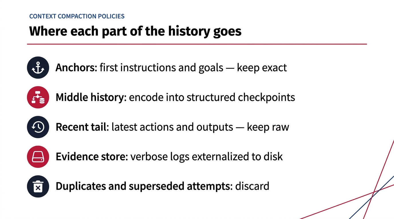
Fig 31. Where each part of the history goes
13.2 Trigger, Select, Replace, Recover
Turning these principles into a production system starts with the trigger mechanism. The common case is an automated token threshold: you decide to use at most 200k tokens, and the moment the prompt crosses that boundary, compaction fires.
Compaction can also be forced by the model provider as a hard ceiling on context tokens. Beyond automatic thresholds, good harnesses support manual requests — many coding agents expose a /compact command so the user can compress context on demand in the middle of a heavy debugging session.
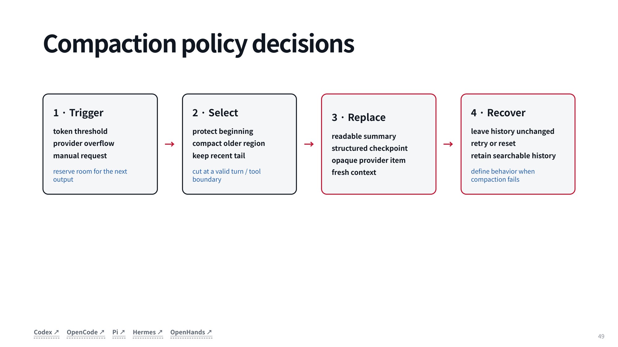
Fig 32. Compaction policy decisions
Once triggered, the policy must select which regions to alter. The standard approach protects the anchors at the front, preserves the recent tail, and isolates the older intermediate history for compaction.
That older material is then replaced with a condensed summary. Some systems use a structured summary produced by a dedicated tool call that mandates specific fields; others generate unconstrained free text.
Some providers (Neubig thinks possibly only OpenAI) compact the selected history into an opaque, encrypted state that cannot be inspected, which keeps outsiders from reverse-engineering their compaction algorithm. A complete policy also needs a recovery mechanism to pull externalized evidence back from disk. But applying these replacement steps over and over across a long session opens the door to serious information loss.
13.3 Repeated Compaction Drift
That compounding loss is repeated compaction drift. A single compaction pass usually preserves the critical state with no visible degradation. Compact repeatedly over a long trajectory, though, and each pass sheds a little more information until the agent drifts off the rails.
Formally, repeated compaction is recursive state estimation:
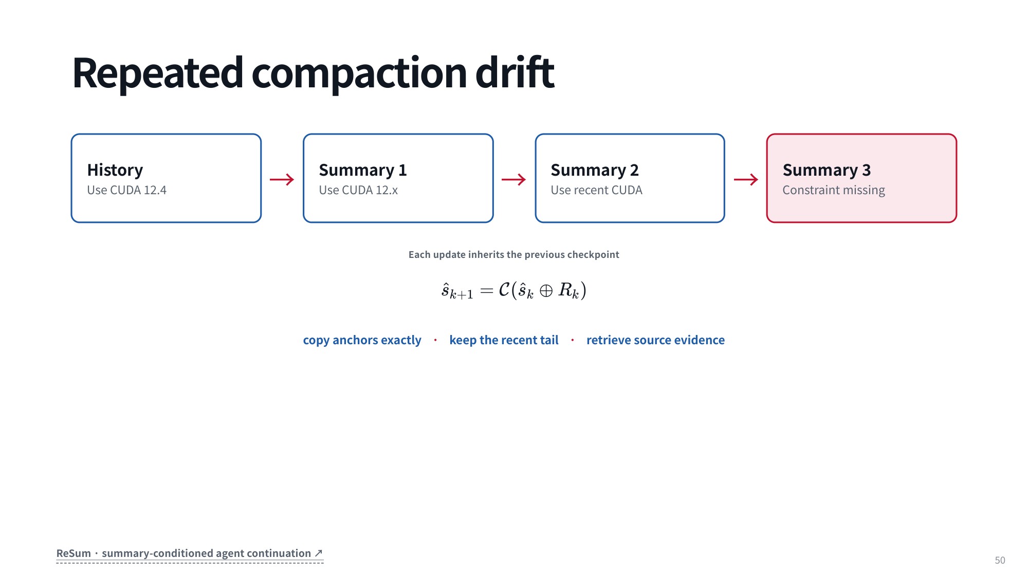
Fig 33. Repeated compaction drift
[\hat{s}_{k+1} = \mathcal{C}(\hat{s}_k \oplus R_k)]
The updated summary state (\hat{s}_{k+1}) comes from applying the compaction function (\mathcal{C}) to the prior summary (\hat{s}_k) concatenated with newly accumulated execution history (R_k). Across cycles, fine-grained detail dilutes.
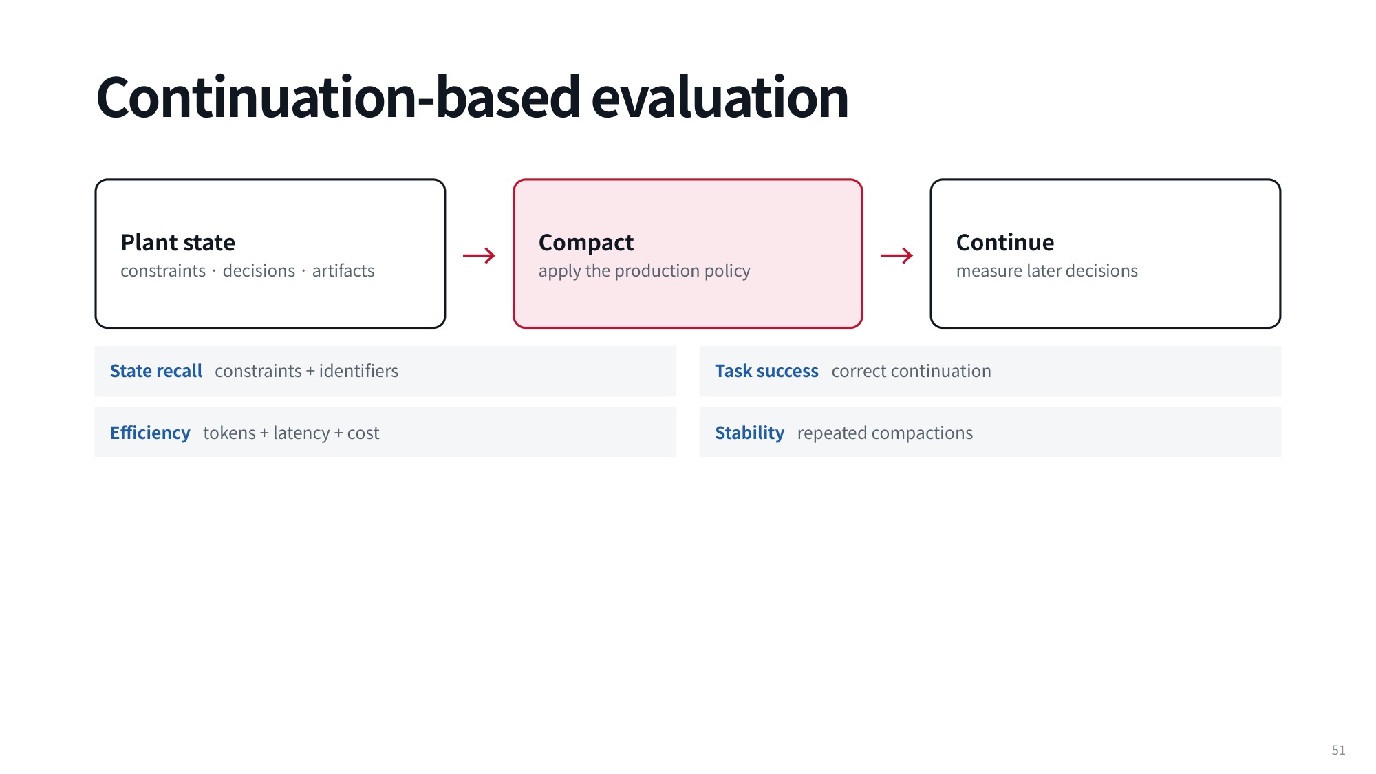
Fig 34. Continuation-based evaluation
The usual way to evaluate these algorithms is to sweep compaction strategies across downstream agent benchmarks — and the lecture offers a cautionary tale about exactly that. Early in OpenHands development, Neubig’s team built what was likely one of the first production-grade compaction systems, called compression at the time, and spent about a month benchmarking it against SWE-bench, the premier software engineering agent benchmark. The results looked excellent: large token savings with no drop in success rate.
Deployed live, the same policy immediately produced comical failures. The agent forgot it had already submitted a pull request to GitHub, opened another one on every compaction event, and ended up with five duplicate pull requests for the same functionality. It also erased user instructions issued midway through an interaction.
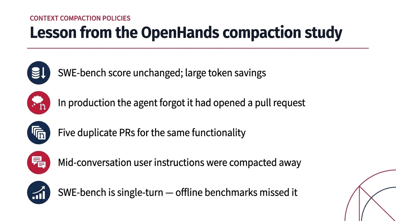
Fig 35. Lesson from the OpenHands compaction study
The cause was the benchmark itself. SWE-bench measures single-turn scenarios driven by one user prompt, so it could never reveal that the algorithm was compacting away mid-conversation feedback. Offline benchmarks are not enough unless they cover every realistic usage pattern, and testing in the wild remains essential. Agent loops grow fast, and the inference bottlenecks they create have to be managed through a balance of architectural innovation, efficient context compaction, and principled caching.
14. The Long-Context System Stack Across Agent Architectures
Everything we have covered stacks into five layers, and naming them explicitly helps: each layer answers a bottleneck created by the one above it.
1. Growth. Agent loops grow fast. The history before call (t) grows linearly, but the total input processed across the whole trajectory grows quadratically. That is why per-call inputs of 6K, 11K, 16K, 21K and 26K tokens already add up to 80K processed tokens by the fifth call.
2. Inference. That growth turns straight into inference pressure: prefill cost and time-to-first-token climb with prompt length, decode is sequential and memory-bandwidth-bound, and the KV cache grows with every position.
3. Architecture. Part of the efficiency problem is solved inside the model: sliding-window and hybrid local/global layers, linear and gated-delta recurrences, sparse attention, and KV compression such as grouped-query and multi-head latent attention. With these, a model can realistically handle up to a million tokens.
4. Caching. Prompt and KV caching handle the rest at the serving level. PagedAttention, RadixAttention and cache-aware routing make repeated agent prefixes cheap, and cached tokens typically cost about one tenth of uncached ones. Stable prefixes avoid repeated prefill, but they do not shrink the visible history.
5. Compaction. Once context grows past what we can practically handle, compaction takes over: crush the previous history down to its essence under a token budget, then continue from that bounded state.
Subagents are another way to keep each agent’s window small; the course covers them in a later lecture.
15. Summary
Ultra-long context is not one trick but a stack of coordinated decisions. Training is staged: short pretraining on standard document lengths, then continued adaptation on mixtures rich in codebases, scientific papers, and agent trajectories.
At the representation layer you have two options. Either stretch Rotary Position Embeddings with frequency-selective methods like YaRN, or drop explicit position coordinates entirely and let causal masking carry order, as NoPE does.
At the systems layer, throughput comes from serving and prefix caching. PagedAttention removes GPU physical memory fragmentation, RadixAttention keeps reusable prompt prefixes in radix tree structures, and cache-aware routing balances prefix hit rates against queue latency across multi-node deployments.
Since cached tokens are heavily discounted across commercial APIs, an agent harness has to guard against prefix invalidation — which means no dynamic mutations in early system instructions.
And when a run outgrows even a well-cached window, context compaction takes over as bounded state estimation: protect the instruction anchors at the prompt origin, keep the raw execution tail for operational continuity, and externalize intermediate traces to persistent storage so behavior survives a hard capacity limit.
Where to go next? The architectural half of this story — Multi-Head Latent Attention, hybrid sequence layers, and the rest of the KV-cache footprint work — is covered in LLM_log #030, the first half of Graham Neubig’s CMU lecture. Subagents are the other obvious way to manage context; the course returns to them in a later lecture, while the next session covers skills and memory.
Source
Lecture: Context Management for Long-Context Agents by Graham Neubig, Carnegie Mellon University.
Course: CMU 11-768 AI Agents (Fall 2026), Lecture 3, second half. The first half is covered in LLM_log #030.
Video: YouTube. Slides: PDF. Course page: cmu-agents.com.
Further reading referenced in the lecture:
- RoFormer (RoPE) — Su et al., 2021; NoPE — Kazemnejad et al., NeurIPS 2023
- Position Interpolation — Chen et al., 2023; YaRN — Peng et al., ICLR 2024
- Ring Attention — Liu et al., 2023; Megatron context parallelism
- Prompt Cache — Gim et al., MLSys 2024; Can I Buy Your KV Cache? — 2026
- PagedAttention / vLLM — Kwon et al., SOSP 2023; SGLang / RadixAttention — Zheng et al., 2023; SGLang v0.4 cache-aware routing
- MemGPT — Packer et al., 2023; LongLLMLingua — ACL 2024; ReSum — 2025
- Agent harnesses compared: Codex, OpenCode, Pi, Hermes, OpenHands
dataHacker.rs — LLM_log #031: Long Context in Practice — Training Recipes (RoPE, YaRN, NoPE), KV and Prompt Caching, and Context Compaction. By Vladimir Matic.