---

Highlights:

Stable Diffusion doesn’t paint an image in one shot — it sculpts one from static, guided by your words. In this post we disassemble the entire machine. We start with the VAE that compresses pixels into a tractable latent space, walk through the forward and reverse diffusion processes, open up the UNet to see how cross-attention physically connects text tokens to spatial regions, and finish with the complete Latent Diffusion architecture diagram that ties every piece together. By the end, you will be able to trace a single forward pass — from a text prompt and a seed of Gaussian noise to a generated 512×512 image — and explain exactly what happens at every tensor boundary. So let’s begin!

Tutorial Overview:

1. The Generative Model Landscape
2. DDPM: Forward and Reverse Markov Chains
3. The VAE — A Neural JPEG Compressor
4. VAE Quality Proof: Original vs. Reconstruction
5. Forward Diffusion in Latent Space
6. The Complete Forward + Reverse Process
7. Single Denoising Step — The Core Subtraction
8. Progressive Denoising — Image Emerges from Noise
9. The Three Components of Stable Diffusion
10. The Pipeline with Tensor Dimensions
11. CLIP Training: Three Steps to a Shared Embedding Space
12. UNet: Three Inputs, One Output
13. Inside the UNet — ResNet + Cross-Attention
14. The UNet Training Loop
15. Training Dataset Structure
16. Conditional Generation on MNIST
17. Classifier-Free Guidance
18. LDM Complete Architecture
19. The Full Inference Pipeline
20. LDM Architecture — QKV Cross-Attention Focus
21. Summary

---

1. The Generative Model Landscape

Before we build Stable Diffusion, let’s orient ourselves. The generative model landscape is crowded, but fundamentally, every model here is trying to solve the exact same mathematical problem: mapping a simple, sampleable distribution (like a standard Gaussian \(\mathbf{z} \sim \mathbf{N}(0, I)\)) to the impossibly complex distribution of natural images \(p(\mathbf{x})\).

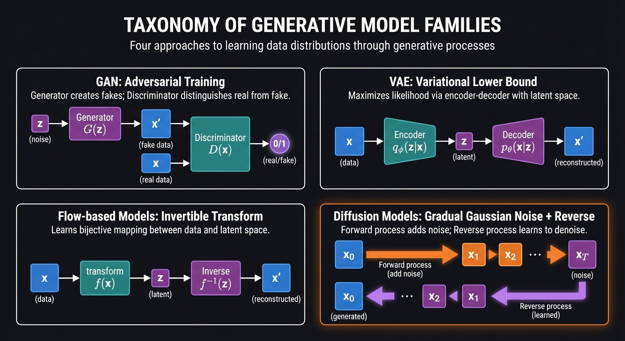
Four families have emerged, each with a radically different strategy:

• GANs learn this mapping implicitly through an adversarial game — a counterfeiter vs. police dynamic — bypassing density estimation entirely.
• VAEs act as a “neural JPEG,” forcing data through a low-dimensional bottleneck and optimizing a variational lower bound on the log-likelihood.
• Flow models use strict mathematical bijectivity to guarantee exact reconstruction, but at the cost of constrained, carefully designed architectures.
• Diffusion models break from the single-pass paradigm. Instead of mapping \(\mathbf{z}\) to \(\mathbf{x}\) in one leap, they define a Markov chain that slowly diffuses data into noise, and train a neural network to learn the incremental reverse steps.

Diffusion is the youngest of these families, but it has rapidly become dominant. The key insight: by decomposing generation into hundreds of small, easy steps instead of one massive leap, we sidestep the training instabilities of GANs, avoid the blurry outputs of VAEs, and bypass the architectural constraints of flows. The cost? We need multiple neural network passes at inference time — but as we’ll see, Latent Diffusion makes this cost manageable.

---

2. DDPM: Forward and Reverse Markov Chains

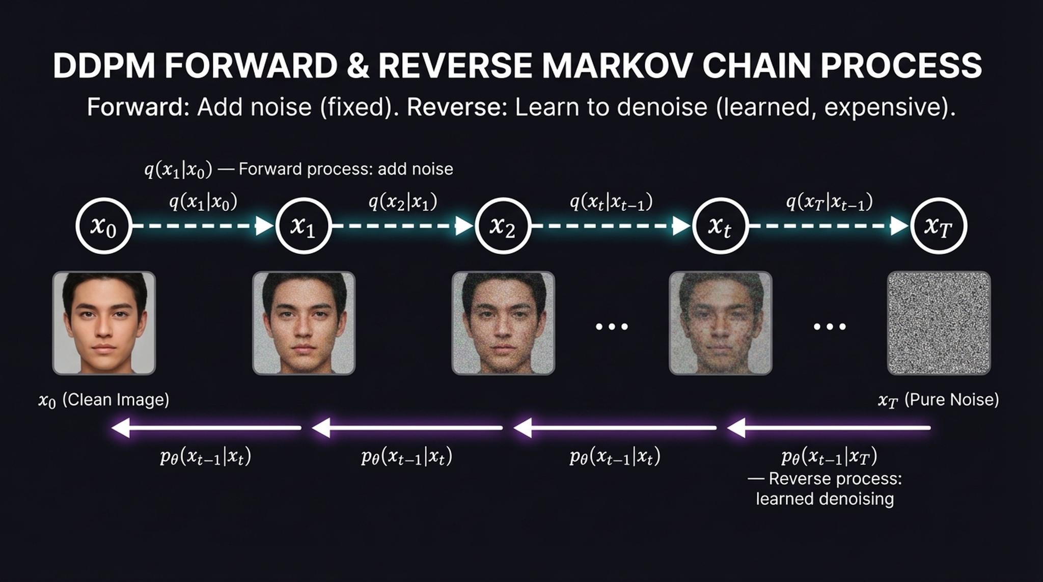
The mathematical core of a diffusion model is two opposing Markov chains. The forward chain is fixed and cheap. The reverse chain is learned and expensive. Understanding this asymmetry is essential.

The forward process \(q\) takes a clean image \(\mathbf{x}_0\) and sequentially injects small amounts of Gaussian noise at each step until, after \(T\) steps (typically 1,000), the signal is completely destroyed and we’re left with pure static \(\mathbf{x}_T \sim \mathbf{N}(0, I)\):

$$q(\mathbf{x}_t | \mathbf{x}_{t-1}) = \mathbf{N}(\mathbf{x}_t; \sqrt{1 – \beta_t}\, \mathbf{x}_{t-1},\; \beta_t \mathbf{I})$$

Think of this as dissolving a sugar cube in water — deterministic in its overall direction toward maximum entropy, even though the exact molecular path is stochastic. No neural network is needed here; it’s pure scheduled noise injection.

The reverse process \(p_\theta\) is where the learning happens. Starting from pure noise \(\mathbf{x}_T\), a neural network learns to undo each corruption step, predicting a slightly cleaner version at each iteration:

$$p_\theta(\mathbf{x}_{t-1} | \mathbf{x}_t) = \mathbf{N}(\mathbf{x}_{t-1};\; \mu_\theta(\mathbf{x}_t, t),\; \sigma_t^2 \mathbf{I})$$

A critical empirical insight: instead of predicting the final clean image \(\mathbf{x}_0\) from a noisy state, it is far more stable to train the network to predict the specific noise tensor \(\varepsilon\) that was added during that step — and then subtract it.

While the mathematics of this Markov chain are elegant, running thousands of sequential neural network passes directly on high-resolution \(3 \times 512 \times 512\) pixel tensors is computationally agonizing. This brings us to the necessity of Latent Diffusion.

---

3. The VAE — A Neural JPEG Compressor

Before we can generate images, we need to solve the curse of dimensionality. A \(512 \times 512\) RGB image is a vector of 786,432 numbers. Running self-attention over this space incurs a catastrophic \(O(N^2)\) cost. The solution: compress first, diffuse later.

The Variational Autoencoder (VAE) acts as a neural JPEG. The encoder applies a lossy compression that shrinks a \(3 \times 512 \times 512\) pixel image down to a \(4 \times 64 \times 64\) latent tensor — discarding imperceptible high-frequency noise while retaining the core semantic structure. This is a 48× compression ratio (786,432 values → 16,384 values).

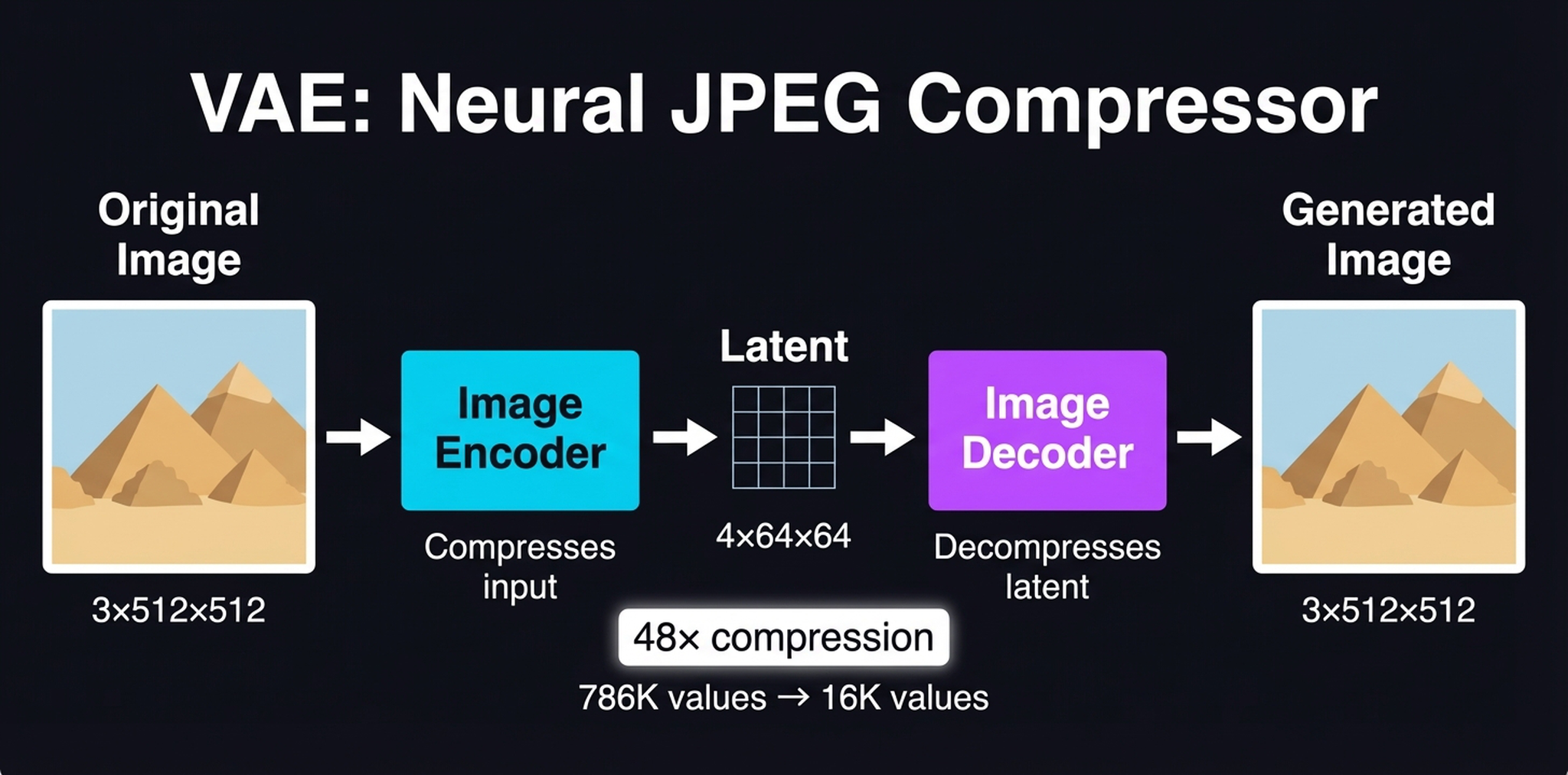
The spatial resolution drops by a factor of 8 (\(512 \div 8 = 64\)) while the channel depth increases from 3 to 4. Once the generative process is complete, the decoder simply decompresses that latent tensor back into a visually faithful \(512 \times 512\) output image. This compression is the key to Stable Diffusion’s efficiency — it makes consumer-GPU inference possible.

---

4. VAE Quality Proof: Original vs. Reconstruction

Before we trust our entire generative pipeline to the latent space, we need to verify that the VAE preserves what actually matters. The test is simple: encode an image into the \(4 \times 64 \times 64\) latent bottleneck, decode it back, and compare.

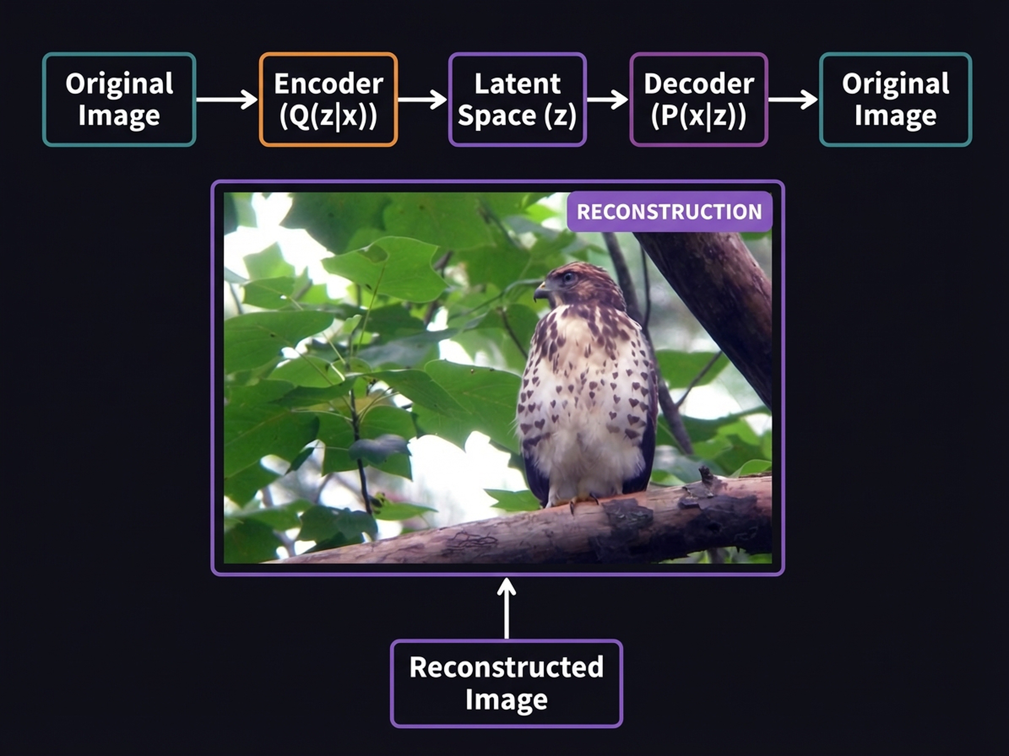
Think of the VAE as a highly optimized neural JPEG: it strategically discards pixel-level high-frequency noise that our visual system barely notices, while perfectly preserving global composition, background bokeh, and semantic identity. The reconstruction isn’t mathematically pixel-perfect — if you subtract the two tensors, the delta won’t be zero — but it shouldn’t be. What matters is that every visual feature carrying meaning survived the 48× compression, proving we can safely perform our computationally expensive diffusion math entirely in the latent space.

---

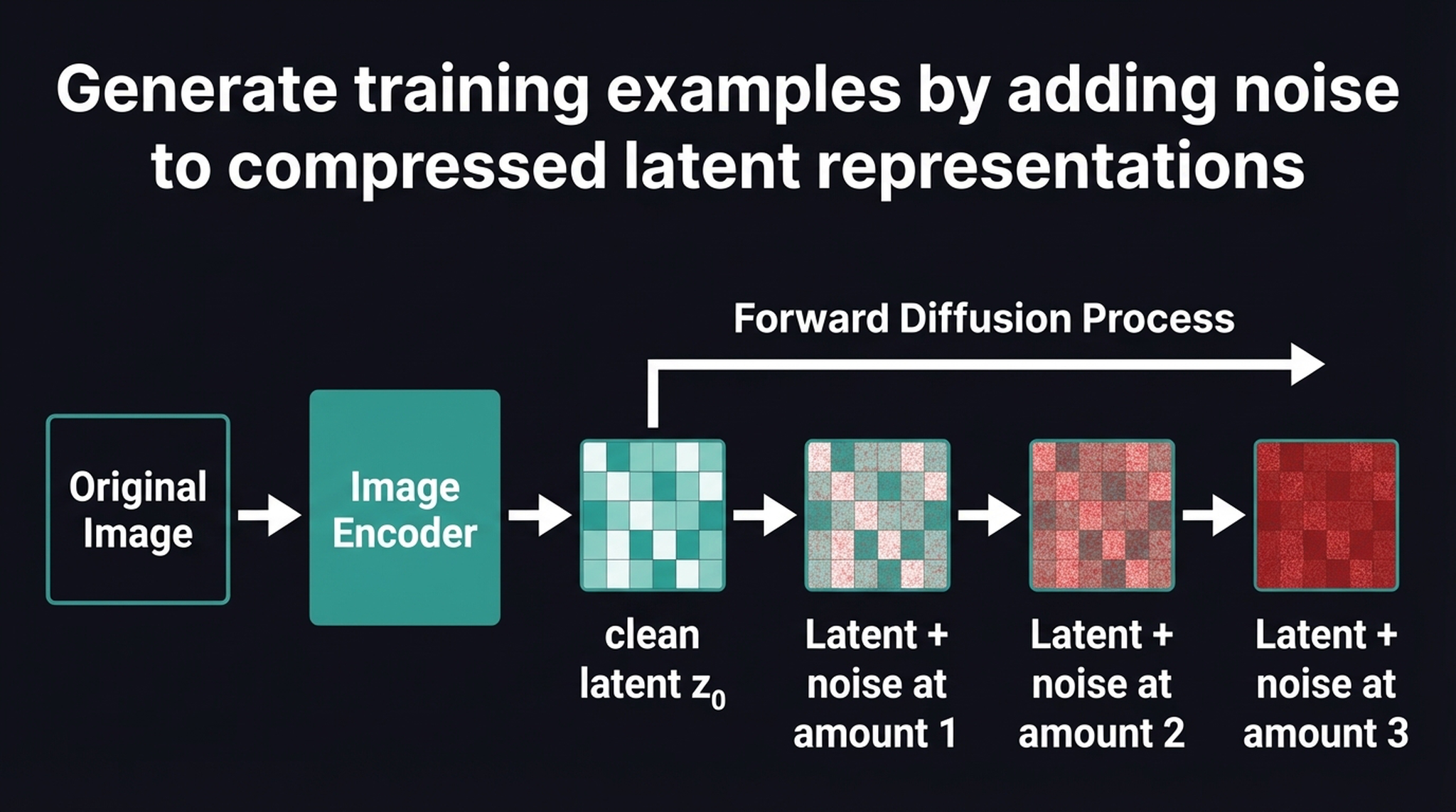
5. Forward Diffusion in Latent Space

Here is where Stable Diffusion fundamentally diverges from standard pixel-space diffusion models. Instead of adding noise directly to a \(3 \times 512 \times 512\) image, we first pass the image through the VAE encoder to extract a compressed \(4 \times 64 \times 64\) latent representation \(z_0\).

The forward diffusion process then injects Gaussian noise exclusively into this latent tensor at various timesteps \(t\). By constructing our training data entirely within this compressed space — mapping a noisy latent \(z_t\) to the specific noise \(\varepsilon\) added at that step — we reduce spatial complexity by 64×, making training vastly cheaper and faster without losing semantic detail.

A critical subtlety: because we have a closed-form expression for the noise schedule, we can compute \(z_t\) at any timestep directly from \(z_0\) without iterating through all previous steps:

$$z_t = \sqrt{\bar{\alpha}_t}\, z_0 + \sqrt{1 – \bar{\alpha}_t}\, \varepsilon, \quad \varepsilon \sim \mathbf{N}(0, I)$$

This is fast, requires no neural network, and allows random sampling of timesteps during training — a key efficiency trick.

---

6. The Complete Forward + Reverse Process

Let’s bring the whole architecture together. The system has two paths — one for training, one for generation — and they are heavily asymmetric:

Forward (training): Original Image → VAE Encoder → clean latent \(z_0\) → add noise (closed-form) → noisy latent \(z_t\). This is fast and trivial.

Reverse (generation): Pure noise \(z_T\) → UNet Step 1 → UNet Step 2 → … → clean latent \(z_0\) → VAE Decoder → Generated Image. This requires ~50 sequential neural network passes.

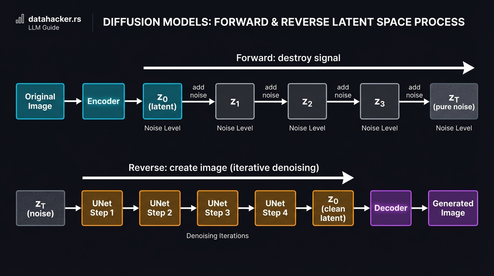
Because this intensive iterative loop happens in the highly compressed latent space rather than high-resolution pixel space, we avoid catastrophic memory limits and can generate novel scenes on a consumer GPU with 8GB VRAM. This spatial compression is the central insight of the Latent Diffusion Model paper (Rombach et al., 2022).

---

7. Single Denoising Step — The Core Subtraction

Every UNet step performs the same fundamental operation. This is the “aha moment” of diffusion models — the mechanism that makes it all work:

1. Take the current noisy latent \(z_t\) and the timestep \(t\)
2. Feed them through the UNet → it outputs a predicted noise pattern \(\hat{\varepsilon}\)
3. Subtract the predicted noise from the noisy image

$$z_{t-1} \approx z_t – \hat{\varepsilon}_\theta(z_t, t, c)$$

(The actual scheduler formula includes scaling factors, but this is the conceptual core.)

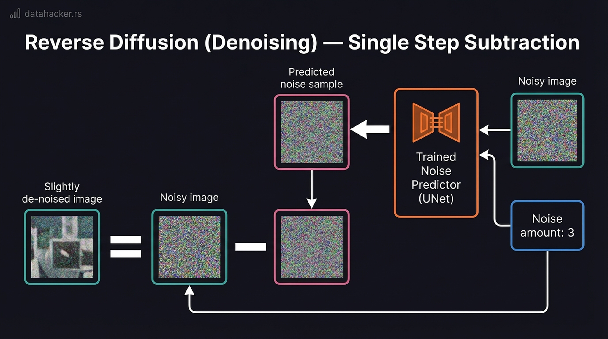
The elegance here is that the network doesn’t need to hallucinate the final image from scratch. It only needs to answer a much simpler question: “given this noisy blob and the current noise level, what does the noise look like?” The image emerges naturally from repeated subtraction.

---

8. Progressive Denoising — Image Emerges from Noise

If we force the VAE decoder to render intermediate latent tensors back into pixel space at various timesteps, we can observe the true mechanics of the reverse process. The result is one of the most satisfying visualizations in machine learning.

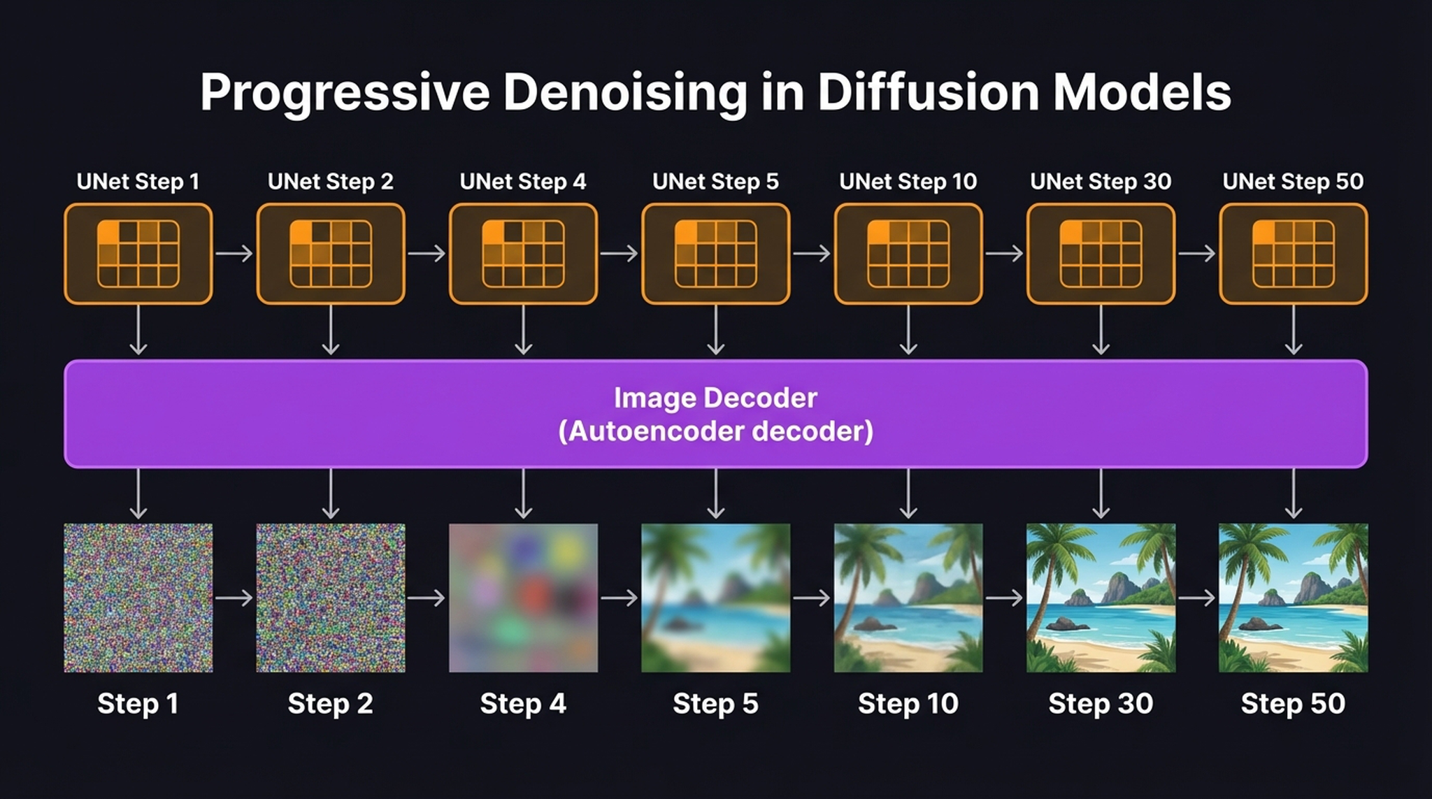
Notice how the denoising schedule behaves like a sculptor. The early UNet passes — operating where the noise variance \(\beta_t\) is highest — hack away massive “chunks” of noise to establish the global composition and color palette. By step 10, the layout of the scene is already locked in. The remaining dozens of steps are dedicated almost entirely to high-frequency refinement — sharpening textures and polishing edges as \(\beta_t\) smoothly anneals toward zero.

Key insight: Diffusion is heavily front-loaded. Global structure is decided in the first ~10% of steps. The remaining 90% is fine-grit sandpaper. This is why accelerated schedulers like DDIM can skip steps with minimal quality loss.

---

9. The Three Components of Stable Diffusion

To deconstruct Stable Diffusion, we must view it not as a monolith, but as an assembly of three distinct, composable modules — each trained separately and typically frozen during inference:

1. Text Encoder (CLIPText) — maps a raw string of text into a dense semantic embedding. It understands the prompt.
2. Image Information Creator (UNet + Scheduler) — the core engine that does the heavy lifting: iteratively sculpting the image structure by removing noise, entirely within latent space.
3. Image Decoder (VAE decoder) — projects the final latent tensor back into pixel space. It decompresses the result.

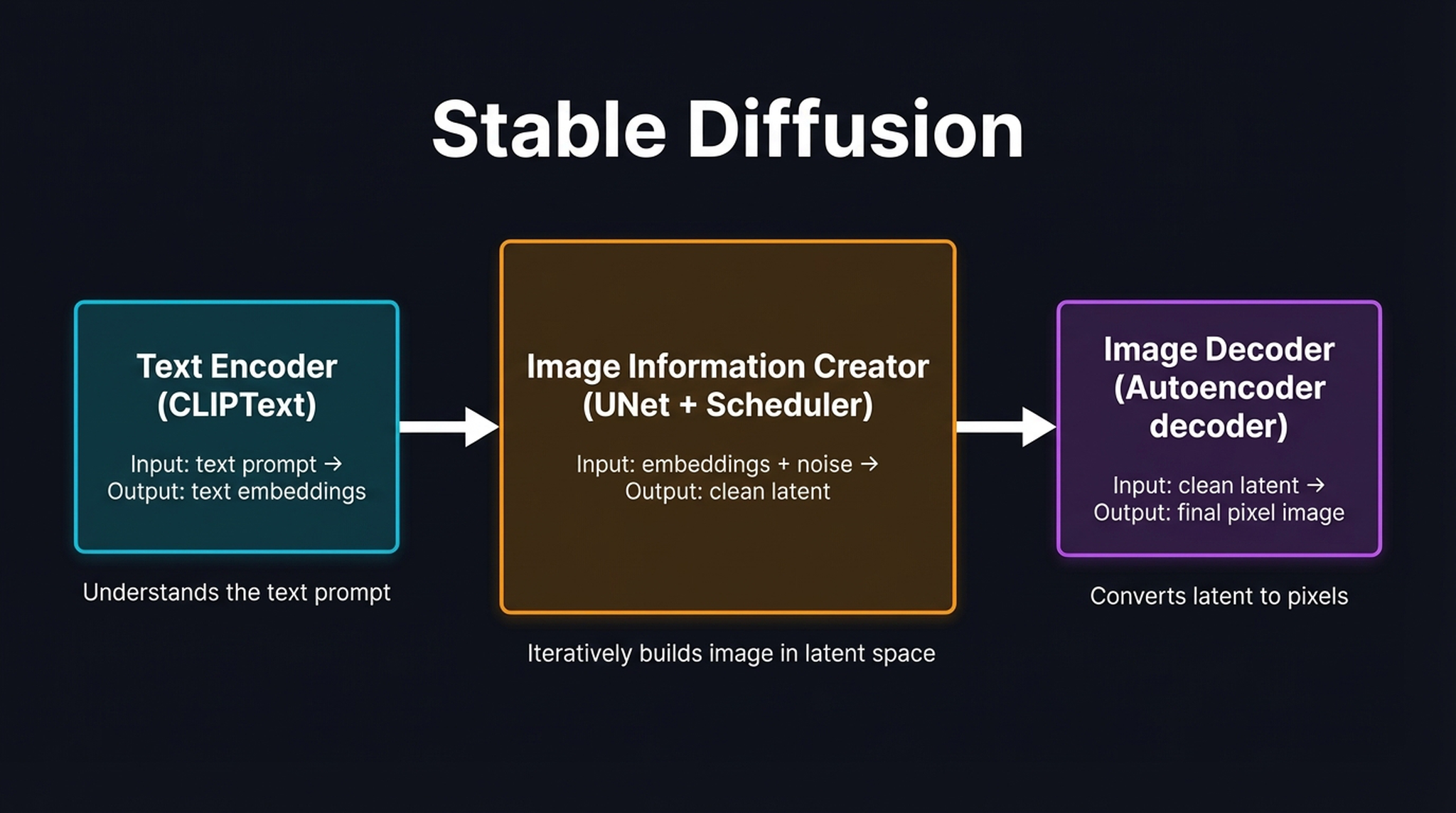
Think of this as a translating assembly line. The Text Encoder acts as the translator, the UNet is the factory floor, and the Image Decoder is the packaging department. Each module has a well-defined input and output; they communicate through precisely shaped tensors.

---

10. The Pipeline with Tensor Dimensions

To appreciate why Stable Diffusion can run on consumer hardware, you have to look closely at the tensor dimensions flowing through the architecture:

• Input text → tokenized to 77 tokens → Text Encoder (CLIPText) → \([77 \times 768]\) token embeddings
• UNet + Scheduler operates on \([4 \times 64 \times 64]\) latent tensors — 48× smaller than pixel space
• Image Decoder outputs the final \([3 \times 512 \times 512]\) RGB image

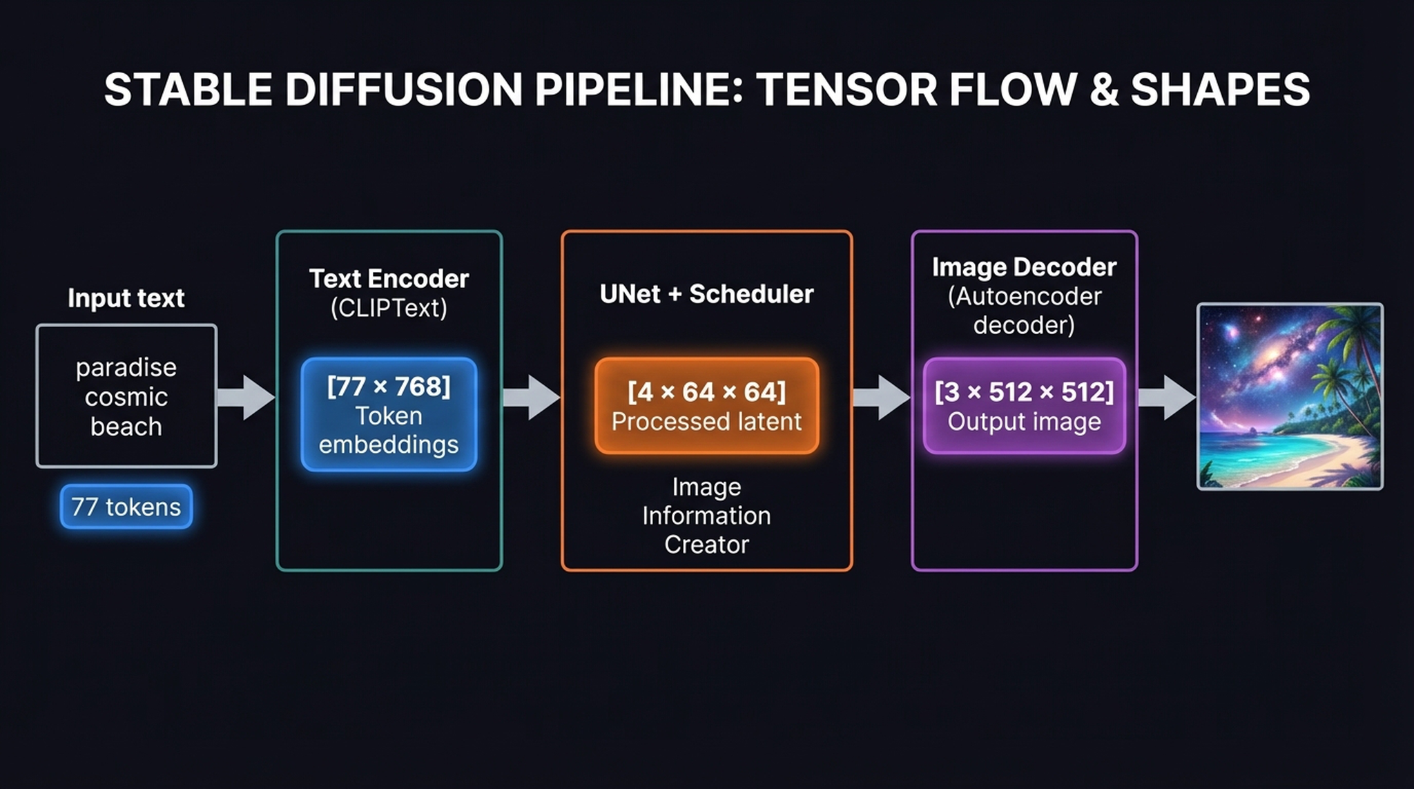
A crucial detail: CLIP retains the full unpooled \(77 \times 768\) token sequence rather than collapsing it into a single summary vector. This is critical — it allows the UNet’s cross-attention mechanisms to dynamically map specific textual concepts (like the word “cosmic”) directly to localized spatial regions (the sky area) as the latent image takes shape.

---

11. CLIP Training: Three Steps to a Shared Embedding Space

To bridge the gap between pixels and language, Stable Diffusion relies on CLIP (Contrastive Language-Image Pre-training) as its translation layer. CLIP was trained on roughly 400 million image-text pairs scraped from the internet, using a three-step contrastive learning loop:

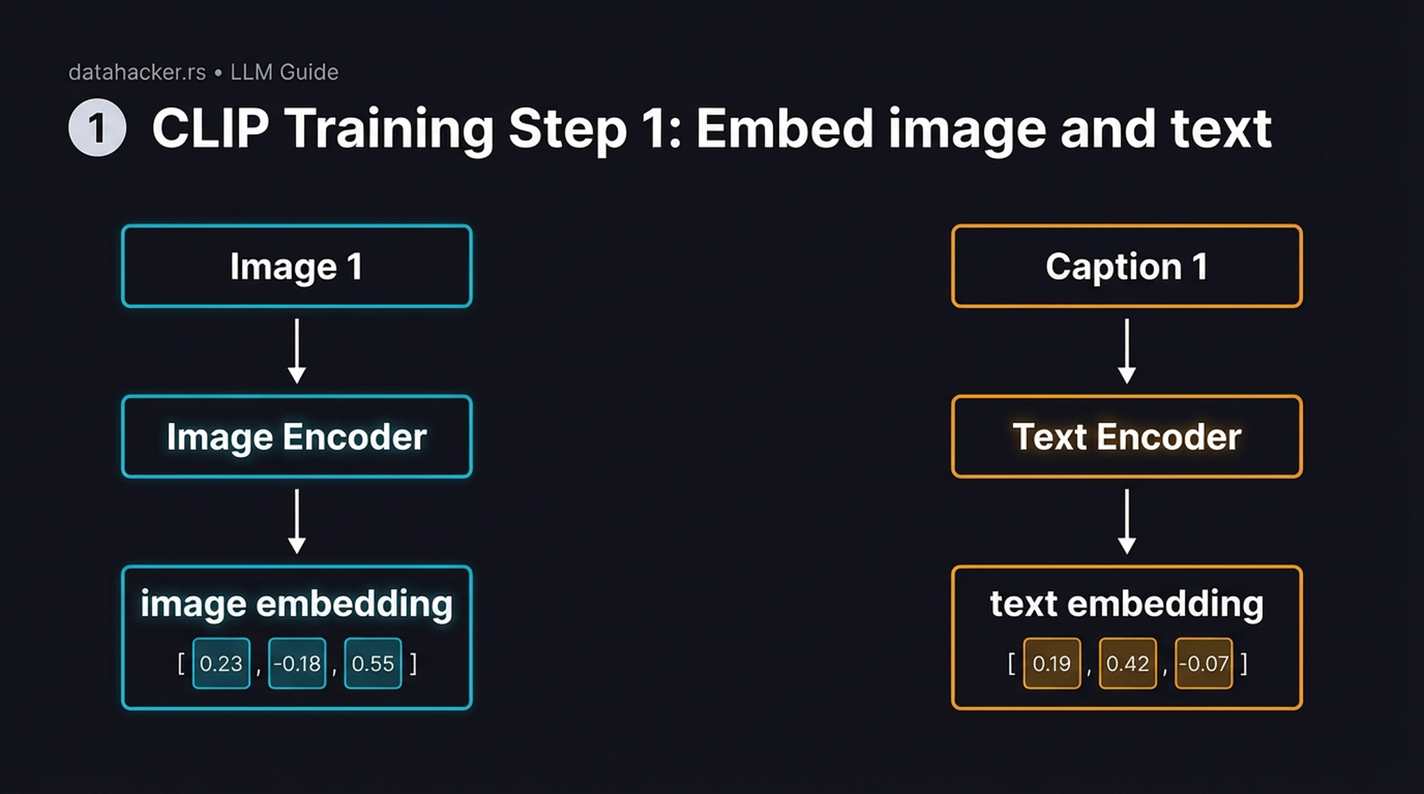
Step 1: Embed — A Vision Transformer encodes the image into a fixed-length vector. Independently, a text Transformer encodes the caption into a vector of the same dimension. At this stage, the two encoders know nothing about each other.

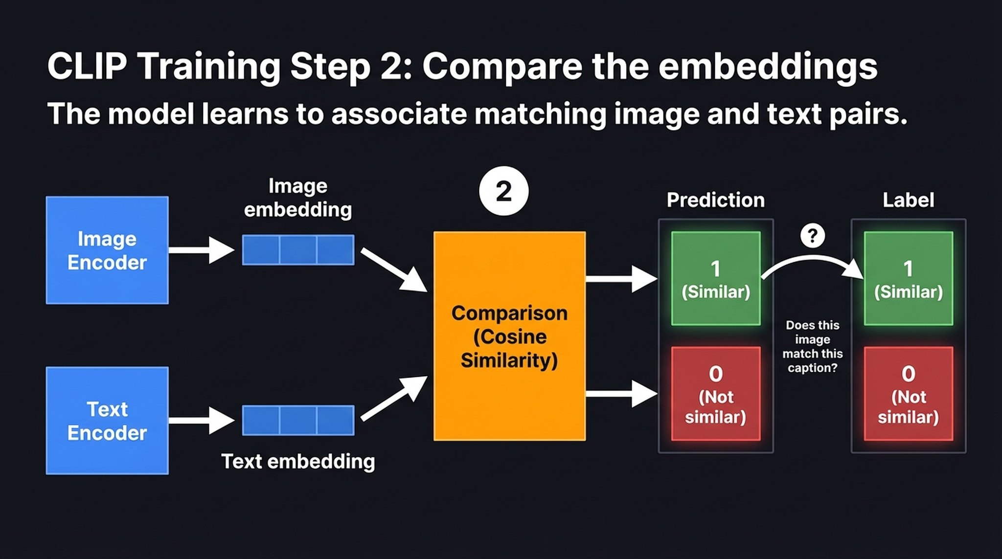
Step 2: Compare — We compute cosine similarity between every image embedding and every text embedding in the batch, forming an \(N \times N\) matrix. Matching pairs (the diagonal) should score high; mismatched pairs should score low.

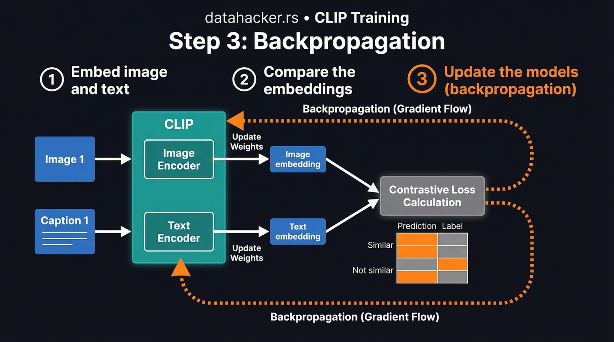
Step 3: Backpropagate — Gradients flow backward from the contrastive loss into both encoders simultaneously, geometrically aligning the shared embedding space. Matched pairs are pulled closer; mismatched pairs are pushed apart.

Because this contrastive training forces the text encoder to deeply understand visual concepts, we can safely discard the image encoder, freeze the text encoder, and use its rich \(77 \times 768\) embeddings to condition our diffusion model. The text encoder becomes the semantic steering wheel for image generation.

---

12. UNet: Three Inputs, One Output

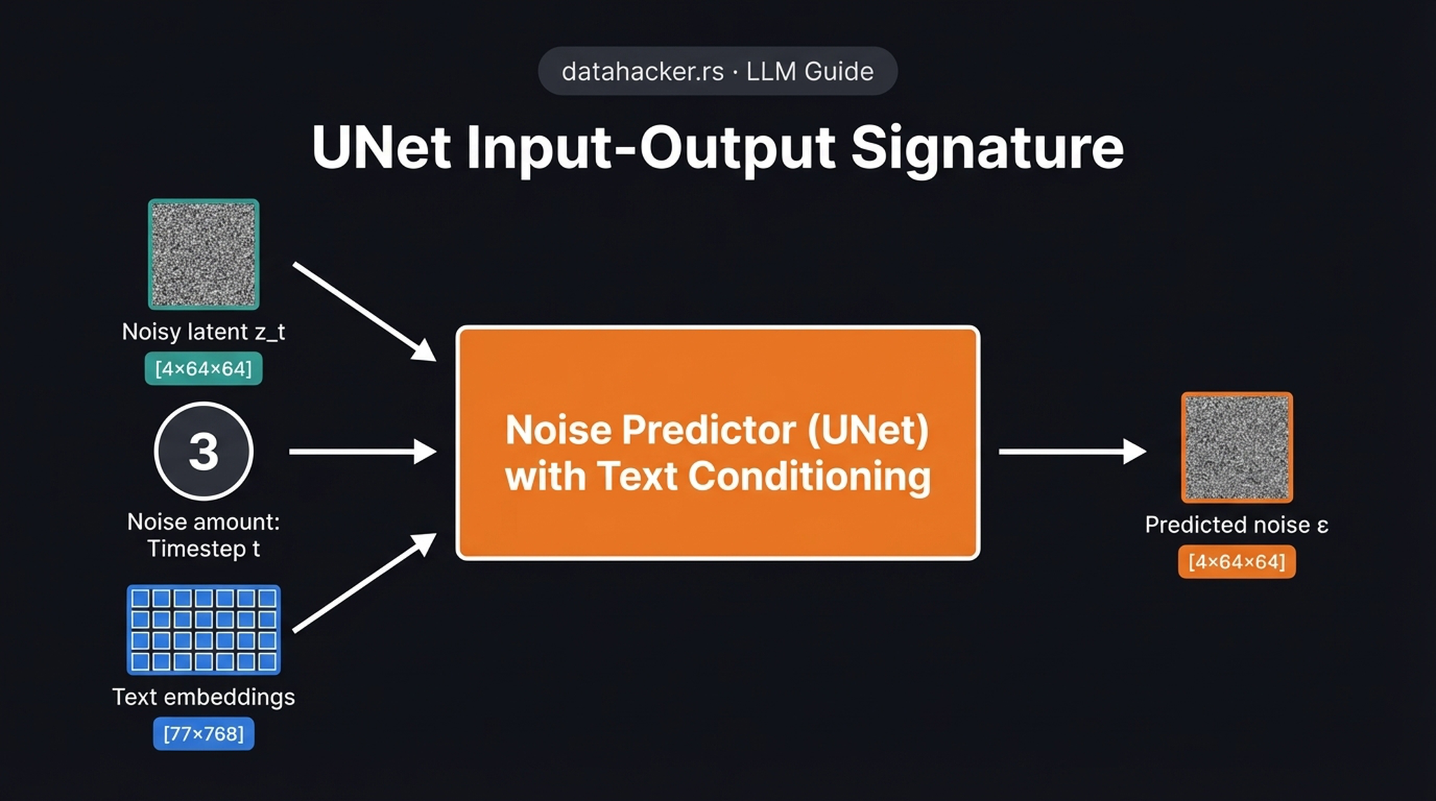
Here we see the complete input-output signature of the conditional UNet \(\varepsilon_\theta\). It takes three distinct inputs:

1. Noisy latent \(z_t\) — a \([4 \times 64 \times 64]\) spatial tensor representing the current state of the image
2. Timestep \(t\) — encoded using sinusoidal positional embeddings (like a Transformer) so the network knows the current noise scale
3. Text embeddings — a \([77 \times 768]\) tensor of token embeddings from the frozen CLIP text encoder

And produces one output: the predicted noise \(\hat{\varepsilon}\) — a \([4 \times 64 \times 64]\) tensor of the exact same shape as the input latent.

The network explicitly needs the timestep because a heavily noised input requires entirely different feature extraction logic than a nearly clean input near the end of the chain. The training objective is surprisingly simple:

$$\mathbf{L} = \| \varepsilon – \varepsilon_\theta(z_t, t, c) \|^2$$

Minimize the squared difference between the actual noise added and the network’s prediction. That’s it — a straightforward MSE loss.

---

13. Inside the UNet — ResNet + Cross-Attention

To understand how text mathematically guides image generation, we must look inside the UNet’s alternating layers. The architecture repeats two types of blocks:

• ResNet blocks (spatial processing) — these process the latent’s spatial features and absorb the timestep embedding via FiLM-style conditioning (Feature-wise Linear Modulation). Think of them as the sculptor’s hands — they shape the material based on how much noise remains.
• Cross-Attention blocks (text conditioning) — these are where the text embeddings physically intersect with the spatial features. The spatial features become the Query (Q), while the text embeddings provide the Keys (K) and Values (V):

$$\text{Attention}(Q, K, V) = \text{softmax}\left(\frac{QK^T}{\sqrt{d}}\right) V$$

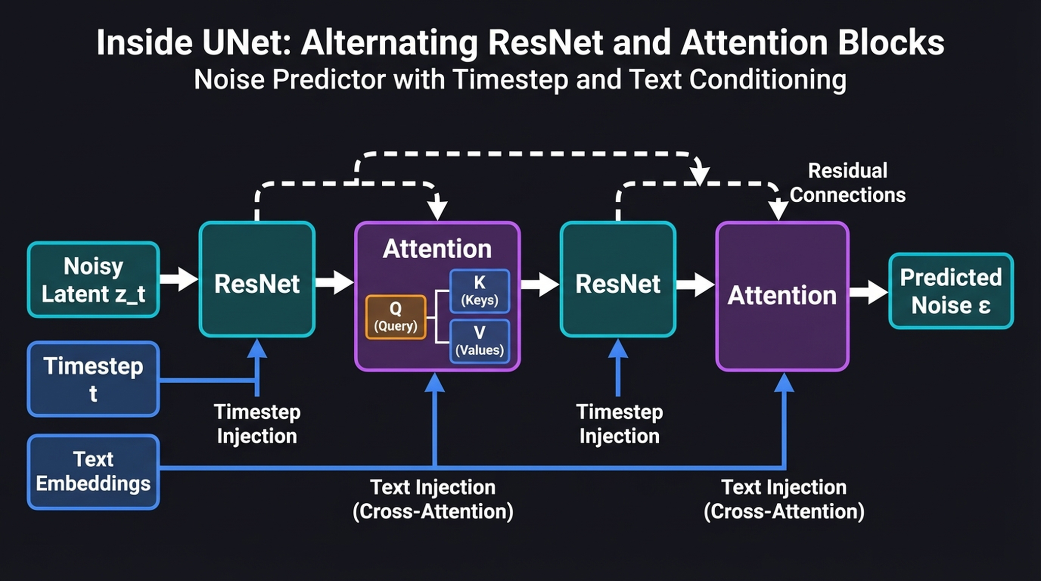
This cross-attention mechanism acts as a GPS: it allows specific regions of the image to “look up” matching semantic concepts from specific text tokens. When generating a “cosmic beach,” the sky region’s Query vectors will attend strongly to the “cosmic” token’s Key/Value, while the foreground attends to “beach.” The text doesn’t control the image globally — it guides it locally through attention weights.

---

14. The UNet Training Loop

The training loop is elegantly simple — four steps, repeated millions of times:

1. Pick a training example — take a real image, encode it via the VAE, sample a random timestep \(t\), and add the corresponding amount of noise to get \(z_t\)
2. Predict noise — feed \(z_t\), \(t\), and the text embeddings through the UNet → get predicted noise \(\hat{\varepsilon}\)
3. Compare to actual noise — compute \(\text{MSE}(\varepsilon, \hat{\varepsilon})\)
4. Update model — backpropagate and adjust UNet weights

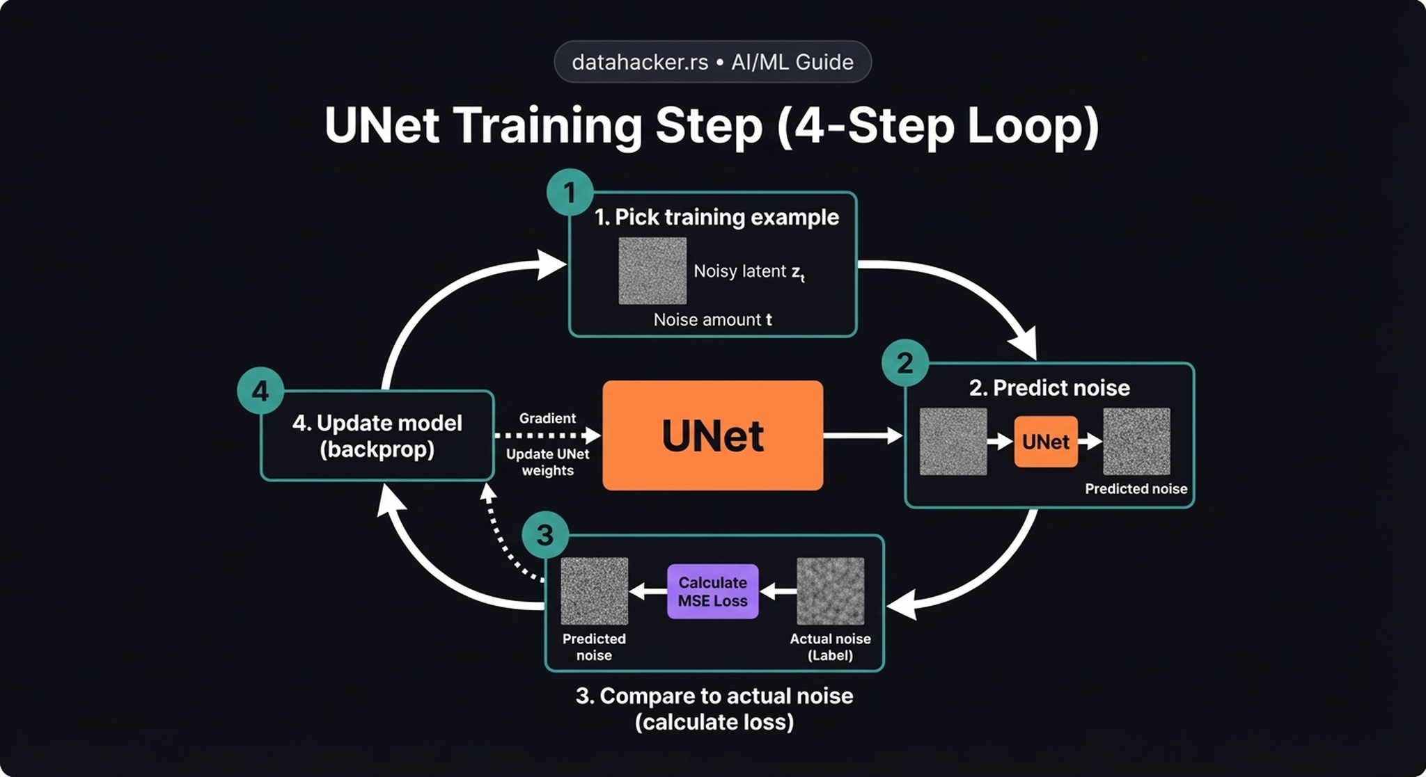
Key insight: This is self-supervised learning. We added the noise ourselves, so we always have perfect labels. No human annotation is needed. A finite set of images effectively becomes an infinite dataset — each image can be corrupted at any of 1,000 timesteps with any random noise sample.

---

15. Training Dataset Structure

Let’s look at how a training batch is actually constructed. Each row is one training example with:

• Input: a random timestep \(t\) + the noisy latent \(z_t\) + the text embeddings from the caption
• Target/Label: the exact noise tensor \(\varepsilon\) that was added

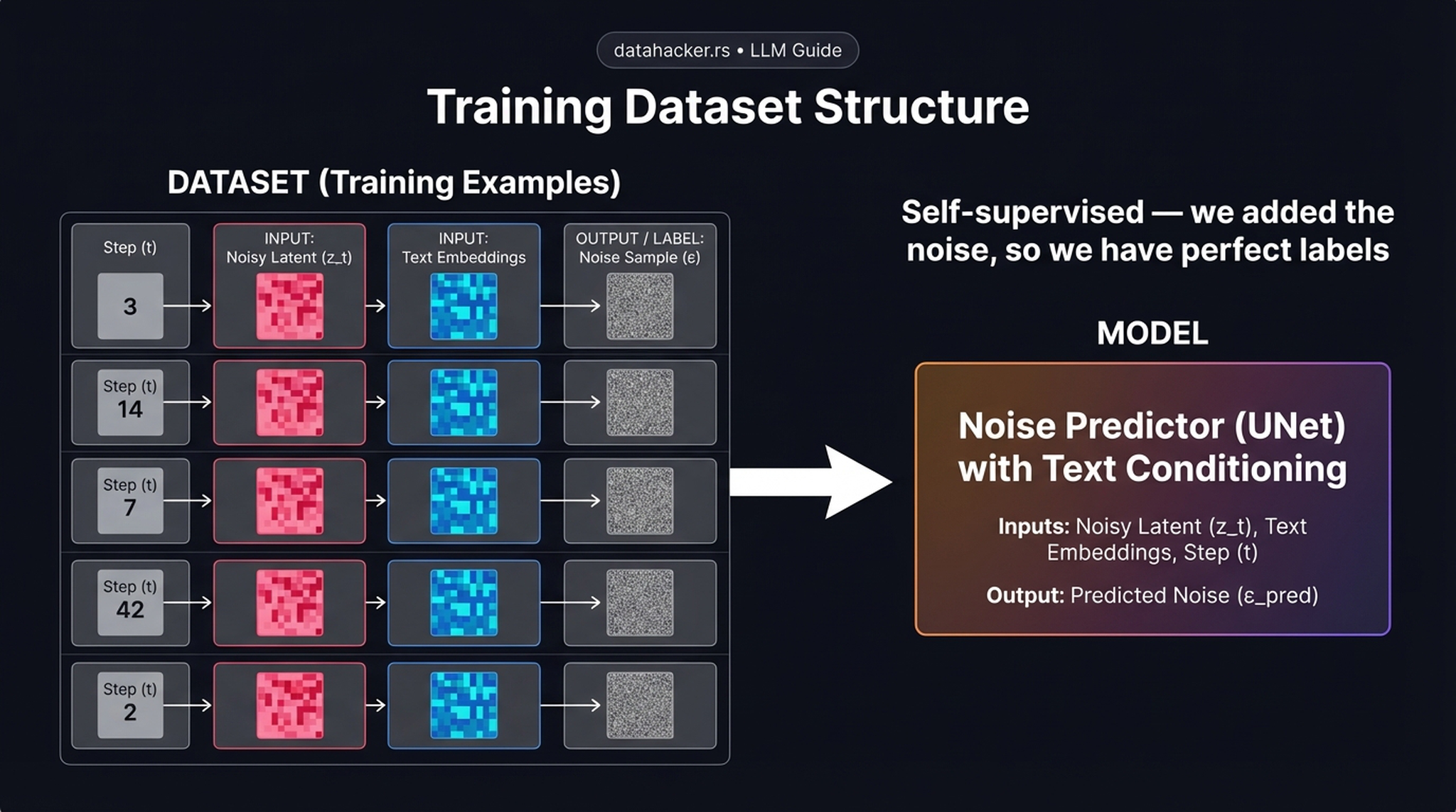
By randomly sampling \(t\) and \(\varepsilon\) dynamically during training, a finite set of images effectively becomes an infinite dataset of unique noisy training pairs. This is what makes diffusion models scale so elegantly without requiring massive human-annotated datasets — the generation problem becomes a robust, self-supervised regression task.

---

16. Conditional Generation on MNIST

Before tackling the complexity of \(3 \times 512 \times 512\) text-to-image generation, it is instructive to validate conditional diffusion on a simpler \(1 \times 28 \times 28\) problem like MNIST.

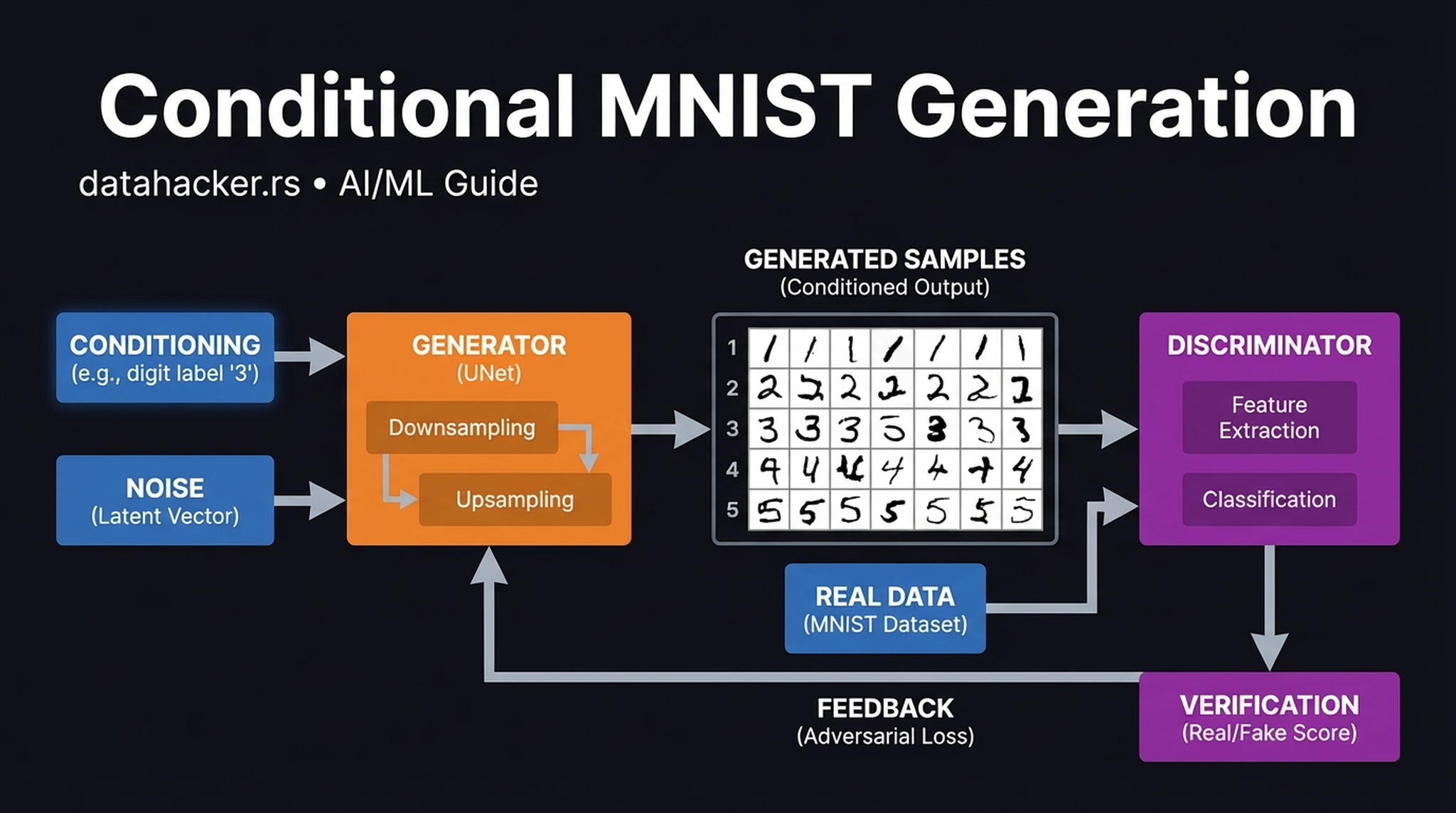
The class embedding successfully biases the reverse diffusion trajectory, steering the denoising process down five completely distinct paths without bleeding into adjacent classes. Think of the conditioning label as a GPS destination — the model finds multiple valid, distinct routes from various noisy starting points to that destination.

---

17. Classifier-Free Guidance

Conditioning is not binary — it’s a continuous dial. The Classifier-Free Guidance (CFG) scale \(w\) controls how strictly the model follows the conditioning signal:

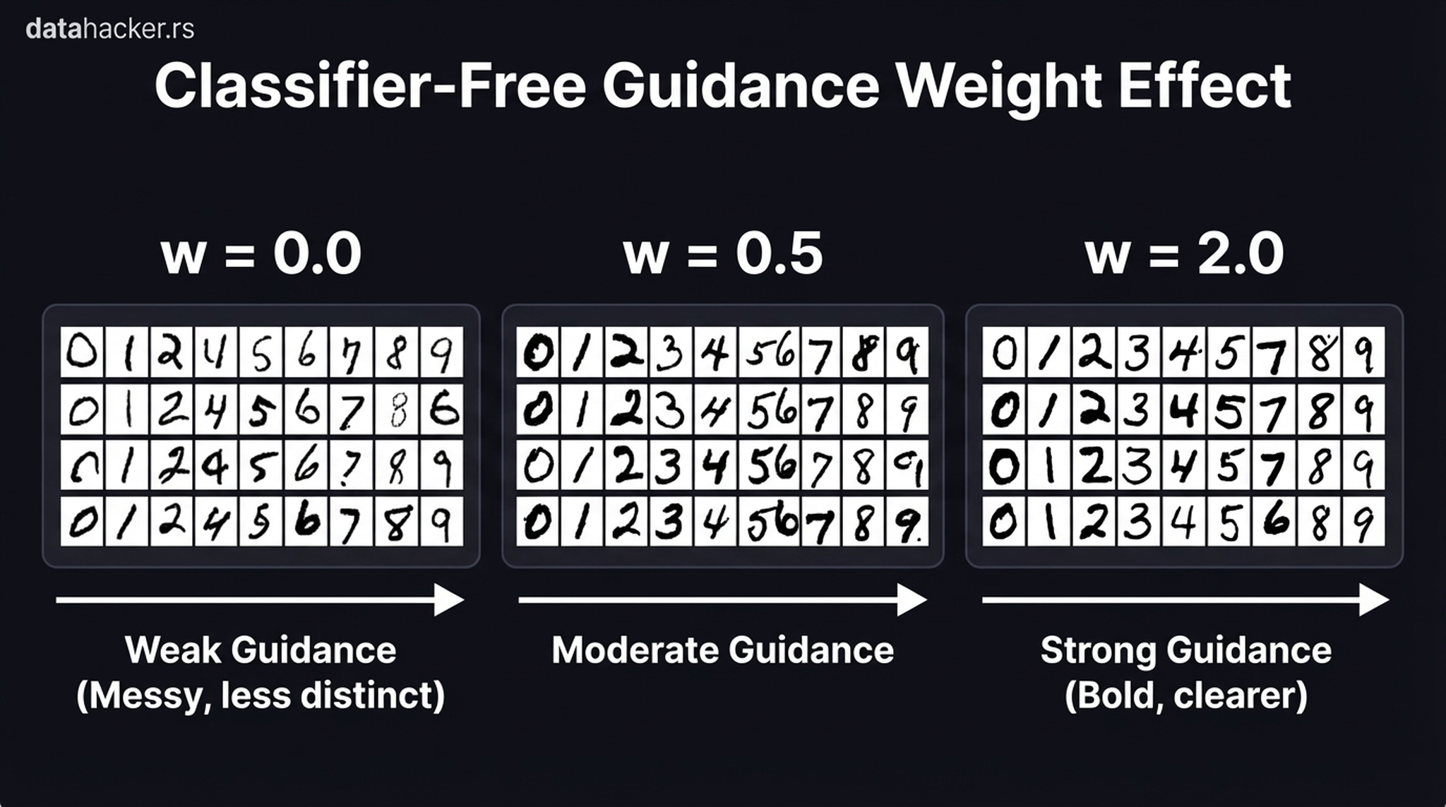
At \(w = 0\), the model is effectively ignoring the conditioning signal — high diversity but poor fidelity (wrong classes appear). At \(w = 2.0\), the model becomes extremely strict: every digit is bold and unmistakable, but stylistic diversity collapses. In practice, Stable Diffusion uses \(w \approx 7.5\) — a carefully chosen balance between prompt adherence and creative freedom.

Mathematically, CFG works by running the UNet twice per step — once with the conditioning and once without — then extrapolating in the direction of the conditioned output:

$$\hat{\varepsilon} = \varepsilon_\text{uncond} + w \cdot (\varepsilon_\text{cond} – \varepsilon_\text{uncond})$$

This doubles the compute per step but dramatically improves output quality. It’s why Stable Diffusion inference is slower than you might expect from the step count alone.

---

18. LDM Complete Architecture

This is the diagram you come back to. Everything we’ve built — the VAE, the diffusion process, the CLIP encoder, the cross-attention conditioning — lives inside this one figure.

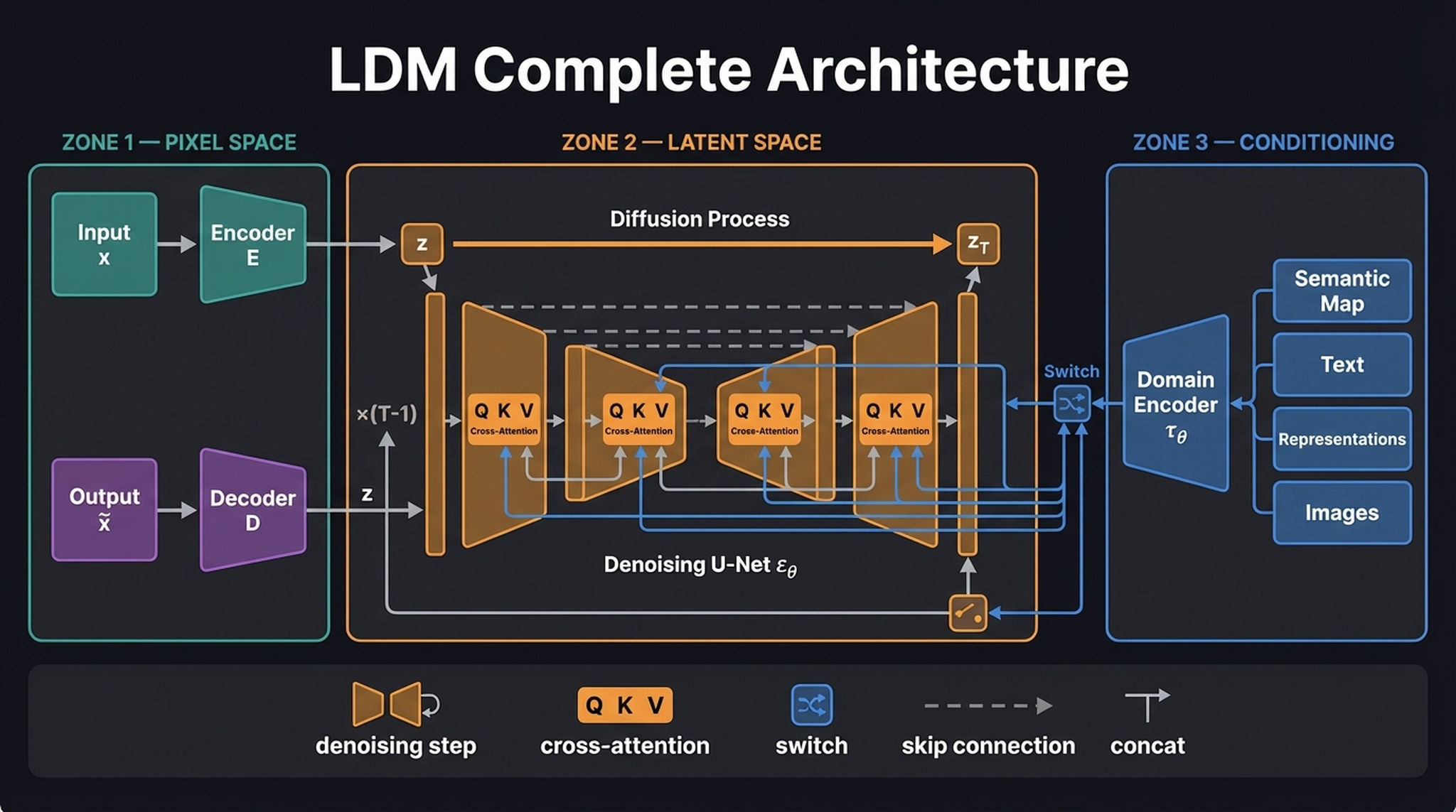
Reading left to right:

• Pixel Space (left): Our VAE acts as a neural JPEG, compressing \(x\) into latent \(z\) via encoder \(\mathbf{E}\). The decoder \(\mathbf{D}\) reconstructs \(z\) back to pixel space as \(\tilde{x}\).
• Latent Space (center): The forward diffusion process corrupts \(z\) into \(z_T\). The Denoising U-Net \(\varepsilon_\theta\) iteratively recovers it through \(T{-}1\) reverse steps. Inside the UNet, QKV cross-attention blocks connect the spatial features to external conditioning.
• Conditioning (right): Text, semantic maps, or any other modality is processed by a domain-specific encoder \(\tau_\theta\). The outputs feed the U-Net’s cross-attention as Keys (K) and Values (V), while the spatial features provide Queries (Q).

The “switch” icon at the junction indicates that conditioning can either enter via cross-attention (multiplicative, attention-weighted) or via direct concatenation with the latent tensor. Text conditioning uses cross-attention; spatial conditioning (like segmentation maps) typically uses concatenation.

---

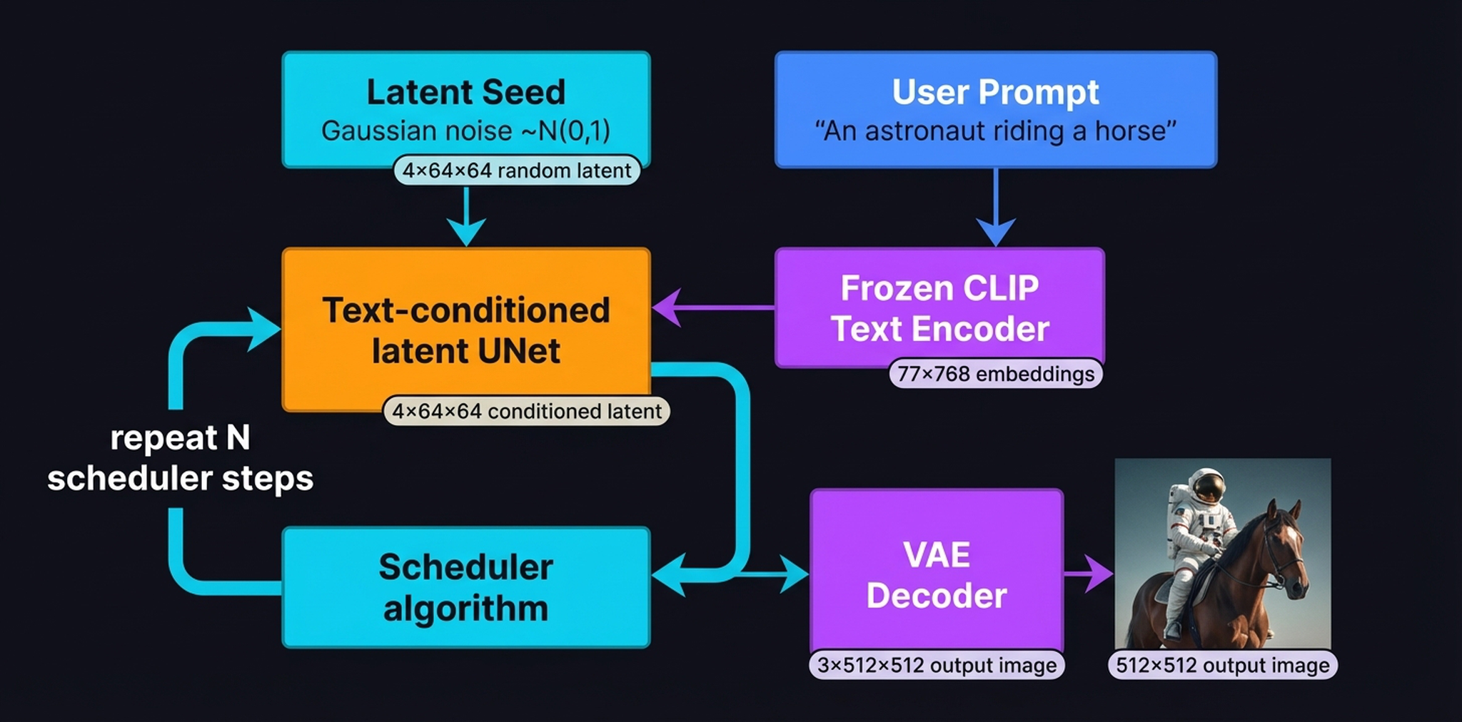
19. The Full Inference Pipeline

Now let’s trace a single inference run from start to finish. Two inputs enter the system:

1. Latent Seed: a \(4 \times 64 \times 64\) tensor of Gaussian noise \(z_T \sim \mathbf{N}(0, I)\)
2. User Prompt: “An astronaut riding a horse” → Frozen CLIP Text Encoder → \([77 \times 768]\) embeddings

The UNet + Scheduler loop is where all the computation happens. Over \(N\) scheduler iterations (typically 50 steps with DDIM, which mathematically approximates the trajectory to skip steps), the UNet progressively predicts and removes noise. The \(77 \times 768\) CLIP text embeddings remain completely frozen throughout — a static conditioning anchor that guides the UNet at every single iteration.

Only at the very end does the VAE Decoder transform the clean \(4 \times 64 \times 64\) latent tensor \(z_0\) into a \(3 \times 512 \times 512\) RGB image. This final decode happens once, not at every step — another key efficiency gain of latent diffusion.

---

20. LDM Architecture — QKV Cross-Attention Focus

Our final diagram provides an alternative perspective on the LDM architecture, zooming into the cross-attention plumbing that makes flexible conditioning possible.

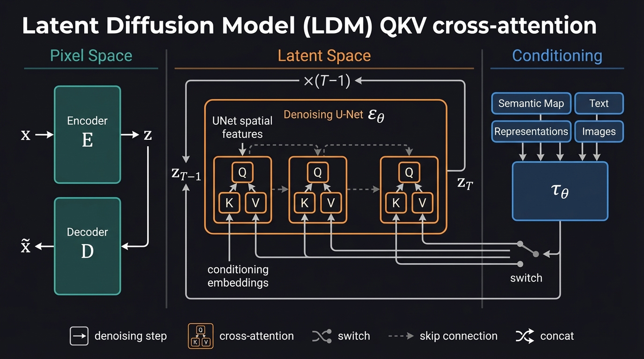
The key insight of this view: the conditioning encoder \(\tau_\theta\) is brilliantly flexible. Whether you feed it text via CLIP to get a \(77 \times 768\) tensor, or a segmentation map via a CNN, or even another image via a vision encoder — as long as \(\tau_\theta\) formats the output into a sequence of vectors, the UNet’s cross-attention layers can query it without changing their underlying architecture. This modular design is why Stable Diffusion has been so successfully extended to ControlNet, IP-Adapter, and dozens of other conditioning mechanisms.

The entire framework boils down to two ideas, unified in one pipeline. The VAE compresses the problem into a space where diffusion is computationally tractable, crunching \(3 \times 512 \times 512\) images into \(4 \times 64 \times 64\) latents. CLIP and cross-attention give that denoising process a semantic compass. Together, they are Stable Diffusion.

---

21. Summary

Let’s crystallize what we’ve built in this post:

Component	Role	Key Tensor
VAE Encoder \(\mathbf{E}\)	Compress pixels → latent	\(3 \times 512 \times 512 \to 4 \times 64 \times 64\)
VAE Decoder \(\mathbf{D}\)	Decompress latent → pixels	\(4 \times 64 \times 64 \to 3 \times 512 \times 512\)
CLIP Text Encoder	Translate prompt → embeddings	\(\text{string} \to [77 \times 768]\)
UNet \(\varepsilon_\theta\)	Predict noise (conditioned)	\([4 \times 64 \times 64] \to [4 \times 64 \times 64]\)
Scheduler	Control denoising trajectory	Timesteps + scaling factors

The generation process:

1. Sample Gaussian noise \(z_T \sim \mathbf{N}(0, I)\) as a \(4 \times 64 \times 64\) tensor
2. Encode the text prompt via frozen CLIP → \([77 \times 768]\) embeddings
3. For each scheduler step \(t = T, T{-}1, \ldots, 1\): feed \(z_t\), \(t\), and text embeddings into the UNet → predict \(\hat{\varepsilon}\) → subtract to get \(z_{t-1}\)
4. Decode the final clean latent \(z_0\) via the VAE Decoder → \(3 \times 512 \times 512\) image

That’s it. Every piece fits. The VAE makes the problem tractable. CLIP makes it steerable. Cross-attention makes it precise. And the iterative denoising makes it beautiful.

In the next post, we’ll open the PyTorch source code and trace these tensors through actual function calls.

Take care! 🙂