#002 GANs – Supervised vs. Unsupervised Learning and Discriminative vs. Generative

Highlights: GANs and classical Deep Learning methods (classification, object detection) are similar, but they are also fundamentally different in nature. Reviewing their properties will be the topic of this post. Therefore, before we proceed further with the GANs series, it will be useful to refresh and recap what is supervised and unsupervised learning. In addition, we will explain the difference between discriminative and generative models. Finally, we will introduce latent variables, since they are an important concept in GANs.
Tutorial Overview:
1. Supervised vs. Unsupervised learning
The most common task in Computer Vision and Machine Learning is classification[1]. For instance, we have a set of data samples and those samples are labelled according to what class they belong to. Our goal is to learn a function that maps the data to the classes. For instance, we have used supervised classifications in many posts in our PyTorch series. For instance, within the post Logistic Regression in PyTorch, we have explored Binary Classification as one basic supervised learning problem.

Moreover, the data samples can be images \(x \) of cats and non-cats. Basically, for any given image we want to know whether it is a cat or not (vector \(y \)). Therefore, our goal in supervised learning is to learn a function that will map an input image into a \(\left\{ 0,1\right\} class \).
Naturally, the number of classes can be larger than two. For instance, a well-known MNIST dataset consists of images of handwritten digit numbers. In this case, we have to design a function that will map an input image of any given digit into a class from 0 to 9.
The other class of problems you are probably familiar with is unsupervised learning. Now, in contrast, we do not have any labels along with our dataset. Nowadays, in the era of super large datasets, the problem of data labelling is becoming more obvious. Due to such a large quantity of data, researchers usually refer to those datasets as “datasets in the wild”. Therefore, our task is more challenging than in a supervised learning framework and our goal is to understand the hidden and/or underlying structure that exists in data. In this way, we can gain insights into the explanatory factors that are hidden in our datasets.
One well-known example of unsupervised learning is clustering. For instance, you can apply a kMeans algorithm on an MNIST dataset of handwritten digits. If we choose \(k=10 \), we will obtain interesting clusters where the same digits will mainly cluster in one class (group). Naturally, in the more complex dataset, the parameter value \(k \) we do not know in advance, and therefore, the problem becomes more challenging.
2. Discriminative vs. Generative
Now comes the most important part of the post. The difference between machine learning models can be depicted in the following graph:
In standard problems that we are solving, we usually have an input image \(y \) and a label \(y \). Label \(y \) can be known to us and in this case we are tackling supervised learning problems. On the other hand, the label \(y \) can be unknown and in that case we have an unsupervised learning problem.
If we cast our problem onto the probabilistic perspective, we will have the following:
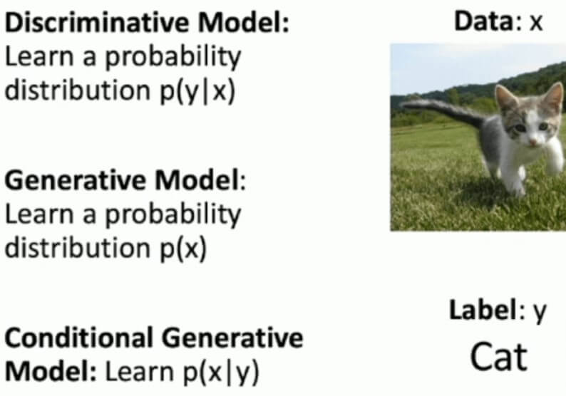
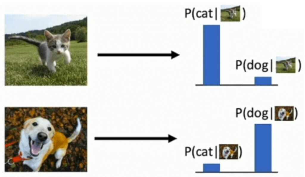
- DISCRIMINATIVE MODEL. The goal is to learn a probability function \(p(y|x) \). In simple words, we need to learn a function that is going to tell us what is the probability that for a given image \(x \), we have a label \(y \). An example is a cat image, as shown in the image above, and our goal is to develop a model that will output a probability value that there is indeed a cat in the image.
- GENERATIVE MODEL. In this case the goal of the model is to “simply” learn a probability function \(p(x) \). In this case, we do not know the class of the image. Hence, for a given image we have to determine for a given image what the probability of occurrence is. For instance, we can assume that we are dealing with all images that are posted on Instagram. If we see, an image of a cat or a selfie, well, the probability for such images is rather high. On the other hand, seeing images of mathematical equations is possible, but much less likely :-).
Let’s review these topics more closely. The following graphs represent the difference between Discriminative and Generative models in the best possible way. You have probably used the LDA (Linear Discriminant Analysis) algorithm for classification tasks. For a given input data, the model needs to learn how to bring a classification decision.
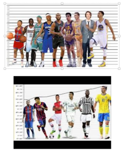
Commonly, in data analysis, we have data that follow a certain distribution. Some variables may, for instance, follow a Gaussian distribution. For example, the height of basketball players can be described as a Gaussian distribution. Many algorithms in machine learning are developed to estimate the parameters of an unknown probability distribution. For instance, there is a well-known Gaussian Mixture Model – GMM.
Another task of interest is the idea of sample generation. In this context, we’re given input samples and we want to develop a model that generates brand-new samples which represent those inputs.
This is the idea with the generation of fake faces that we have shown in the previous post. The core question behind generative modelling is how we can learn and model a probability distribution of some data. Then, how we can apply this distribution to generate new data that is very similar to the original dataset, and yet different enough so that we can consider the data as a novel.
In machine learning, we have already encountered some problems with probability estimates. Hmmm…Bayes! Naïve Bayes. And there was also the Gaussian Mixture Model method. In case you need a refresher, we refer to an excellent book of Jake VanderPlas Data Science Handbook. There, you can find an example of GMM and the generation of MNIST dataset.
Outliers
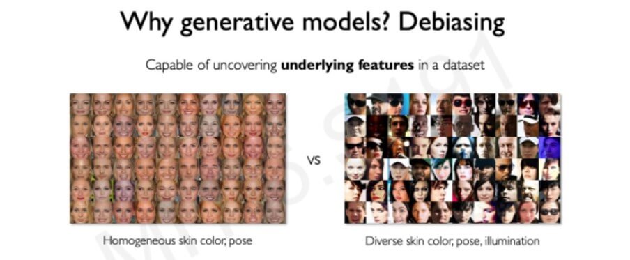
Another great example is the detection of outliers. For instance, the detection of outliers in a dataset for self-driving cars is very important. In general, you want to train the model on conditions that are very common. That can be for instance a sunny day. But you also want the networks to be trained during conditions that are rare. For this application, the data augmentation and generation methods can be very important!
This can be illustrated in the following image where weather conditions are illustrated according to their probabilities. For instance, we can imagine that the very unlikely road condition occurrences are located in the tail of the distribution. You may ask what kind of distribution is that and how do you generate it. For now, we can just assume that a latent variable for “common weather” is discovered in a dataset. Hence, common weather may be a sunny and rainy day, whereas a storm blizzard can be regarded as an unlikely event. In case some things are unclear so far, don’t worry! We will talk a lot about this later on.
Therefore, generative models can be used to actually detect the outliers that exist within a training dataset. Moreover, similar “outliers” can be further generated in a realistic fashion and later used to train a more robust model.
3. Latent Variables
Latent variables are usually not measured directly within a dataset. Nevertheless, we say that latent variables capture important interplay among the data features. Moreover, they represent the governing mechanism of how our data examples look like. With the idea of the cocktail party problem, a latent variable can be a source (or original signal) that we are interested in.
However, the only signal that we can record is a mixture of many sound sources. In addition, most of the time we really care only about the underlying generated sources.
For instance, let’s take a look at the example of FastICA that works on synthesized toy signals.
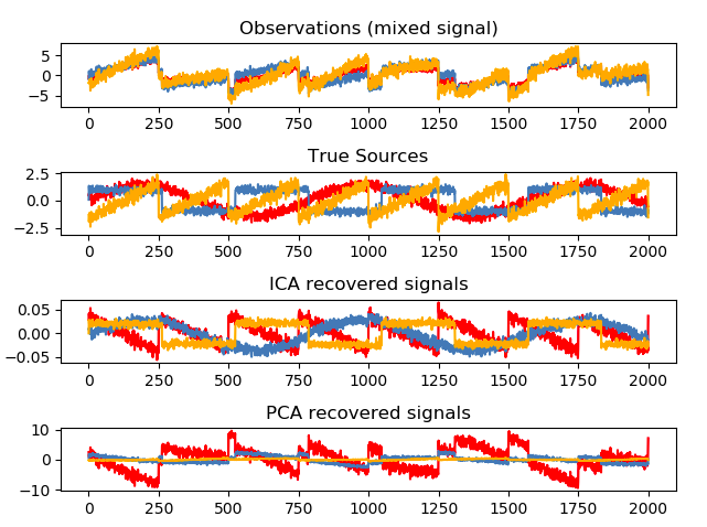
These examples assume that the mixture signals or signals that we can record are generated as a linear combination of source signals. Source signals are unknown to us, but for the sake of this example, we assume that we know the “ground truth”.
To give you more intuition about this, imagine that one of the underlying sources is actually a noise signal. The remaining signals are sine waves or sawtooth waves. Hence, the noise signal we cannot measure or remove directly.
However, if we decompose the mixture of signals and obtain the new signals in the latent space, then the noise signal can be detected! This actually was a topic of my Master thesis back in 2009!!! And for more info about this example visit the link below the image.
Next, imagine that we want to remove a saw-tooth signal from the example above. It is easy to remove it and reconstruct our original recorded signals.
Let’s explain this using a more realistic example. In the cocktail party problem, we cannot directly record only TV audio signals or remove a certain noise from the recordings. However, we can reconstruct the TV source signal in the latent space. Usually, we can then reconstruct the original signals that were present in the room. Note, that for this an important inequality must hold: the number of microphones must be larger than the number of independent sound sources.
This method is known as Blind Source Separation and it is heavily used in multi-channel signal and image processing. I hope that you will find a YouTube video tutorial amusing and helpful.
Summary
This was a bit of a theoretical post…again. However, it gave us the needed definitions and principles to frame Generative modelling problems. Sit tight! Autoencoders are just one click away and then we are going to start coding!