Highlights: The Marr-Hildreth edge detection algorithm represents one of the most elegant approaches to finding edges in images by combining Gaussian smoothing with Laplacian operations. In this comprehensive tutorial, we’ll explore how this method uses zero crossings in the second derivative to identify edges, dive into the mathematical foundations of Laplacian of Gaussian filters, and discover how separability properties make these computations remarkably efficient. Let’s begin!

 

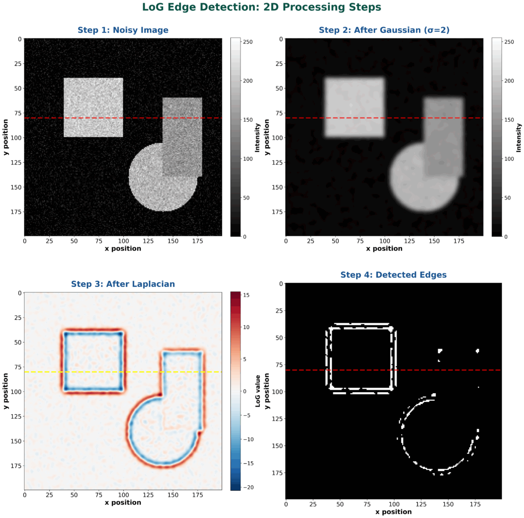
Have a look at these examples and steps! They should give you an intuition what we will talk about!

Tutorial overview:

1. Marr-Hildreth Edge Detection Fundamentals
2. Laplacian of Gaussian (LoG) Filter Implementation
3. Separability in Image Processing and Machine Learning

1. Marr-Hildreth Edge Detection Fundamentals

We will start this tutorial by explaining the Marr-Hildreth edge detector, which is historically one of the most effective edge detection algorithms.

Core Algorithm and Zero Crossing Method

Let’s begin our exploration of the Marr-Hildreth edge detector. This approach follows a systematic two-step process that’s quite elegant in its simplicity.

First, it performs smoothing using a Gaussian filter to remove noise from the image, resulting in a smoothed function \(S\). Then, it applies the Laplacian operator to this smoothed image, where the Laplacian represents the sum of second partial derivatives \(\frac{\partial^2}{\partial x^2} + \frac{\partial^2}{\partial y^2}\). This Laplacian operation is widely used across many different areas of image processing and computer vision.

$$ \text{Convolve image by Gaussian filter} \to S $$

$$ \text{Apply Laplacian to } S $$

Now, here’s where it gets interesting. The core principle behind this method lies in finding zero crossings in the Laplacian response. Remember from calculus that if the first derivative reaches a maximum, then the second derivative must equal zero at that point.

While the Sobel and other gradient-based detectors find edges by locating maxima in the first derivative, the Marr-Hildreth detector finds them by identifying zeros in the second derivative. However, there’s an important distinction between simple zeros and zero crossings – a zero crossing occurs when the function transitions from positive to negative values (or vice versa) through zero, rather than remaining constant at zero.

The algorithm scans the image systematically, examining each row and column to detect these zero crossings. When a zero crossing is identified, that location is declared an edge point. The smoothing operation uses Gaussian convolution, where we convolve the original image \(I\) with a Gaussian filter to produce the smoothed image \(S\).

The Gaussian filter is particularly effective for smoothing because of its mathematical properties, and you can visualize this as a 2D bell-shaped surface when plotted. After obtaining the smoothed image \(S\), we apply the Laplacian operator to detect the rapid intensity changes that characterize edges. Pretty neat, right?

Laplacian-Based Implementation

Building on our understanding of the zero crossing method, let’s examine how the Laplacian operation is actually implemented. When we want to find the Laplacian of a filtered image, we’re looking for the second derivative with respect to \(x\) plus the second derivative with respect to \(y\) of our smoothed image \(s\).

The process begins with our original image \(i\), to which we apply a Gaussian filter to obtain the new smoothed image \(s\). Then we compute the second derivatives in both directions and sum them up – this gives us what’s called the Laplacian of Gaussian.

$$ \Delta^2 S = \frac{\partial^2}{\partial x^2} S + \frac{\partial^2}{\partial y^2} S $$

$$ \tilde{S} = g * I \quad \text{where} \quad g = \frac{1}{\sqrt{2\pi\sigma}} e^{-\frac{r^2}{2\sigma^2}} $$

It’s important to note the conventional notation here: when you see the nabla symbol like \(\nabla\), it represents the gradient or first derivative, while \(\nabla^2\) (nabla squared) represents the Laplacian operator.

Now, here’s where the beauty of convolution theory comes into play. There are actually two equivalent ways to derive the Laplacian of Gaussian expression. The first approach is straightforward: take your image \(i\), apply Gaussian smoothing to get the filtered result, then compute the Laplacian of that smoothed image.

However, there’s a more elegant mathematical approach – we can take the Gaussian function itself and find its Laplacian by differentiating twice with respect to \(x\) and twice with respect to \(y\), then adding these second derivatives together. These two methods are theoretically identical, and you can verify this mathematically.

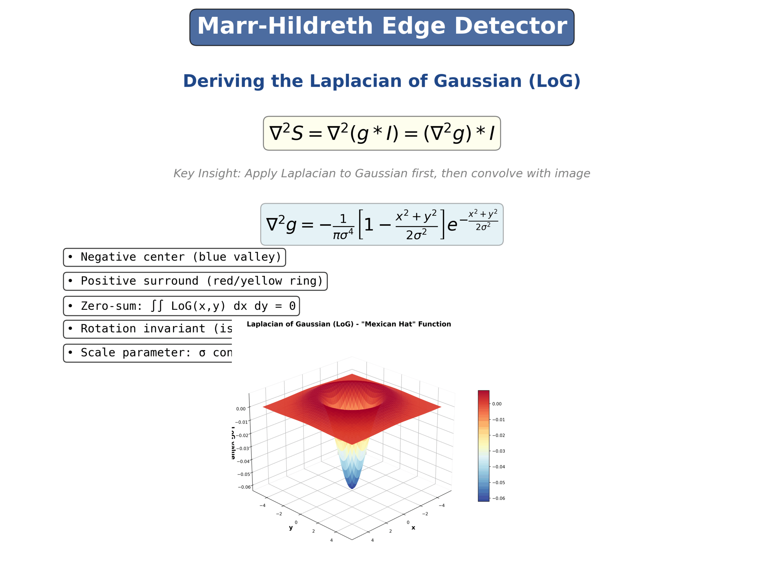
$$ \Delta^2 S = \Delta^2 (g * I) = (\Delta^2 g) * I $$

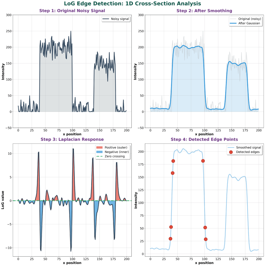
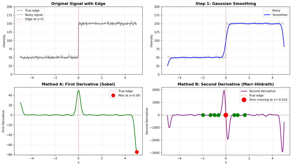
When you actually compute and plot this Laplacian of Gaussian function, you get a very distinctive shape that’s often called the “Mexican hat” function. This visualization shows the characteristic pattern with a negative peak in the center surrounded by positive values that smoothly transition around it. This inverted hat-like structure is what makes the Laplacian of Gaussian such an effective edge detector, as it responds strongly to regions where intensity changes rapidly in the image. Here, is an example of how in 1D for better insight edge detection will work. You have a noisy signal, then it is smoothed, you calculate first derivative (A), and then second derivative (B). The strong zero crossing (red point) is telling you where the edge is present. An edge in 1D can be interpreted as a pixel intensity change along a line. You can also have multiple weak zero-crossings illustrated by green points.

We can summarize all these steps visually in the Figure below. The image below is known as a Mexican hat.

Gaussian Filtering Components

Filter Parameters and Mask Configuration

Let’s start by examining the core components of Gaussian filtering, beginning with the fundamental parameter that controls everything: the standard deviation \(\sigma\). This parameter directly determines the size of the mask you’ll need to use. Have a look first at a simple 1D case – where the Gaussian function is discretized

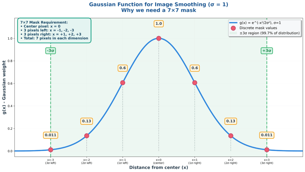
For instance, if \(\sigma = 1\), then you must have at least a 7×7 mask because the Gaussian function essentially dies out after \(3\sigma\). This means you need 3 pixels on each side of the center pixel, plus the center itself, giving you the 7×7 requirement.

Once you select your \(\sigma\) value – let’s say \(\sigma = 1\) in this case – you can calculate the corresponding values of \(g(x)\) for different positions. When \(x = 0\) (at the center), the entire expression evaluates to 1, representing the peak of the Gaussian. As you move away from center, say to \(x = 1\), the value drops to approximately 0.6, and it continues decreasing as you move further out.

This creates the characteristic bell-shaped mask of a one-dimensional Gaussian filter, which naturally extends to two dimensions.

2D Gaussian Properties and Generation

Building on our understanding of the one-dimensional case, when working with two-dimensional Gaussian distributions, we start by taking a specific value of \(\sigma\) and then evaluate the Gaussian function across different values of \(x\) and \(y\) coordinates.

This process involves plugging these coordinate values into the standard 2D Gaussian formula with our fixed \(\sigma\) parameter. To make the results practical for image processing applications, we typically multiply the computed values by a constant – often 255 – to convert them into integer values that correspond to standard image pixel intensities ranging from 0 to 255.

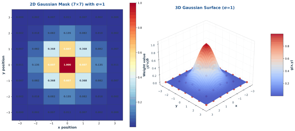
The resulting numerical values form a discrete representation of the continuous Gaussian distribution, creating what we call a Gaussian mask or kernel. This mask exhibits the characteristic properties of a 2D Gaussian: highest values at the center that gradually decrease as we move away from the center point.

The integer representation is particularly important because digital images work with discrete pixel values, making this conversion essential for practical applications in computer vision and image processing.

The ability to visualize these distributions both as numerical tables and 3D surface plots helps in understanding how the \(\sigma\) parameter controls the spread and shape of the Gaussian function.

2. Laplacian of Gaussian (LoG) Filter Implementation

LoG Filter Design and Application

Mathematical Expression and Mask Generation

Next, let’s dive into the mathematical foundation of the Laplacian of Gaussian filter and see how we can translate this continuous expression into a practical discrete mask for image processing. The LoG expression provides us with a powerful mathematical framework for edge detection and feature extraction, allowing us to generate the same type of mask that we used for the Laplacian of Gaussian operator.

The continuous Laplacian of Gaussian function can be expressed mathematically as a combination of the Laplacian operator applied to the Gaussian smoothing kernel. This gives us a filter that simultaneously smooths the image and detects edges through second derivative operations.

The mathematical beauty of the LoG filter lies in how it combines two operations – smoothing and edge detection – into a single convolution operation. Instead of first smoothing an image with a Gaussian filter and then applying the Laplacian operator separately, we can pre-compute the Laplacian of the Gaussian function itself and apply it directly to the image.

Generating the Discrete LoG Mask

To create a practical discrete LoG mask, we need to sample the continuous LoG function at discrete pixel locations. The process involves several steps that transform the elegant continuous mathematics into a working computational tool.

First, we choose our \(\sigma\) parameter, which determines both the amount of smoothing and the scale at which we detect edges. A larger \(\sigma\) creates a wider mask that detects edges at coarser scales, while a smaller \(\sigma\) creates a tighter mask sensitive to fine details.

The mask size is typically chosen to be at least \(6\sigma+1\) pixels to ensure we capture the full extent of the LoG function. For \(\sigma=1\), this gives us a 7×7 mask, while \(\sigma=2\) would require a 13×13 mask.

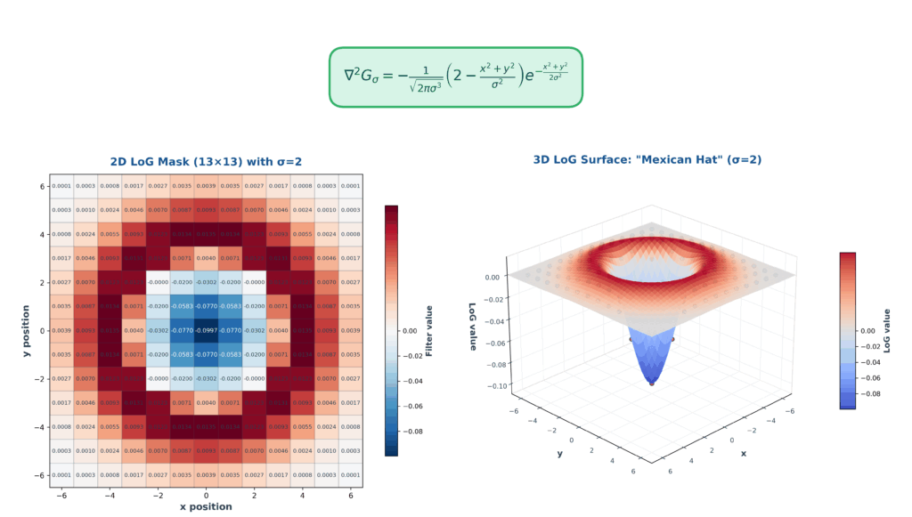
We then evaluate the LoG function at each position in this discrete grid. The function has its most negative value at the center, transitions through zero at a certain radius, and becomes positive in the outer regions.

Zero Crossing Detection Methods

Zero Crossing Fundamentals

Let me walk you through the fundamental concepts of zero crossing detection, which is really at the heart of the Marr-Hildreth edge detection algorithm. When we apply the Laplacian of Gaussian filter to an image, we’re essentially looking for points where the second derivative crosses zero – but not just any zero points, specifically points where the function transitions from positive to negative or vice versa.

The key insight here is understanding the relationship between derivatives and edge detection. In traditional edge detection methods like Sobel or Prewitt operators, we look for local maxima in the first derivative – these maxima indicate rapid intensity changes in the image. But here’s where the Marr-Hildreth approach differs elegantly: if the first derivative has a maximum at some point, then by the fundamental theorem of calculus, the second derivative must equal zero at that exact point.

This gives us two mathematically equivalent ways to find edges:

1. Find maxima in the first derivative (gradient magnitude)
2. Find zeros in the second derivative (Laplacian)

The Marr-Hildreth method chooses the second approach because it has some nice numerical properties. However, we need to be careful about what we mean by “zero.” A true zero crossing occurs when the function actually crosses through zero, changing sign from positive to negative or negative to positive. This is different from a point where the function merely touches zero and continues in the same direction, or where it remains at zero for an extended region. Have a look again at the red point vs the green points in the image below.

Implementation and Detection Techniques

Now let’s dive into the practical implementation of zero crossing detection. The algorithm systematically scans the filtered image, examining each pixel and its neighbors to identify potential zero crossings. There are several approaches to this detection, each with its own trade-offs.

The most straightforward method examines the signs of neighboring pixels. For each pixel, we check if any of its 4-connected or 8-connected neighbors has an opposite sign. If we find pixels of opposite signs adjacent to each other, we know a zero crossing must exist between them. This is the most computationally efficient approach, though it can be sensitive to noise.

A more sophisticated approach involves examining not just the sign change, but also the magnitude of the values on either side of the crossing. The slope or steepness of the zero crossing gives us information about the edge strength. A steep zero crossing (large magnitude change) indicates a strong edge, while a shallow crossing might indicate a weak edge or noise. We can use this information to threshold our edge detection, keeping only the most significant edges.

The edge strength at a zero crossing can be quantified by measuring the absolute difference between the neighboring pixels of opposite sign:

$$ \text{Edge Strength} = |L(x_1, y_1) – L(x_2, y_2)| $$

where \(L(x_1, y_1)\) and \(L(x_2, y_2)\) are the Laplacian values at neighboring pixels with opposite signs.

Some implementations also use interpolation to find the precise sub-pixel location of the zero crossing. Since we’re working with discrete pixels, the actual zero crossing might occur somewhere between two pixel locations. By fitting a line between the two neighboring pixels of opposite sign, we can estimate the exact position where the Laplacian equals zero, giving us sub-pixel accuracy in edge localization.

Discrete LoG Filter Construction

Continuous to Discrete Transformation

The transition from continuous mathematical expressions to discrete implementations is where theory meets practice in image processing. When working with the Laplacian of Gaussian (LoG) filter, we need to carefully convert our beautiful continuous equations into practical discrete masks that can be applied to digital images.

Let’s start with the continuous Laplacian of Gaussian function. In its most general form, the 2D Gaussian is expressed as:

$$ g(x,y) = \frac{1}{2\pi\sigma^2} e^{-\frac{x^2 + y^2}{2\sigma^2}} $$

The Laplacian operator \(\nabla^2\) applied to this Gaussian gives us:

$$ \nabla^2 g(x,y) = \frac{\partial^2 g}{\partial x^2} + \frac{\partial^2 g}{\partial y^2} $$

When we compute these second partial derivatives and simplify, we get the complete Laplacian of Gaussian expression:

$$ \nabla^2 g(x,y) = -\frac{1}{\pi\sigma^4}\left[1 – \frac{x^2 + y^2}{2\sigma^2}\right] e^{-\frac{x^2 + y^2}{2\sigma^2}} $$

This continuous function needs to be sampled at discrete pixel locations to create our filter mask. The process involves evaluating the LoG function at integer coordinates corresponding to the mask positions. For example, with \(\sigma = 1\), we typically use a 7×7 mask centered at the origin, evaluating the function at points like (0,0), (0,1), (1,0), (1,1), and so on.

Discrete Mask Generation and Values

Now let’s get practical and see how we actually generate these discrete mask values. The process is systematic: we choose our \(\sigma\) value, determine the appropriate mask size (remember, at least \(6\sigma+1\) pixels for full coverage), then compute the LoG value at each mask position.

Let me show you a concrete example. For \(\sigma = 1\), the center of a 7×7 LoG mask will have the maximum negative value because \(x^2 + y^2 = 0\) at the origin. As we move away from the center, the values first remain negative, then cross through zero, and finally become positive at the outer edges.

A typical 7×7 LoG mask with \(\sigma = 1\) looks something like this in structure (showing approximate values):

 0   0   1   1   1   0   0
 0   1   3   3   3   1   0
 1   3   0  -7   0   3   1
 1   3  -7 -24  -7   3   1
 1   3   0  -7   0   3   1
 0   1   3   3   3   1   0
 0   0   1   1   1   0   0

The actual values will sum to approximately zero (or be normalized to sum to zero), which is an important property for preserving image brightness. The central negative region is surrounded by a positive ring, creating the characteristic “Mexican hat” cross-section.

The mask generation process follows these steps:

1. Choose \(\sigma\) and calculate mask size: \(n = 2 \cdot \lceil 3\sigma \rceil + 1\)
2. For each position (i,j) in the mask, calculate \(x = i – \text{center}\) and \(y = j – \text{center}\)
3. Evaluate \(\nabla^2 g(x,y)\) using the LoG formula
4. Optionally normalize the mask so the sum equals zero
5. Store the values in the discrete mask array

This discrete representation can then be convolved with our image to detect edges through zero crossing detection, bringing together all the theoretical concepts we’ve discussed into a practical edge detection system.

LoG Filter Properties and Characteristics

Scale-Space Representation

One of the most powerful aspects of the Laplacian of Gaussian filter is its relationship to scale-space theory, a fundamental concept in computer vision. The \(\sigma\) parameter doesn’t just control the smoothing amount – it actually determines the spatial scale at which we’re analyzing the image structure.

Different values of \(\sigma\) allow us to detect edges at different scales. A small \(\sigma\) (say, 0.5 or 1.0) will respond to fine details and sharp transitions in the image – think of individual texture elements or thin lines. A larger \(\sigma\) (like 3.0 or 5.0) smooths out fine details and responds only to broader, more significant intensity changes – major boundaries between large regions.

This multi-scale nature is incredibly useful because edges exist at different scales in natural images. The boundary between a person and the background is a large-scale edge, while the texture of fabric or hair represents fine-scale edges. By applying LoG filters with different \(\sigma\) values, we can build a complete scale-space representation of the image.

The mathematical elegance here is that as we increase \(\sigma\), we’re not just blurring more – we’re actually moving up in a hierarchy of image structure. This scale-space approach is fundamental to many modern computer vision algorithms, including SIFT features, blob detection, and even deep learning architectures that use progressively larger receptive fields.

Rotation Invariance and Isotropy

Another beautiful property of the Laplacian of Gaussian filter is its rotational invariance or isotropy. What this means is that the filter responds equally to edges regardless of their orientation in the image. This is in stark contrast to gradient-based operators like Sobel, which have different responses for horizontal versus vertical edges.

The mathematical reason for this isotropy comes from the circular symmetry of both the Gaussian function and the Laplacian operator. The Gaussian depends only on the distance from the center \(r = \sqrt{x^2 + y^2}\), not on the angle. Similarly, the Laplacian operator treats the \(x\) and \(y\) directions equally.

This means that a vertical edge, horizontal edge, or diagonal edge of the same strength will all produce zero crossings of equal magnitude. This property makes LoG-based edge detection very robust and fair across all orientations, which is particularly valuable in applications where edges may appear at arbitrary angles.

However, this isotropy comes with a trade-off: we lose information about edge direction. If you need to know the orientation of edges (for instance, to compute image gradients or flow fields), you’ll need to supplement LoG detection with gradient direction computation. But for pure edge localization, the rotation invariance is a significant advantage that simplifies both the algorithm and the interpretation of results.

Implementation Efficiency and Optimization

Separability-Based Optimization

Now, let’s discuss one of the most important computational optimizations in image processing: leveraging the separability of Gaussian filters. This technique can dramatically reduce the computational cost of applying Laplacian of Gaussian filters to images.

As we discussed earlier, a 2D Gaussian filter can be separated into two 1D filters:

$$ g(x,y) = g(x) \cdot g(y) $$

This gives us the same result as a two-dimensional Gaussian filter \(g(x,y)\), but using only two one-dimensional convolutions instead of one computationally expensive two-dimensional operation.

For Laplacian Gaussian filtering, the separability approach becomes more complex but remains advantageous. We start with the original image and apply the Gaussian second derivative in one dimension, followed by the regular Gaussian in the \(y\) direction.

$$ \Delta^2 S = (I * g_{xx}(x)) * g(y) + (I * g_{yy}(y)) * g(x) $$

Then we take the same original image and apply the second-derivative Gaussian in the \(y\) direction (along columns), followed by the regular Gaussian in the \(x\) direction (along each row of the result). Finally, we add these two results together to obtain the complete Laplacian Gaussian response.

This separable approach to Laplacian Gaussian filtering requires a maximum of four convolutions: first convolution applies \(g_{xx}(x)\), second convolution applies \(g(y)\), third convolution applies \(g_{yy}(y)\), and fourth convolution applies \(g(x)\).

While this isn’t as efficient as the simple two-convolution Gaussian case, it still provides substantial computational savings compared to direct two-dimensional Laplacian Gaussian filtering, demonstrating the practical value of leveraging separability properties in image processing operations.

3. Separability in Image Processing and Machine Learning

Gaussian Filter Separability

Separable Gaussian Filtering Applications

Now that we understand the theoretical foundation of Gaussian filter separability, let’s explore how this property enables powerful computational approaches in practice. When working with separable Gaussian filtering, we can leverage the mathematical properties of the Laplacian operator to create more efficient computational approaches.

The key insight is that the Laplacian of a smoothed image \(S\) can be expressed as the convolution of the original image \(I\) with the Laplacian of the Gaussian kernel \(g\).

$$ \Delta^2 S = \Delta^2 (g * I) = (\Delta^2 g) * I = I * (\Delta^2 g) $$

This mathematical relationship becomes particularly powerful when we consider the separable nature of Gaussian kernels. Since we can decompose the 2D Gaussian into separate \(x\) and \(y\) components, the Laplacian operation can be similarly decomposed. This allows us to compute the second derivatives \(g_{xx}(x)\) and \(g_{yy}(y)\) independently, leading to significant computational savings.

$$ \Delta^2 S = (I * g_{xx}(x)) * g(x) + (I * g_{yy}(y)) * g(y) $$

The practical applications of this separable approach are extensive in computer vision and image processing. By breaking down the filtering operation into separate horizontal and vertical passes, we can achieve the same results as a full 2D convolution but with dramatically reduced computational complexity.

This technique is fundamental in edge detection algorithms, blob detection, and multi-scale image analysis, where the efficiency gains become crucial when processing large images or real-time video streams.

Machine Learning Classification Separability

Classification Problem Separability

When we talk about machine learning classification, one of the most fundamental concepts we need to understand is separability – essentially, how well we can distinguish between different classes in our data. As we examine these filtering processes, there’s an important relationship between how we process images and how we approach classification problems.

Looking at these flow diagrams, we can see the fundamental differences in processing approaches. The comparison between standard Gaussian filtering and Laplacian of Gaussian filtering reveals how different mathematical operations can lead to different computational pathways.

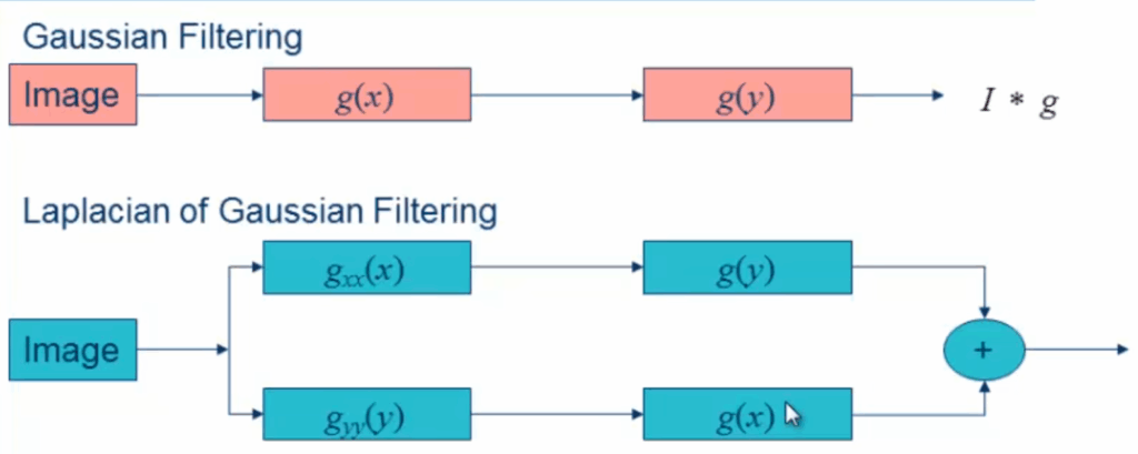
The comparison between these two filtering approaches reveals the fundamental differences in how we process images through Gaussian-based operations. The standard Gaussian filtering follows a straightforward path with filter functions \(g(x)\) and \(g(y)\), while the Laplacian of Gaussian variant introduces the \(g_{xx}(x)\) operation that modifies the processing pathway significantly.

Understanding these processing differences is crucial for determining how separable our classification problems will be. The sequential steps from input image through the various filtering operations, ultimately leading to the convolution result \(I * g\), must be clearly understood to make informed decisions about which approach we’re implementing in our classification systems.

This relationship between image processing separability and machine learning classification separability demonstrates how fundamental mathematical concepts apply across different domains of computer science and engineering.

Summary

In this comprehensive exploration of Marr-Hildreth edge detection, we’ve covered the fundamental principles that make this algorithm so effective in computer vision applications. We began by understanding how the two-step process of Gaussian smoothing followed by Laplacian operation creates a powerful edge detection framework through zero crossing identification. The mathematical elegance of finding edges in the second derivative rather than the first derivative provides a robust approach to boundary detection that has stood the test of time.

We then delved deep into the Laplacian of Gaussian filter implementation, exploring how the continuous mathematical expressions translate into practical discrete masks for image processing. The zero crossing detection techniques we examined show how to not only identify edge locations but also measure their strength, providing a complete framework for robust edge detection. The separability analysis revealed one of the most important computational optimizations in image processing – the ability to decompose 2D operations into efficient 1D convolutions, reducing computational complexity from \(n^2\) to \(4n\) operations.

Looking forward, these concepts form the foundation for more advanced computer vision techniques including multi-scale edge detection, feature extraction, and modern deep learning approaches to image analysis. The mathematical principles of separability and zero crossing detection continue to influence contemporary algorithms, making this classical approach as relevant today as it was when first developed. Understanding these fundamentals provides the essential groundwork for tackling more complex challenges in computer vision and image processing.