Why Agent Context Explodes — Quadratic Growth, Serving Costs, and Efficient Attention (Linear, DeltaNet, KDA, MLA)

Highlights: Graham Neubig’s lecture in the CMU 11-768 AI Agents course (Fall 2026) looks at why agent context grows quadratically and what architectures make long context affordable to serve. We walk through the token composition of real OpenHands sessions, the prefill/decode split and its serving metrics, and the local, linear, sparse and KV-compression mechanisms used in current frontier models. This post covers roughly the first 35 minutes of the lecture; training, positional encodings, caching and compaction follow in a second part.

• Quadratic history growth: With a 1K system prompt and 5K tokens per call, per-call inputs run 6K, 11K, 16K, 21K, 26K, and the cumulative processed input reaches 80K tokens after only five turns.
• Where the tokens go: Across 1,500 OpenHands sessions averaging 78K tokens, 37% were tool results, 23% system prompt and tool descriptions, 20% tool calls, 9% user messages, 9% reasoning traces, and 2% model replies.
• Capacity vs. efficiency: Needle-in-a-haystack, RULER and HELMET show effective context degrading well before the advertised limit, while serving splits into compute-bound prefill and sequential, memory-bound decode.
• Serving metrics and provider spread: Time to first token, time per output token and throughput vary sharply in practice, from a Mistral endpoint at 3 tokens per second to hundreds of tokens per second on providers such as CoreWeave (OpenRouter data for GLM-5.2).
• Capping comparisons per step: Sliding-window masking turns O(n²) into O(wn), while dropping the softmax lets linear attention collapse history into a fixed-size state S_t = S_{t-1} + k_t v_tᵀ, extended by DeltaNet, Gated DeltaNet and Kimi Delta Attention.
• Hybrids and KV compression: Qwen3.8-Flash-Next, GLM-5.3-Flash, Kimi K3, Nemotron 3 Ultra, Inkling-Small and DeepSeek-V4-Pro-0813 all interleave local layers with periodic global or sparse ones, alongside GQA and Multi-Head Latent Attention to shrink the KV cache.

Tutorial Overview:

1. Context Management and Quadratic History Scaling in Agents
2. Empirical Token Composition Across Real-World Agent Sessions
3. Retrieval Capacity Degradation and Effective Context Limits
4. LLM Inference Mechanics: Prefill vs. Decode Execution
5. Serving Performance Metrics: Latency Dynamics and Throughput
6. Real-World Provider Divergence and Cost Dynamics
7. The Quadratic Bottleneck of Standard Causal Attention
8. Local Modeling: Reducing Pairwise Costs Linearly
9. Modern Hybrid Architectures Combining Local and Periodic Global Layers
10. Sliding-Window Attention with Causal Window Masking
11. From Softmax to a Constant-Size Recurrent State
12. Targeted Updates and Gated Retention in Recurrent Attention
13. Sparse Attention: Fixed Topologies vs. Dynamic Content Routing
14. KV Cache Compression: From MHA/MQA/GQA to Multi-Head Latent Attention
15. Summary

A note on scope: this post covers how agent context grows, how inference and serving work, and the architectures that make long context affordable (roughly the first 35 minutes of the lecture); training curricula, positional encodings (RoPE/NoPE/YaRN), prompt and KV caching, and compaction are covered in a second part.

---

1. Context Management and Quadratic History Scaling in Agents

Context management for long-context agents overlaps heavily with general context management for large language models (LLMs) — the foundational theory is the same. But long context matters far more once you build autonomous agents, and it is rarely covered well in standard prerequisite courses. So we will look at the specialized long-context architectures used in state-of-the-art open models, and at the best practices the community relies on to manage huge context windows.

Why is this so pressing? Because an agent’s context grows fast. In a typical agent loop, the total volume of token accesses scales quadratically as a direct consequence of linear history growth. Say you start with a 1K-token fixed prefix (system prompt and tool definitions) and every call adds another 5K tokens of history: the first call processes 6K tokens, the second 11K, then 16K, 21K and 26K.

1.1 Quadratic Token Accumulation from Linear Turns

Picture how memory fills across sequential calls. Call 1 occupies 6K tokens of the context window, giving a cumulative total of 6K. The per-call input then grows to 11K tokens in Call 2 and 16K in Call 3, pushing the cumulative totals from 6K to 17K to 33K tokens — linear interaction turns, quadratic context accumulation.

At any execution step (t), the total input fed into the model follows a compounding sequence:

[\text{input}_t = \text{fixed prefix} + \text{history before call } t]

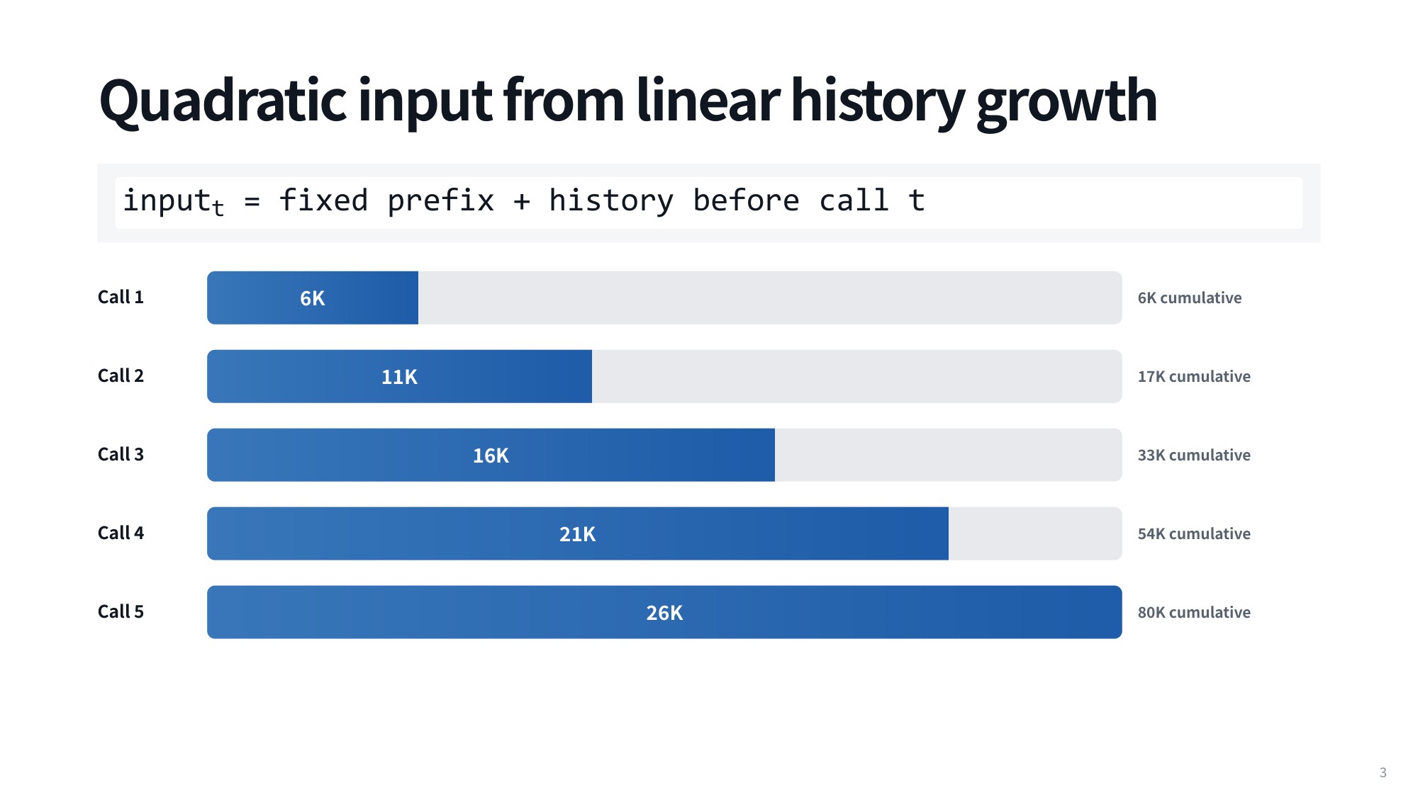
Fig 1. Quadratic input from linear history growth

1.2 Prompt Expansion Across Execution Steps

Run the agent loop naively — re-ingesting the full context every turn — and you process 80K tokens across just five turns. The prompt widens at every step because each input carries the complete historical log of prior thoughts, tool calls, and environment responses on top of the fixed system prefix.

Real workflows do not stop after a handful of steps; they can run continuously for long stretches. In the CMU lecture, Graham Neubig notes that while the longest recorded single coding-agent session is hard to pin down, he has run sessions spanning multiple days and worked alongside an agent for nearly an entire working day. The accumulated context becomes enormous, and the real cost is steeper than the token counts suggest, since attention complexity scales quadratically with sequence length.

It is easy to take real-time responsiveness for granted with tools like Claude Code or Codex. Delivering it means evaluating a multi-trillion parameter model repeatedly within seconds — an extraordinary engineering feat. By Neubig’s estimate, Codex alone has around 25 million daily users. Multiply that by queries arriving every few seconds against a model of that size, and the computational challenge of quadratic history growth becomes impossible to ignore.

---

2. Empirical Token Composition Across Real-World Agent Sessions

2.1 Where OpenHands Sessions Spend Their Tokens

Why do agent prompts grow so fast? In the CMU lecture, Graham Neubig breaks down the prompt composition of 1,500 sessions from the OpenHands coding agent. These were short sessions involving single tasks, not the multi-day runs users sometimes launch, and yet each one consumed about 78,000 tokens on average.

Of that total, 23% went to the system prompt and its tool descriptions. That is a hefty footprint for a coding agent: the OpenHands system prompt runs somewhere around 15,000 to 18,000 tokens, because the agent is highly opinionated about how work should be done. Across different setups, such prompts range from 8,000 to 20,000 tokens depending on factors like how many tools are loaded into the environment.

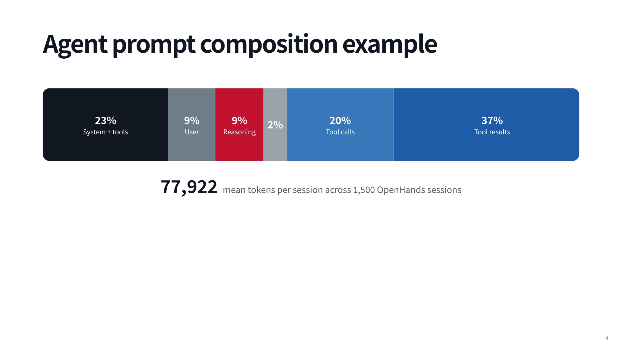
Fig 2. Agent prompt composition example

Human conversation is a small slice. User messages — the initial task plus later follow-ups — accounted for 9% of tokens, and reasoning traces, where the model thinks through the problem, another 9%. Model replies addressed directly to the user made up only 2%. The model burns roughly five times as many tokens reasoning internally as it does talking to you.

Everything else is environment interaction: 20% of tokens were tool calls such as writing or reading code, and 37% were tool results, like the contents of a file that was read. Every step in an execution trajectory contributes all of these pieces, so context piles up quickly. Environment feedback and system scaffolding, not conversational turn-taking, are what fill an agent’s window.

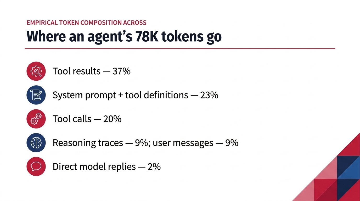
Fig 3. Where an agent’s 78K tokens go

---

3. Retrieval Capacity Degradation and Effective Context Limits

3.1 Capacity vs. Serving Efficiency

Once you start handling very long context, two challenges show up immediately. The first is capacity: is the model genuinely able to use that much evidence at all? Training models to process extremely long contexts effectively is notoriously hard.

Getting capacity right means getting several interconnected pieces right: the model architecture, the positional encodings, high-quality training data, and evaluation methods robust enough to tell you whether the model actually performs well at scale.

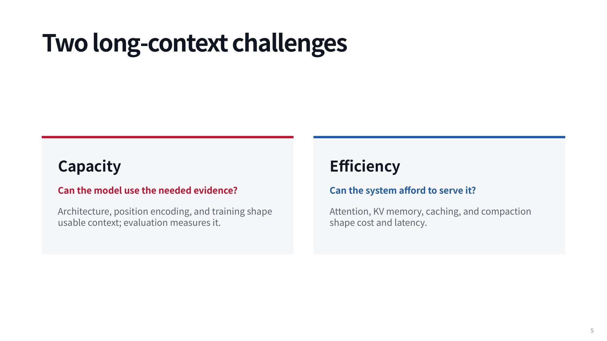
Fig 4. Two long-context challenges: can the model use the evidence (capacity), and can the system afford to serve it (efficiency)?

The second challenge is efficiency: can the infrastructure afford to serve models running over these massive contexts? A wide range of specialized engineering techniques exist to carry that operational burden.

At inference time, execution splits into prefill and decode stages — computing representations for the input prompt, then generating new tokens step by step. On top of that come the operational decisions: scheduling many concurrent user queries, and storing intermediate key and value states in the KV cache so they can be reused across generation steps instead of recomputed from scratch.

3.2 Advertised vs. Effective Context Length

The quadratic attention cost makes efficiency a steep bottleneck. But solving the serving problem still leaves you facing the effectiveness side of the equation.

A model (or an optimized serving stack) that accepts a million tokens in its prompt window does not necessarily use those million tokens well.

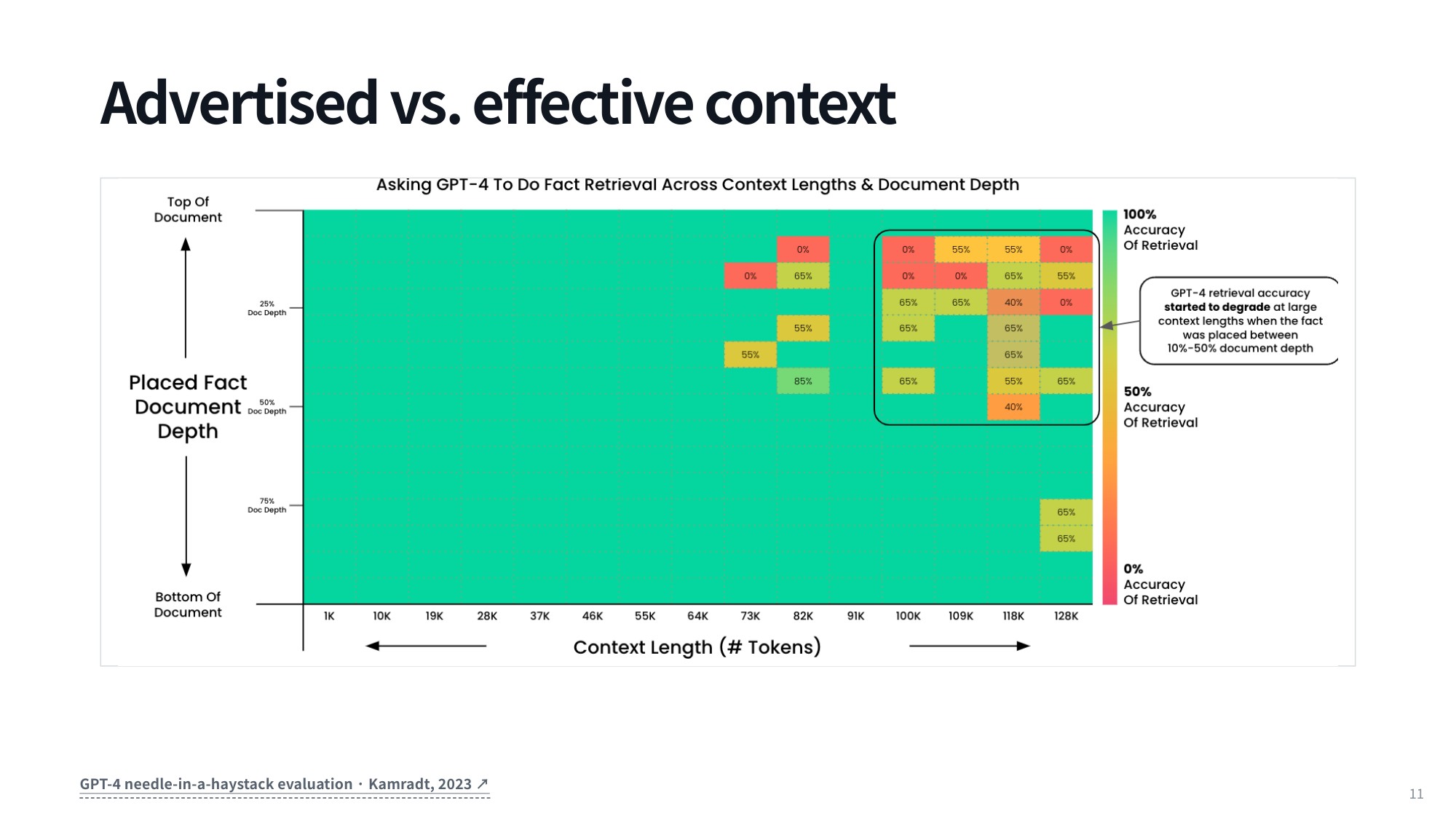
Fig 5. Advertised vs. effective context: GPT-4 needle-in-a-haystack results (Kamradt, 2023)

The classic way to probe that gap is the needle-in-a-haystack evaluation, and its setup is deliberately odd. The creators collected a large body of essays by Paul Graham, the entrepreneur and co-founder of Y Combinator, and inserted one random sentence deep inside them — something mundane, such as naming the best place in San Francisco to eat a sandwich.

3.3 Degradation in Extended Agent Workloads

With the synthetic “needle” buried in the text “haystack,” you ask the model: “Where is the best place in San Francisco to eat a sandwich?” It has to locate that isolated snippet and answer from the provided context.

Researchers then push the surrounding context longer and longer. Weaker models start degrading, showing a clear drop-off in their ability to retrieve the fact from very long contexts. Plenty of realistic benchmarks capture the same degradation across real tasks, with RULER and HELMET among the most widely used today. The takeaway: an architecture that technically supports a huge context window can still see performance plummet as context grows.

Have you hit this yourself with a coding agent or any long-running autonomous agent? The failure modes are familiar. The system gradually forgets earlier conversational turns, or it forgets the system instructions and constraints you set at the very start.

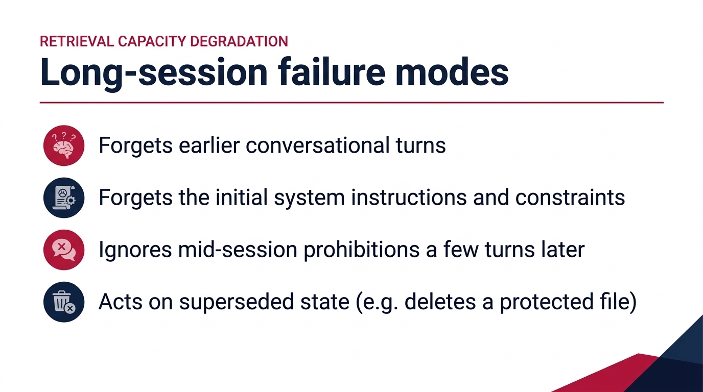
Fig 6. Long-session failure modes

In the CMU lecture, Graham Neubig describes telling an agent mid-session not to do something and watching it do exactly that a few turns later. One widely discussed example makes the point sharply: a user explicitly wrote “Do not delete this,” and the agent deleted the target file anyway, having lost track of the instruction in the accumulated context. That is a serious problem for agentic applications, where users supply critical instructions incrementally throughout the workflow.

---

4. LLM Inference Mechanics: Prefill vs. Decode Execution

4.1 Compute-Bound Prefill vs. Memory-Bound Decode

To understand why we avoid recomputing things from scratch, we need the two distinct phases of language model inference. The first is prefill (sometimes called encoding, though prefill is the term of art these days): you take all the input tokens you do not need to generate and compute the corresponding key and value pairs for each of them.

In a serving stack, a request first hits a scheduler that queues, batches and routes it. Prefill and decode then share one persistent per-request KV cache.

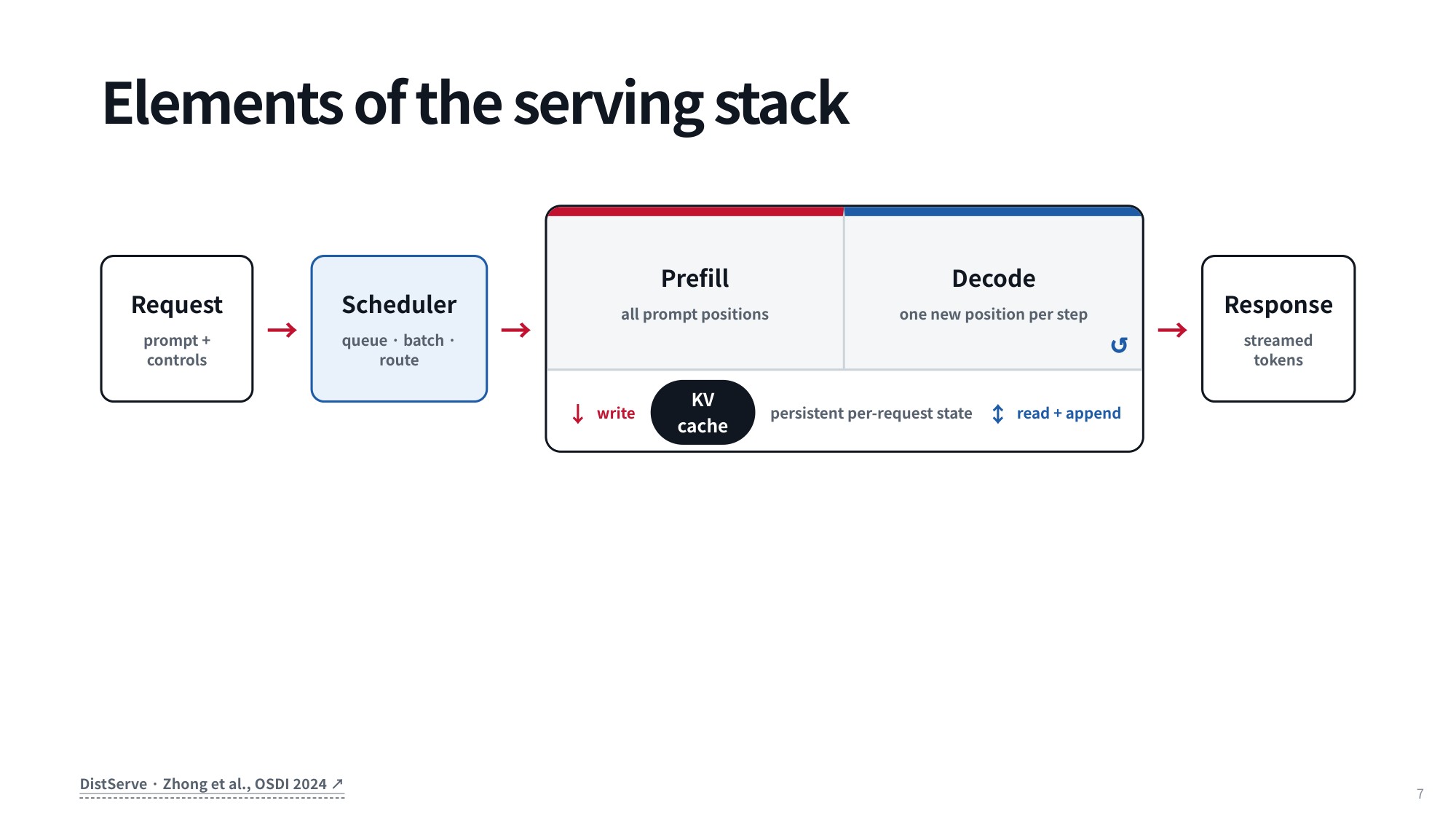
Fig 7. Request → scheduler → prefill/decode with a persistent per-request KV cache (DistServe, Zhong et al., OSDI 2024)

The operationally crucial point about prefill is that it runs across the whole sequence in a batched, parallel fashion. Since every input token is known upfront, the hardware can process them concurrently.

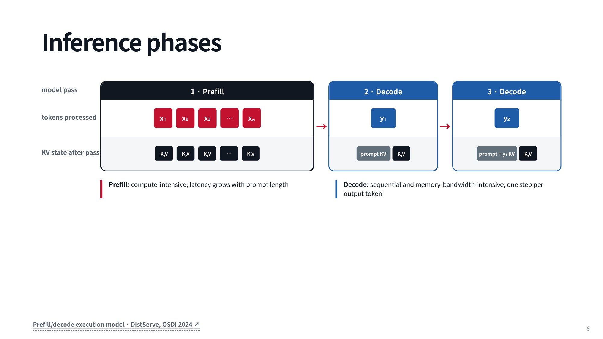
Fig 8. The two inference phases: prefill computes all prompt positions at once, while decode adds one new position per step

The decode phase works completely differently. You take the prompt and its accumulated key-value pairs, generate an output token, and append that token’s newly computed key-value pair back into the cache — incrementally, one token at a time. This sequential, autoregressive process stands in stark contrast to prefill, which runs in batch.

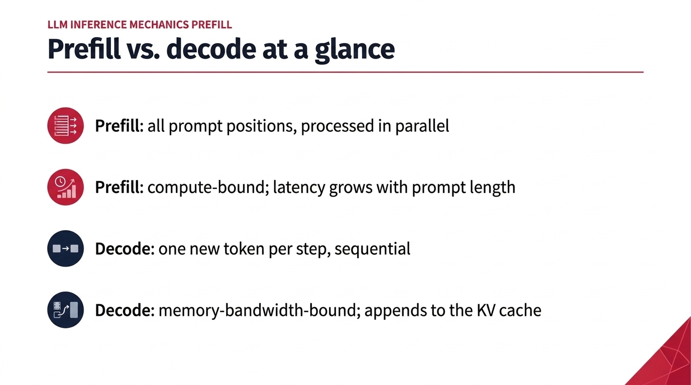
Fig 9. Prefill vs. decode at a glance

4.2 Serving Trade-Offs for Agent Workloads

This split between batched prefill and token-by-token decode underpins the serving metrics we monitor in production. Which ones matter depends entirely on how the agent is deployed. In an interactive task inside your favorite coding CLI, you care intensely about Time to First Token (TTFT) and Time Per Output Token (TPOT) to keep the loop responsive. If instead you run an agent in the background on tasks that finish overnight, those latency numbers may not matter at all.

That leaves real engineering trade-offs between throughput, cost, and how fast tokens arrive. In the CMU lecture, Graham Neubig notes that inference providers serving coding agents routinely ask which metric the customer cares about more, so they can tune the serving system for that target. There are concrete ways to make those optimizations.

---

5. Serving Performance Metrics: Latency Dynamics and Throughput

5.1 TTFT and Time Per Output Token

Once we judge an architecture from the viewpoint of a real serving system, we need concrete numbers. The first is Time to First Token (TTFT): how long you wait between submitting a query and seeing the very first token appear.

You have felt this if you use ChatGPT. A long prompt takes noticeably longer to start responding than a short one, because a larger input context demands much more computation up front in the prefill phase, which drives TTFT up.

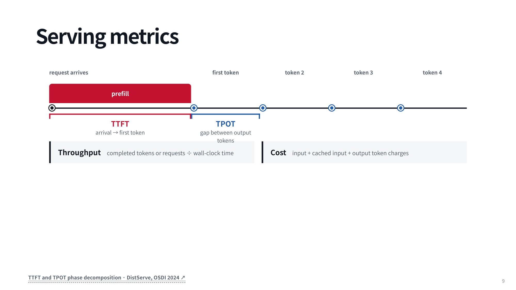
Fig 10. Serving metrics

The second metric is Time Per Output Token (TPOT), the time needed to generate each subsequent token during decoding. The speed numbers reported on benchmarking platforms like OpenRouter usually correspond to this.

Those published figures ignore the prefill stage and capture only the steady-state pacing between tokens as they stream back. Compare hosting providers for GLM-5.2 on OpenRouter and the variance is large: depending on infrastructure, you see 63, 48, and 24 tokens per second across setups.

5.2 Throughput and Concurrency in Production

In production, these latencies play out across an end-to-end timeline. A serving diagram tracks the full lifecycle of a request: arrival, prefill, TTFT, then TPOT for every token generated afterwards.

Mapping that sequence is the foundation for evaluating overall throughput and managing concurrency across many simultaneous users.

5.3 The Cost of Serving Tokens

Throughput is defined as the total number of completed tokens across all requests divided by total wall clock time. Since it aggregates concurrent workloads, it is evaluated holistically across the entire serving cluster.

And the economics follow directly from it: how much money does it cost you to serve those tokens at scale?

---

6. Real-World Provider Divergence and Cost Dynamics

6.1 Latency and Throughput Vary by Provider

The same model served by two different hosts can behave like two different products. Inspect any live routing endpoint and the gap in empirical throughput jumps out immediately.

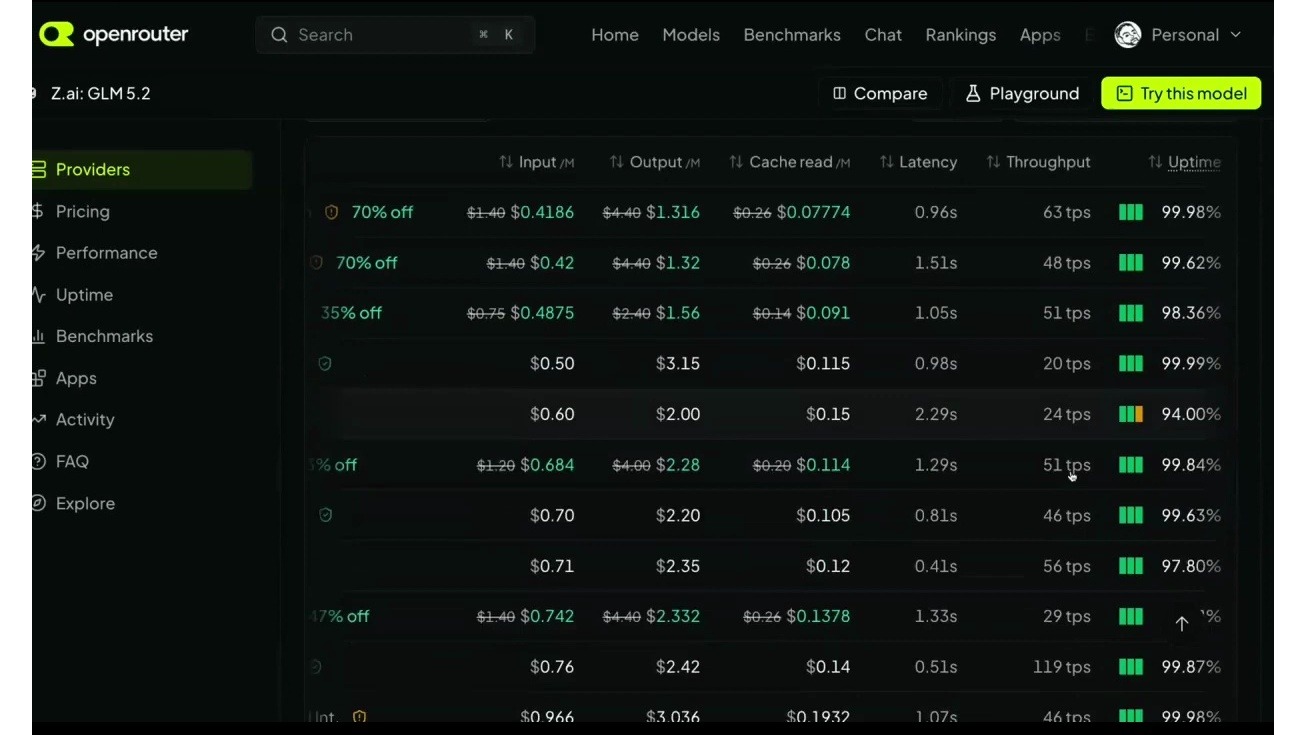
Fig 11. OpenRouter dashboard comparing provider pricing, latency, throughput, and uptime metrics

6.2 What the OpenRouter Numbers Show

On OpenRouter, one Mistral endpoint for GLM-5.2 was delivering only 3 tokens per second, while other providers on the same list, such as CoreWeave, were reaching hundreds of tokens per second. Same model, same list: the spread comes entirely from who is hosting it.

6.3 Pricing and Prompt Caching Discounts

Token pricing and prompt caching discounts differ just as much across endpoints. For long-context workloads those differences compound quickly, so your choice of provider shapes both the cost and the user experience of your agent.

---

7. The Quadratic Bottleneck of Standard Causal Attention

7.1 Causal Masking and Attention Notation

Let’s fix notation before we talk about cost. We represent the input sequence as a matrix (X \in \mathbb{R}^{n \times d}), where each row is a token-state representation (z_t). Projection weight matrices turn it into the query, key, and value matrices (Q), (K), and (V). Lowercase (q_i), (k_j), and (v_j) denote row vectors of those matrices, and (d_k) is the key width.

The linear projections are:

[Q = XW_Q, \quad K = XW_K, \quad V = XW_V]

From there, we take the dot product between queries and keys, scale it by (\sqrt{d_k}), and add the causal mask (M) to the scaled scores. A softmax over the scaled scores gives the normalized attention matrix (A), and multiplying by (V) yields the output (O):

[A = \text{softmax}\left(\frac{QK^\top}{\sqrt{d_k}} + M\right), \quad O = AV]

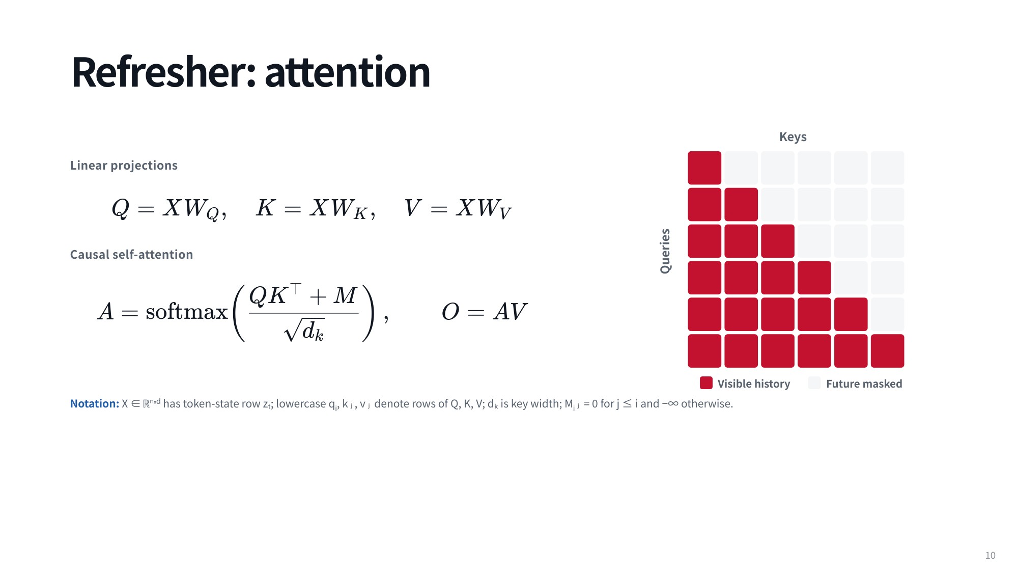
Fig 12. Refresher: attention

In an autoregressive model, causal full attention lets every token see the current and all previous positions while masking the future. That is implemented with the additive mask (M), where (M_{i, j} = 0) whenever (j \le i) and (M_{i, j} = -\infty) otherwise, blocking attention to later tokens entirely. Since every token attends back to all earlier positions, we pay for pairwise comparisons across the whole visible sequence.

7.2 Global Pairwise Comparisons

Standard causal attention is global: it compares every token with every other visible token, which means quadratic complexity. Modern state-of-the-art models advertise context lengths from 256k up to a million tokens, and most teams are pushing for a million, because nobody wants to ship the model capped at 256k when competitors offer a million.

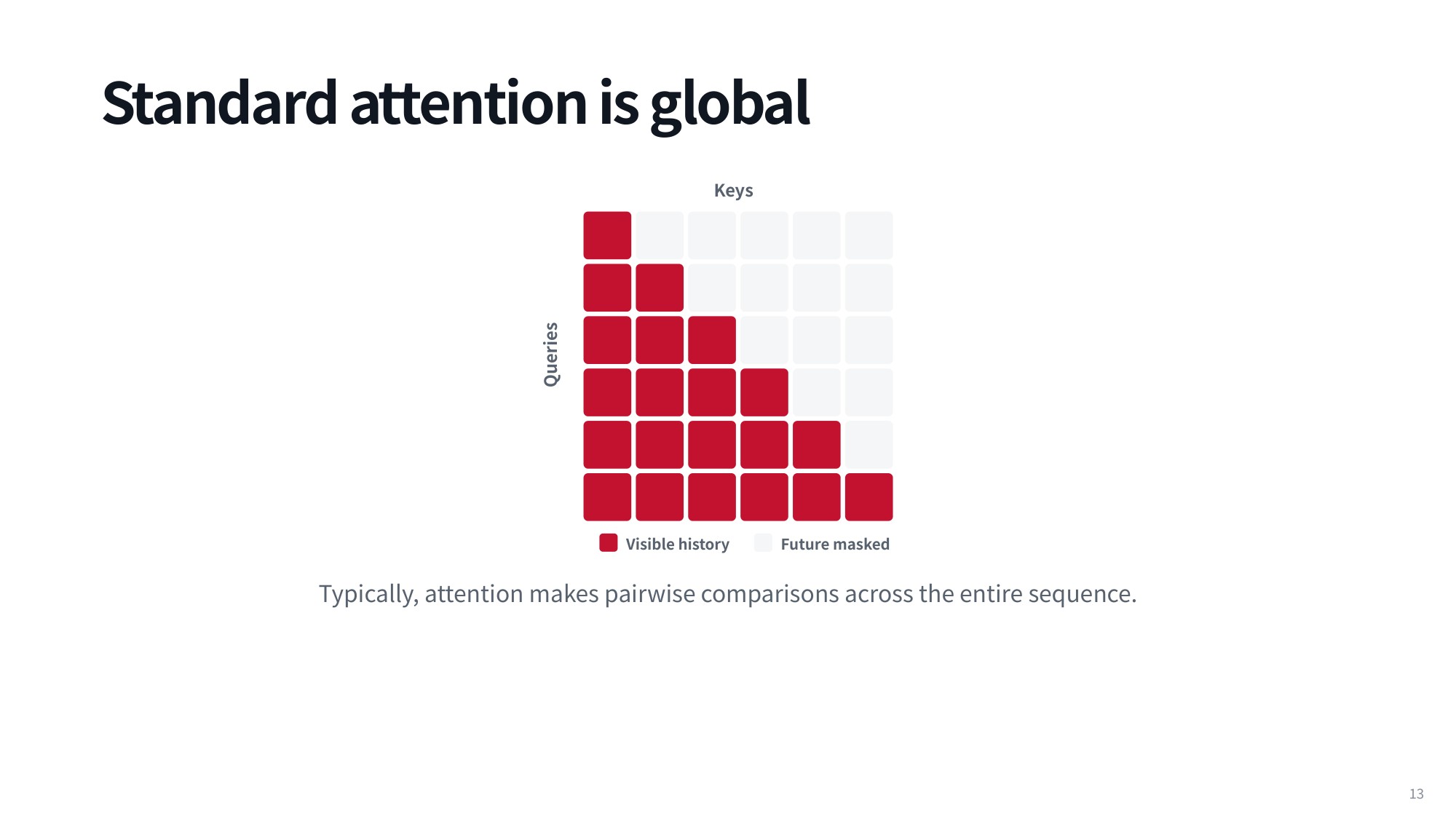
Fig 13. Standard attention is global

At a million tokens, the number of pairwise comparisons reaches (10^{12}) — a full trillion comparisons for a single sequence. Attention matrices of that size put a relentless load on hardware.

And each comparison is not a cheap scalar operation; it multiplies large vectors together, again and again. Factoring in the vector dimensions across all those interactions, the total climbs to roughly (10^{20}) operations for one sequence, which is the real severity of quadratic scaling.

---

8. Local Modeling: Reducing Pairwise Costs Linearly

8.1 Restricting Attention to a Local Window

How do we escape the quadratic bottleneck? Nearly every practical answer works the same way: cap the number of comparisons each token is allowed to make at every time step. Instead of letting attention grow without bound, we fix its span.

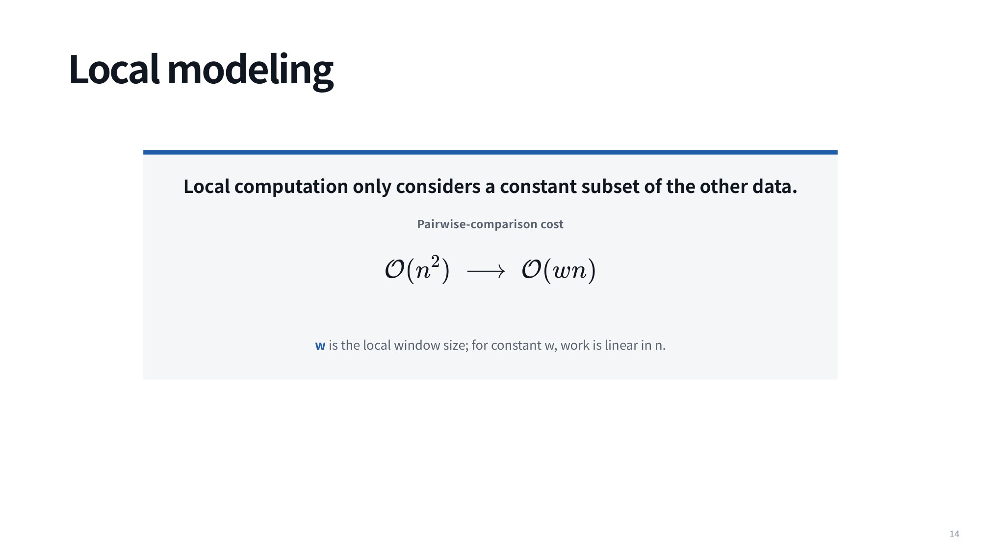
Fig 14. Local modeling: the pairwise-comparison cost falls from O(n²) to O(wn), with w the local window size

This drops complexity from (\mathcal{O}(n^2)) to (\mathcal{O}(wn)), where (w) is the local window size. The mechanism does not have to be a strict sliding window — it only has to bound how many comparisons you make. Since (w) is a constant, total work scales linearly in (n).

8.2 Why the Bound Is Linear

Moving from full attention to local attention shrinks the receptive field directly: a token attends only to nearby tokens, so we never compute pairwise interactions across the whole context. That turns the quadratic cost into a far more scalable one:

[\mathcal{O}(n^2) \longrightarrow \mathcal{O}(wn)]

With (w) fixed as the local window size, the required work is strictly linear in (n).

---

9. Modern Hybrid Architectures Combining Local and Periodic Global Layers

9.1 Balancing Accuracy and Efficiency

Long-context modeling splits into four technical domains: architecture, training, inference, and compaction. This article covers architecture and inference; training, positional encodings, prompt/KV caching and compaction belong to the follow-up post.

Architecture comes down to one trade-off: efficiency against accuracy. A model that cannot scale throughput makes massive sequences computationally intractable, but extra sequence capacity buys nothing if the architecture throws away modeling accuracy to get there. The design spaces worth studying are the ones that preserve representational fidelity without letting compute explode.

9.2 Periodic Global Interleaving in Deep Backbones

Start with the distinction between local models and global models. Local models enforce a computational cap strictly inside a local window. Global models may or may not cap computation, but whatever cap exists is not localized, so information can be routed freely across the whole sequence.

Almost no popular model commits to one paradigm. Instead they use a hybrid model design: the backbone runs many local computations, then a single global computation, then many local ones again, interleaved across the depth of the network.

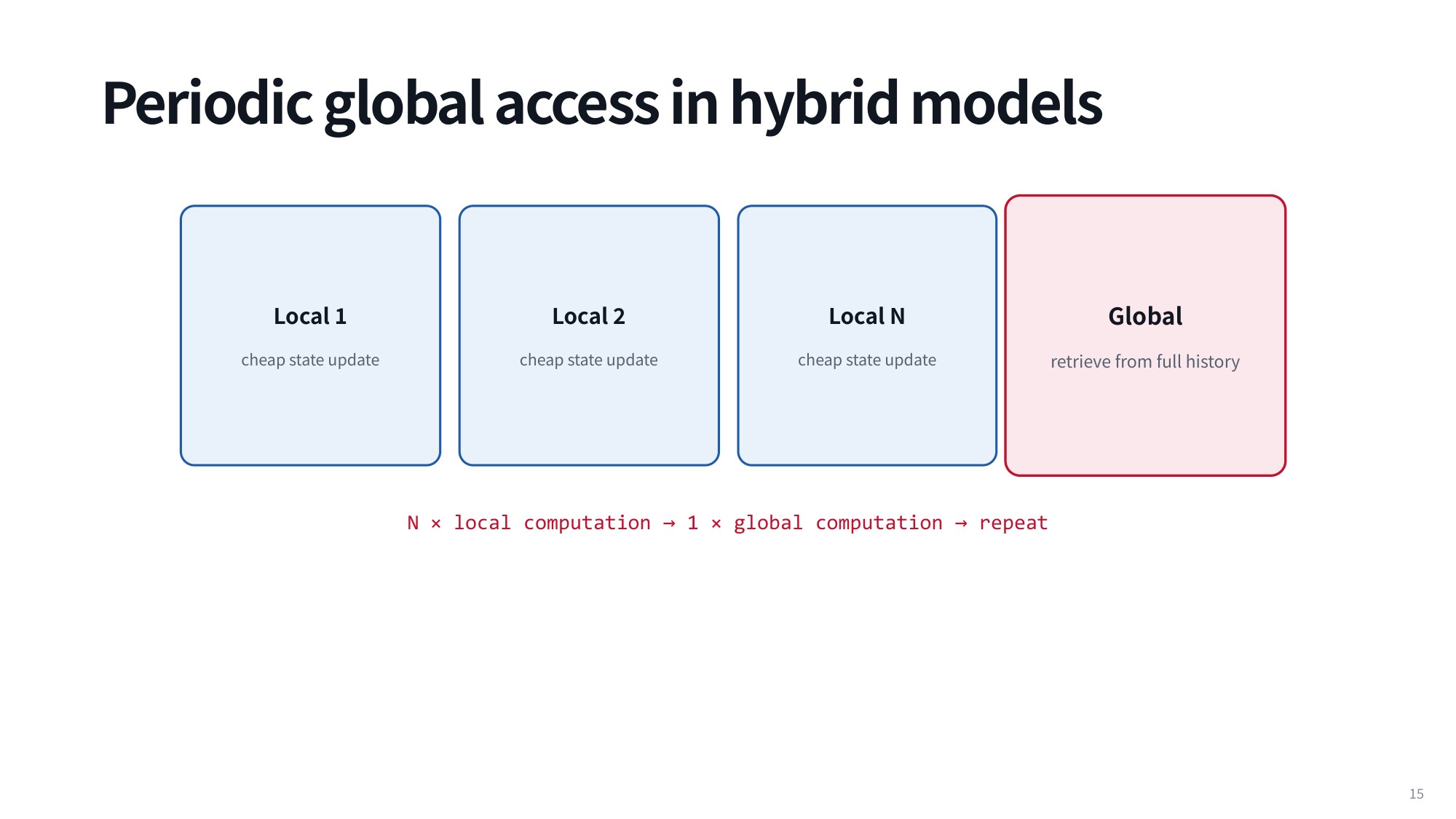
Fig 15. Periodic global access in hybrid models

Six frontier models show how consistent this pattern has become:

• Qwen3.8-Flash-Next uses Gated DeltaNet locally and QSA sparse retrieval globally, with 36 local layers to 12 global layers — roughly 3:1.
• GLM-5.3-Flash pairs Kimi Delta Attention locally with DSA + IndexPool globally, at 34:11, also roughly 3:1.
• Kimi K3 also uses Kimi Delta Attention locally, paired with dense Gated MLA globally, at 69:24 — again roughly 3:1.
• Nemotron 3 Ultra uses Mamba-2, a recurrent-style model, paired with dense GQA at 4:1.
• Inkling-Small pairs a 512-token sliding window with dense GQA at 5:1.
• DeepSeek-V4-Pro-0813 differs slightly, employing a 128-token window branch alongside compressed sparse/dense attention across interleaved branches.

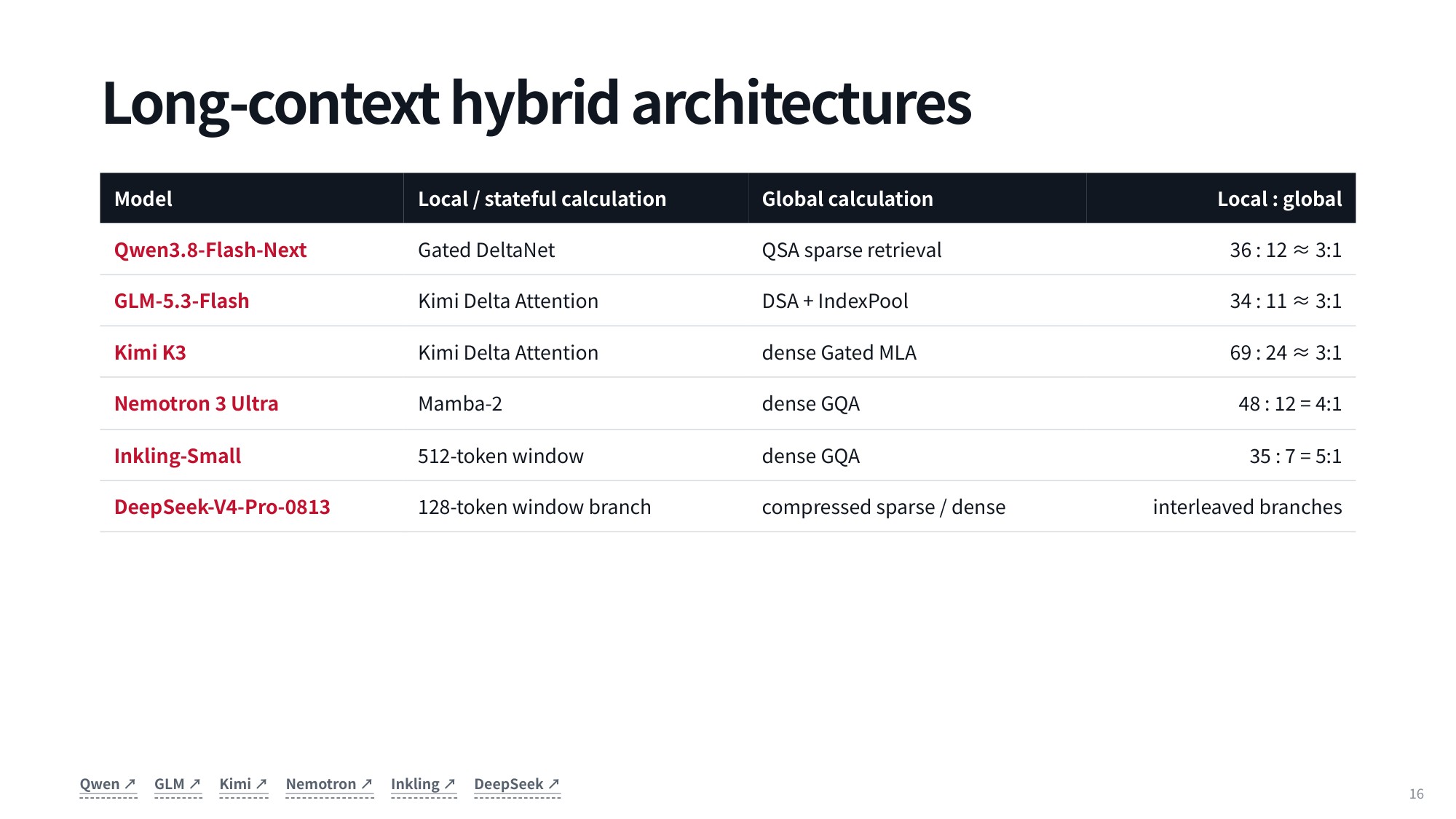
Fig 16. Long-context hybrid architectures

The industry standard, then, is a fast local mechanism combined with either sparse or dense global attention layers.

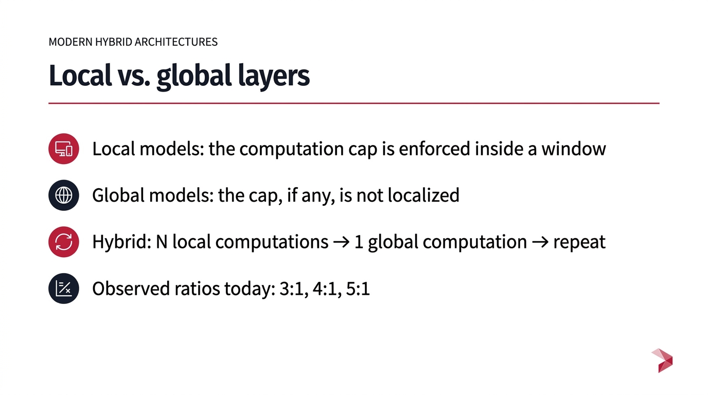
Fig 17. Local vs. global layers

9.3 Four Recurring Mechanisms

Why do these hybrids work? Look at the mechanisms they reuse. The simplest is sliding window attention.

Here the sequence is broken into chunks, and instead of attending back over the full sequence, the model attends only to the current chunk plus a fixed number of preceding ones. With a 512-token current chunk you might keep another 512 tokens and a further 512 from earlier chunks and attend across those. No change to the attention operation itself is required.

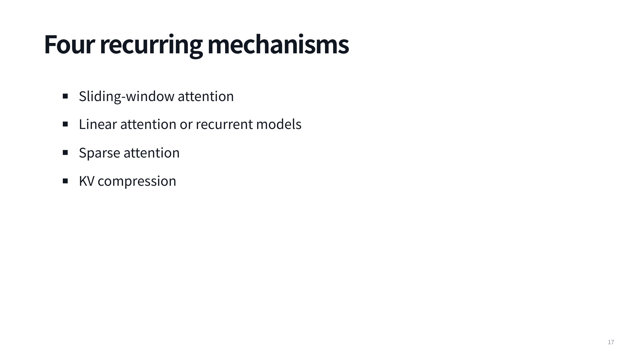
Fig 18. Four recurring mechanisms

The payoff shows up across layers. On the first layer, information reaches the current chunk only from the previous one or two chunks. By the next layer, those chunks have already absorbed information from their own predecessors. This hierarchical accumulation with depth gives you a gradually expanding context window, which is why sliding windows remain so widely adopted.

The more dominant route today, though, is some variety of linear attention. To see why, recall standard attention.

Standard attention relies on a (\text{softmax}) operation, and that operation is exactly what makes it expensive over long sequences: you take the exponent and normalize across all tokens. Because of the normalization, you must compute the full key-query multiplication matrix, which is quadratic.

Linear attention removes the (\text{softmax}) and its normalization from the formulation. The normalization matters less than you might expect, and once the (\text{softmax}) is gone, key-query multiplications become far cheaper. The cost is expressiveness: dropping the nonlinear transformation and normalization over the sequence makes linear attention definitively less expressive.

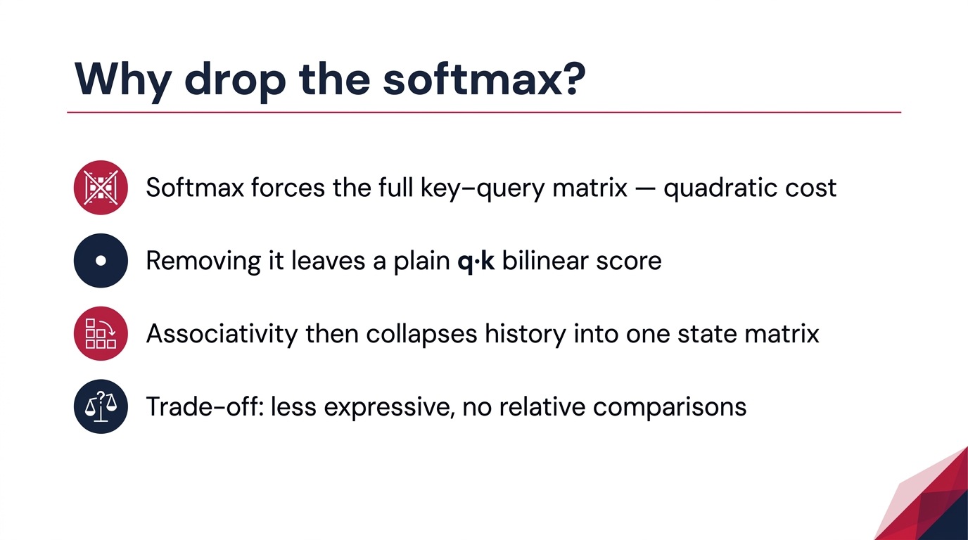
Fig 19. Why drop the softmax?

9.4 Production Implementations Across Frontier Models

Production models assemble these pieces in much the same way: local recurrent or windowed mechanisms combined with periodic global operations. The underlying mathematics gets involved, but the foundational concept behind each architecture is the same.

---

10. Sliding-Window Attention with Causal Window Masking

Full self-attention scales quadratically with sequence length, so at extremely long contexts the pairwise interactions between all tokens become intractable in both compute and memory. One straightforward fix is to restrict each token to a localized receptive field. This is sliding-window attention with causal window masking.

We introduce a parameter (w), the causal window size: the number of preceding positions each query keeps. Instead of reaching back to the start of the document, a query only sees the (w) most recent tokens before it.

[M_{ij}^{(w)} = \begin{cases} 0, & 0 \le i – j < w \ -\infty, & \text{otherwise} \end{cases}]

We enforce this by adding a causal window mask (M_{ij}^{(w)}) to the pre-softmax attention logits. For a query at index (i) and a key at index (j), we look at their relative distance: when (0 \le i – j < w), the key sits inside the active window, the mask contributes (0), and the raw dot-product score passes through untouched.

The other cases are blocked. If (j > i), the key lies in the future and must be hidden to preserve autoregressive causality. If (i – j \ge w), the key has fallen out of the retained local window. Both get (-\infty), which exponentiates to zero under the softmax and extinguishes those attention weights.

The attention formulation itself stays intact; only the band mask is new. That drops complexity from (O(n^2)) to (O(nw)) — linear in sequence length (n) for a fixed window (w).

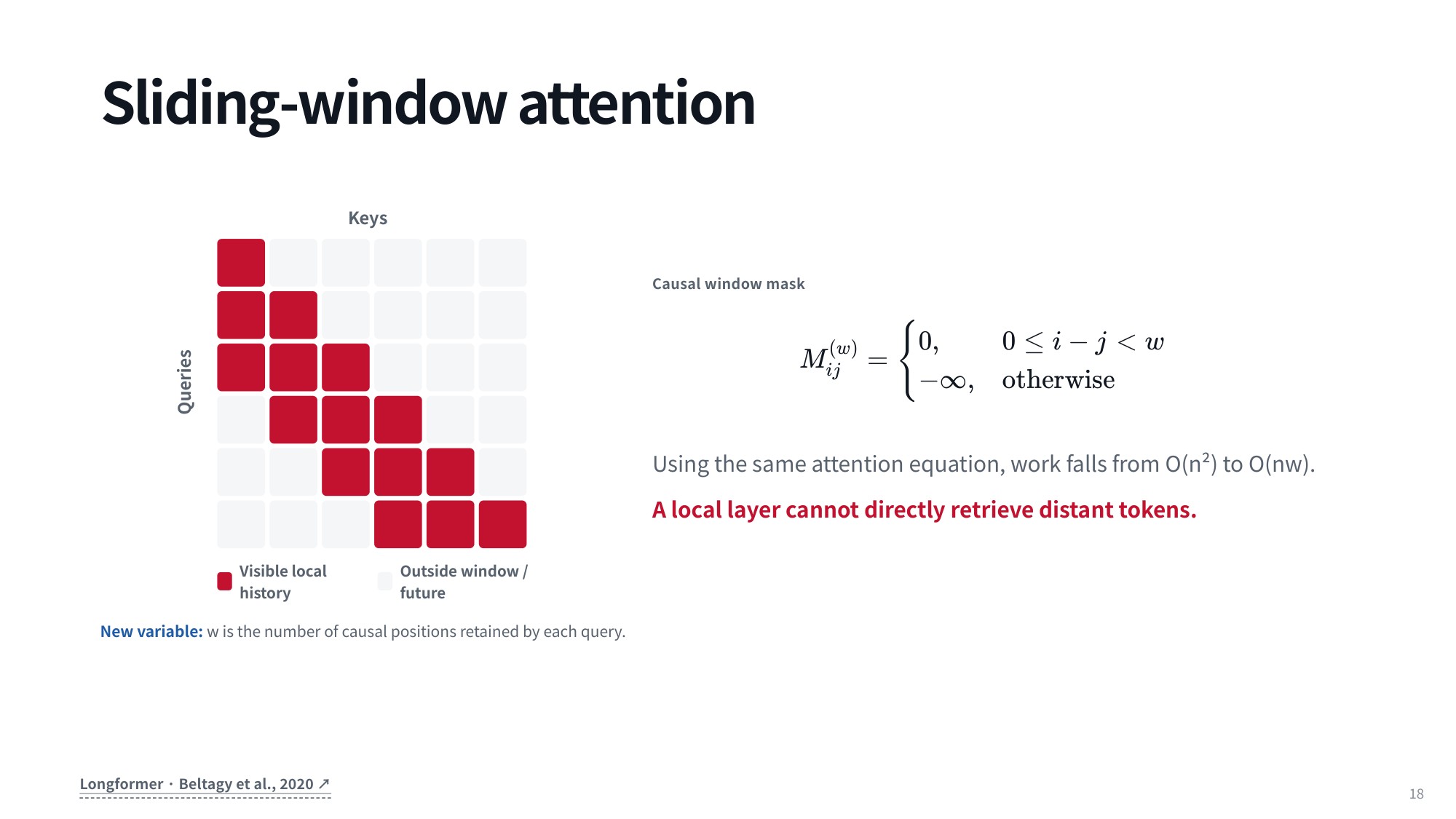
Fig 20. Sliding-window attention

The matrix view above makes the pattern concrete. Queries run vertically along the rows, keys horizontally across the columns, and the unmasked computations form a diagonal band of width (w).

Everything outside that stripe is zeroed. The upper triangle disappears because an autoregressive model cannot look ahead; the lower region beyond width (w) disappears because those tokens have aged out of the local window. This structural sparsity cuts both the active memory footprint and the arithmetic per generation step.

Local masking saves compute by discarding distant tokens. But what if we removed the softmax bottleneck altogether?

---

11. From Softmax to a Constant-Size Recurrent State

Sliding-window attention cuts computation by truncating the receptive field. A more radical option is to rewrite the attention operation itself. Modern efficient architectures follow a clear progression: standard softmax attention, then linear attention, then DeltaNet, then Gated DeltaNet, and finally designs like KDA (Kimi Delta Attention).

In causal softmax attention, the model scores a query against every preceding key and returns a weighted sum of the value vectors. The output (o_t) at step (t) comes from scaled query-key dot products, normalized by a softmax over all history positions (i \le t), multiplied by the values (v_i).

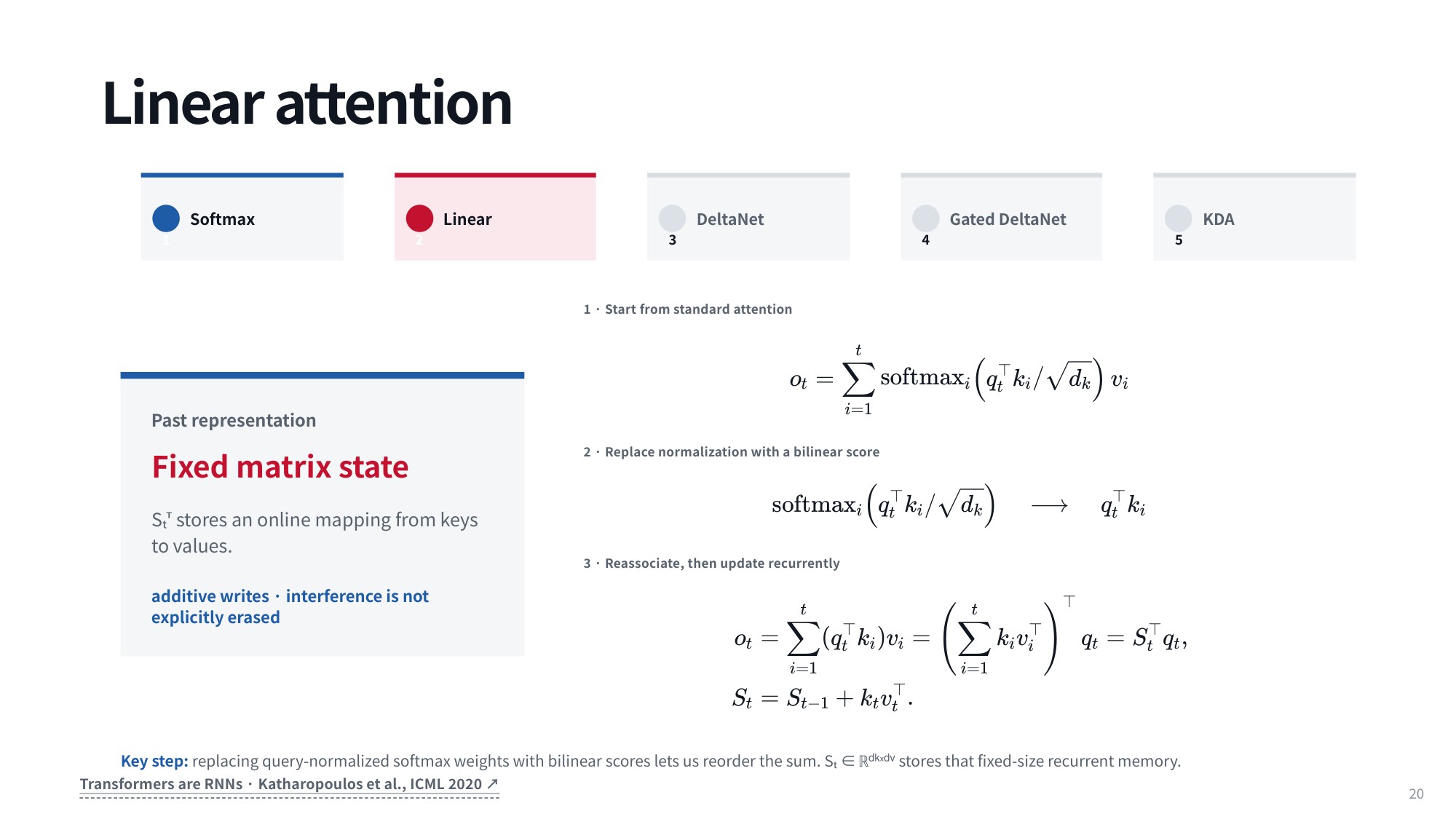
Fig 21. Linear attention

[o_t = \sum_{i=1}^t \mathrm{softmax}_i\left(q_t^\top k_i / \sqrt{d_k}\right) v_i]

The hurdle is that softmax couples each query with all previous keys at once. Its denominator sums over every past token, so you cannot factorize the computation or keep a compact running recurrence during autoregressive generation.

What happens if we drop the softmax entirely? The interaction between queries, keys and values collapses to an unnormalized inner product:

[\mathrm{softmax}_i\left(q_t^\top k_i / \sqrt{d_k}\right) \longrightarrow q_t^\top k_i]

Removing the non-linearity unlocks the associative property of matrix multiplication. Since (q_t^\top k_i) is a scalar, we can rearrange the terms and factor the query out of the summation over time steps instead of weighting each (v_i) separately.

[o_t = \sum_{i=1}^t (q_t^\top k_i) v_i = \left(\sum_{i=1}^t k_i v_i^\top\right)^\top q_t = S_t^\top q_t]

[S_t = S_{t-1} + k_t v_t^\top]

The summation over past keys and values isolates into an accumulated state matrix (S_t) — the sum of outer products between each key and its value, updated by a rank-one addition at every step. In this recurrent view, (S_t^\top) is an online associative memory: a linear function mapping a query straight to a value.

Standard attention is also a query-to-value map — take (q_t), attend over all keys, weight the values, output (o_t). The state matrix performs the same mapping through one compact representation. Instead of caching and re-reading every key and value across the context, as KV caching requires, the model keeps a single fixed-size memory state with the whole history compressed into it, and multiplies it by (q_t) when a new token arrives.

The state matrix updates incrementally in constant time, (\mathcal{O}(1)), per key-value pair via (S_t = S_{t-1} + k_t v_t^\top). The formulation is effectively a recurrent neural network: no full quadratic computation, and overall complexity drops from (\mathcal{O}(N^2)) to (\mathcal{O}(N)).

This dual representation bridges two worlds. During training, with all tokens known in advance, the operations run in parallel like standard attention. During autoregressive decoding you switch to the recurrent form, and because (S_t) has constant dimensionality regardless of sequence length, each token costs constant time and constant memory — no expanding KV cache blowing up GPU memory on million-token windows. That duality is the theoretical foundation for DeltaNet, Gated DeltaNet and KDA.

The trade-off is selectivity versus efficiency. Softmax turns arbitrary real numbers into probability-like weights between 0 and 1 that sum to 1, and that non-linearity lets the model focus sharply on a few previous tokens instead of spreading attention uniformly. Causal attention keeps every prior (k_i) and (v_i), comparing (q_t) against each one for crisp token-level access — at the price of (\mathcal{O}(t)) comparisons at every decoding step (t). Replacing the softmax with a plain bilinear score (q_t^\top k_i) removes the model’s ability to make relative comparisons across the sequence, and buys the associativity that collapses history into a constant-size state.

Compare this with the softmax stage on the progression bar, where (a_{t i}) is the normalized causal attention weight from query (t) to key (i):

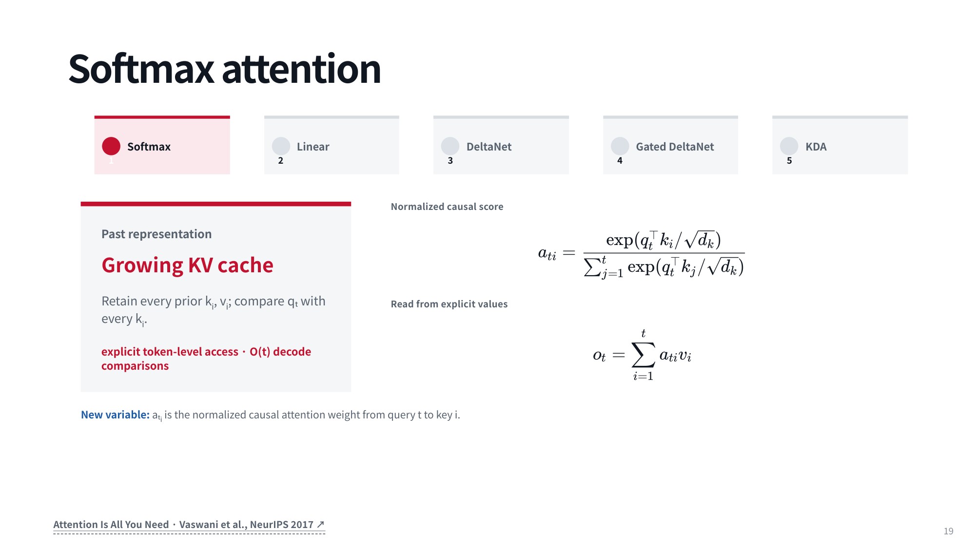
Fig 22. Softmax attention

[a_{t i}=\frac{\exp (q_t^{\top} k_i / \sqrt{d_k})}{\sum_{j=1}^t \exp (q_t^{\top} k_j / \sqrt{d_k})}]

[o_t=\sum_{i=1}^t a_{t i} v_i]

The denominator of (a_{t i}) couples all past keys (k_j) for (j \le t) through exponentiated dot products, so the terms cannot be reassociated. Softmax attention must retain every prior token representation and recompute the pairwise comparisons across the context window. Linear attention’s state (S_t) decouples query evaluation from history accumulation, giving constant-time inference updates.

The derivation in three steps:

• Drop the softmax. The normalized weight (\mathrm{softmax}_i(q_t^\top k_i / \sqrt{d_k})) becomes the plain bilinear score (q_t^\top k_i), costing us selective, relative comparisons across the sequence.
• Reassociate. Since (q_t^\top k_i) is a scalar, factor the query out of the summation and write (o_t = S_t^\top q_t).
• Keep a fixed-size state. History collapses into (S_t = S_{t-1} + k_t v_t^\top), updated in (\mathcal{O}(1)) per token, bringing total cost from (\mathcal{O}(N^2)) to (\mathcal{O}(N)) with constant memory at decode time.

---

12. Targeted Updates and Gated Retention in Recurrent Attention

12.1 DeltaNet: Memory Updates from Prediction Errors

Plain linear attention has one big caveat: standard linear recurrence is a less expressive function that cannot make relative comparisons between previous tokens. DeltaNet makes the formulation more expressive while keeping it attention-like, by predicting the value you want from the interaction of key (k_t) and the previous memory state (S_{t-1}).

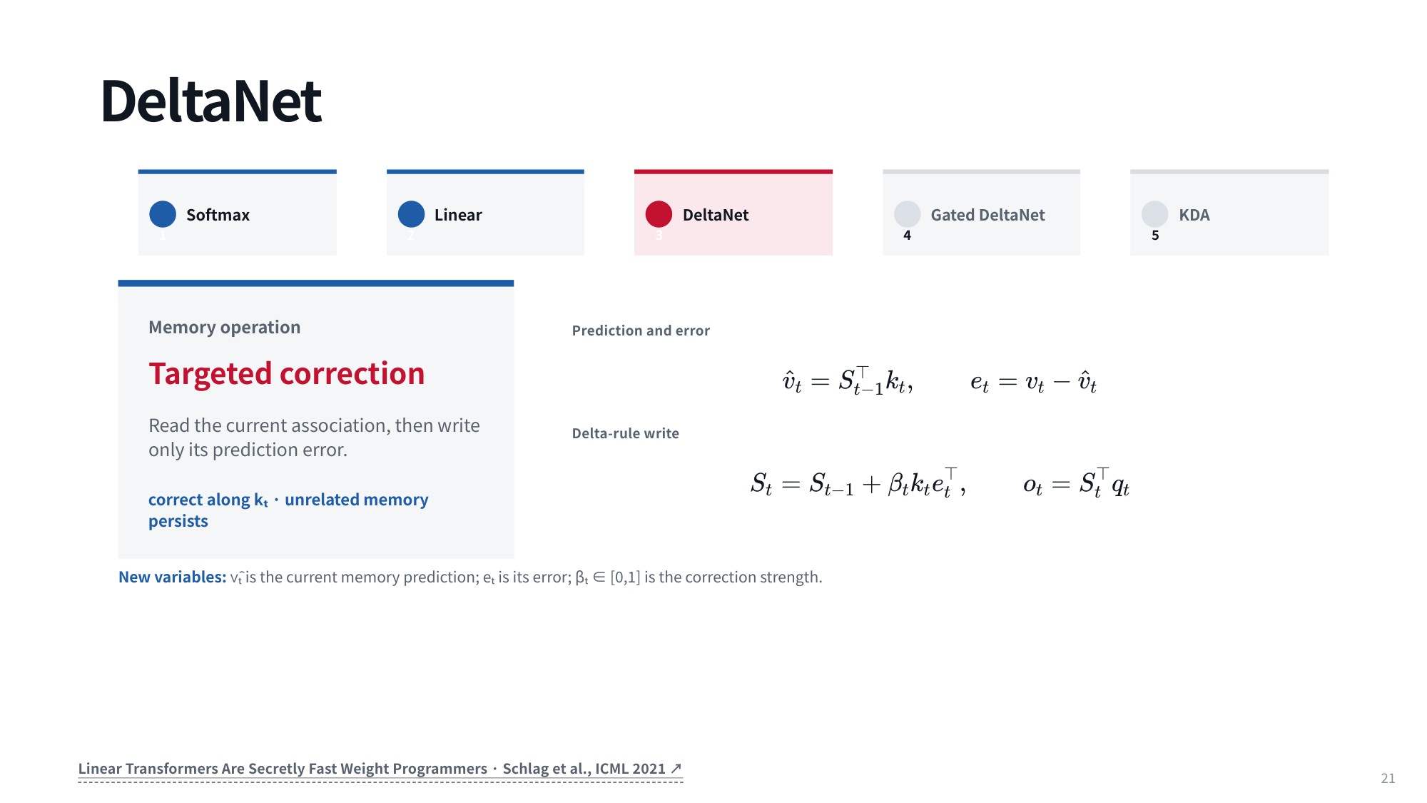
Fig 23. DeltaNet

The update introduces a few new variables: (\hat{v}_t) is the current memory prediction, (e_t) the resulting prediction error, and (\beta_t \in [0, 1]) controls how strongly the memory state is corrected.

[\hat{v}t = S{t-1}^\top k_t, \quad e_t = v_t – \hat{v}_t]

[S_t = S_{t-1} + \beta_t k_t e_t^\top, \quad o_t = S_t^\top q_t]

So you compute the predicted value (\hat{v}_t), compare it to the true value (v_t), form the error term (e_t), and add (k_t e_t^\top) scaled by (\beta_t). That step size acts like a learning rate, nudging the memory matrix toward the desired output without overshooting.

12.2 Gated DeltaNet: Scalar Retention Gates

Targeted error correction helps, but linear retention still has no way to stop distant context from adversely influencing future predictions.

Gated DeltaNet fixes this with an (\alpha_t) decay term that decays the memory matrix at every time step. Discounting past context dynamically lets you tune how local or non-local the retention is. Gated DeltaNet is used in the Qwen models, while Kimi and GLM push the idea further.

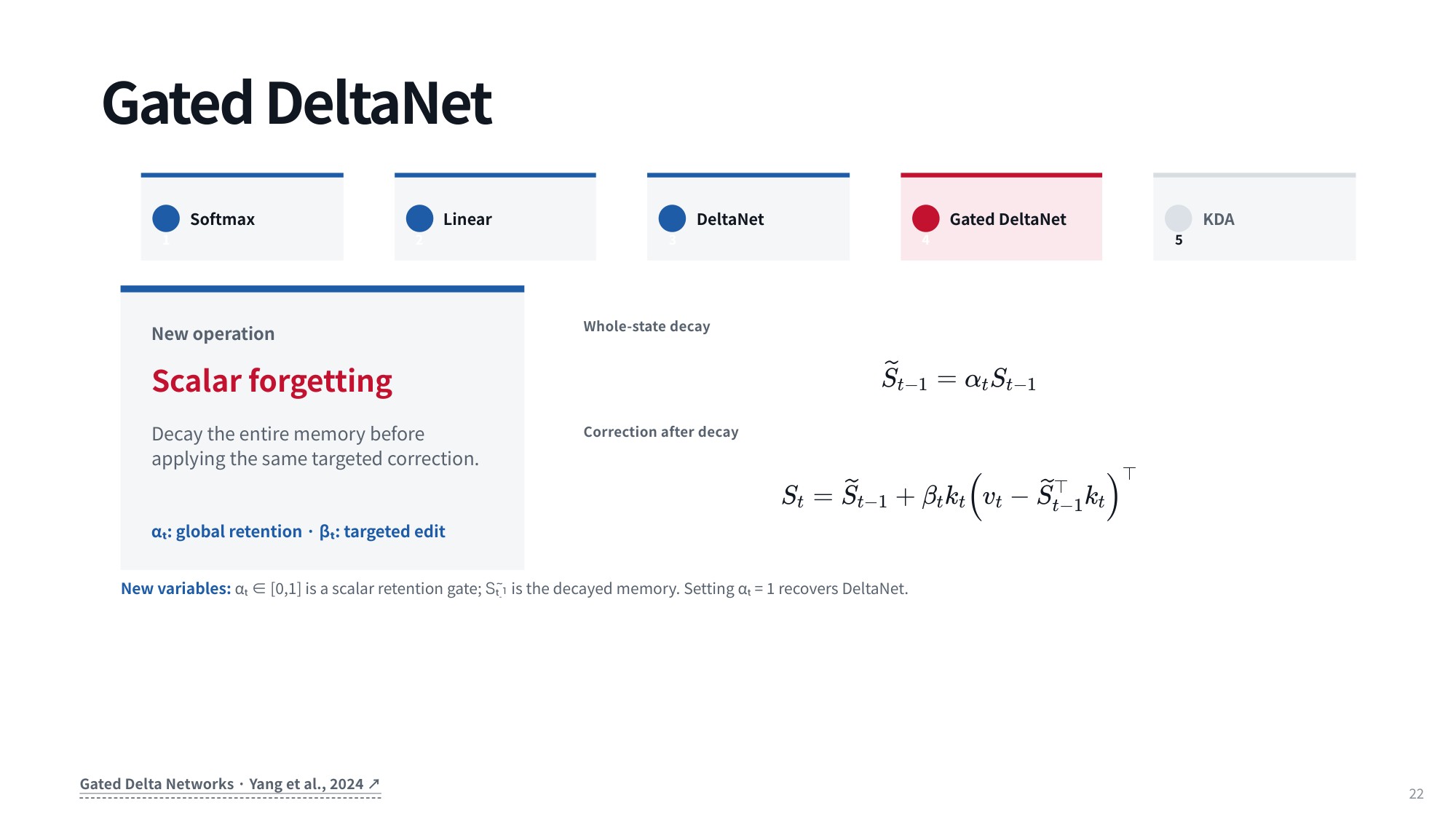
Fig 24. Gated DeltaNet

12.3 Kimi Delta Attention: Channelwise Gated Updates

GLM and Kimi use a per-element (channelwise) decay term, a slightly more expressive version of the same mechanism. Each element decays at its own speed, so parts of the context can survive over very long time spans while other parts fade almost immediately.

Kimi Delta Attention (KDA) is a way to turn the core idea of attention into something computable recurrently in context. The lecture traces the progression from Softmax attention to Linear attention, DeltaNet, and Gated DeltaNet; KDA is the step that adds channelwise gated recurrent updates.

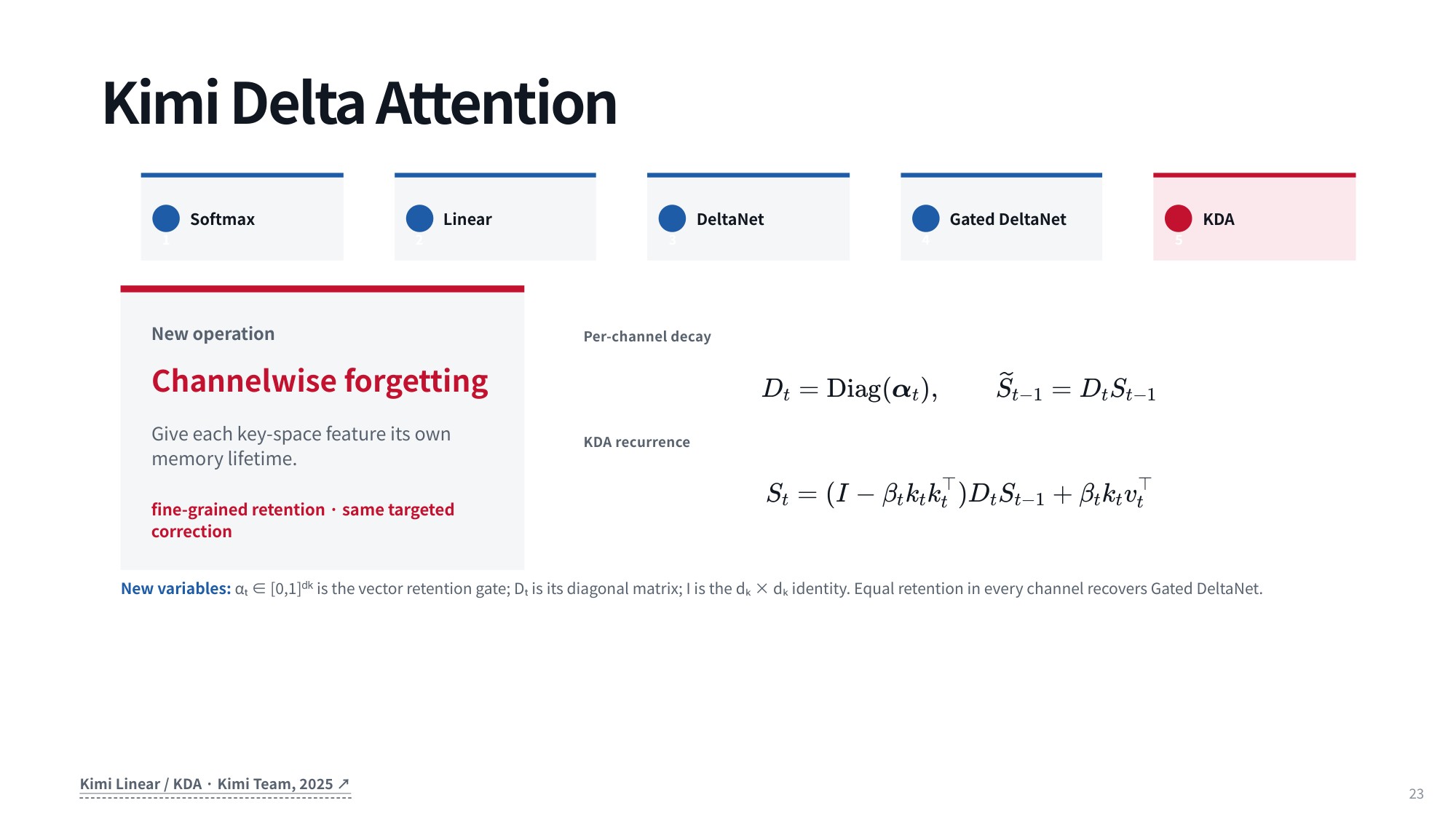
Fig 25. Kimi Delta Attention

Instead of a single uniform decay factor over the entire state, KDA defines a vector retention gate (\boldsymbol{\alpha}_t \in [0, 1]^{d_k}) and its corresponding diagonal matrix (D_t), so the model can selectively decay information across different feature channels.

[D_t = \operatorname{Diag}(\boldsymbol{\alpha}t), \quad \tilde{S}{t-1} = D_t S_{t-1}]

[S_t = (I – \beta_t k_t k_t^\top) D_t S_{t-1} + \beta_t k_t v_t^\top]

Here the gated previous state (\tilde{S}{t-1} = D_t S{t-1}) is modified by subtracting the projection onto key (k_t) scaled by (\beta_t), with (I) the (d_k \times d_k) identity matrix, and then adding the incoming association (\beta_t k_t v_t^\top).

Giving each channel an independent memory lifetime buys substantially more expressive flexibility for long-range dependencies. And if you set the retention equal in every channel, you recover Gated DeltaNet as a special case.

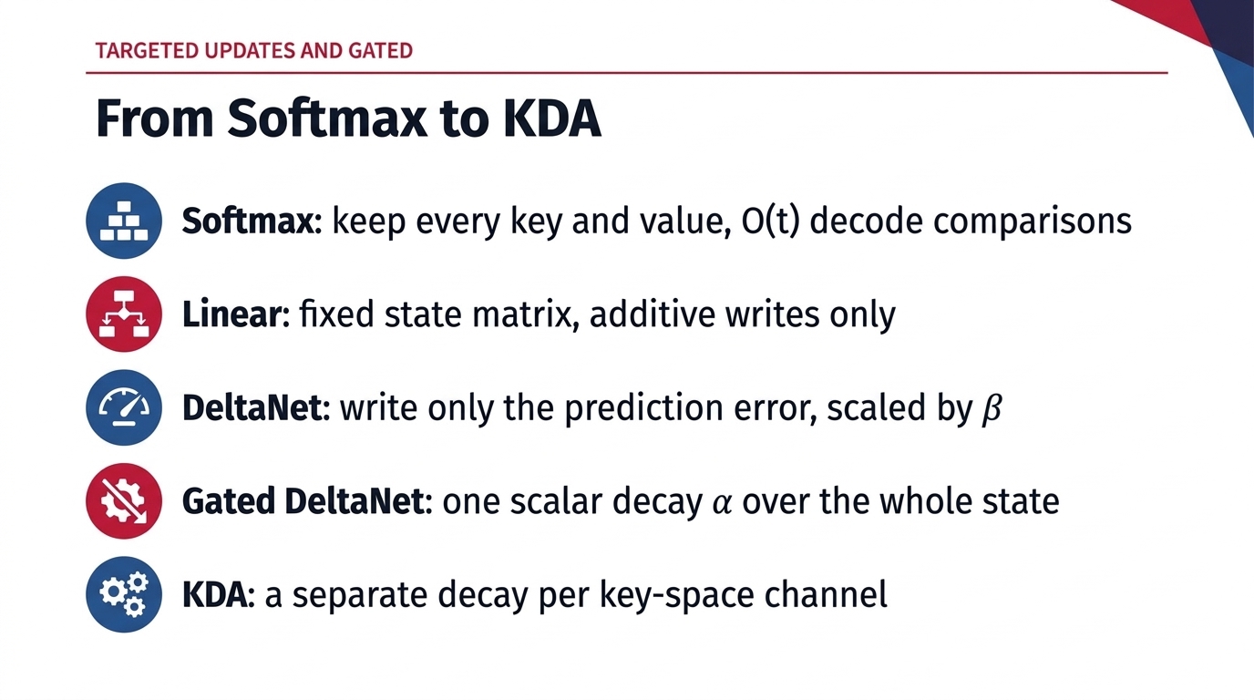
Fig 26. From Softmax to KDA

---

13. Sparse Attention: Fixed Topologies vs. Dynamic Content Routing

13.1 Restricting Attention to a Subset of Positions

Sparse attention means a query no longer looks at the entire previous context. Instead, it attends to a selected handful of tokens, which puts a hard limit on how many earlier positions are retrieved.

Formally, the computation is restricted to a subset of positions (S_i) instead of the full sequence. For each query vector (q_i), key vector (k_j), and value vector (v_j) with key dimensionality (d_k), the attention weights (A_{ij}) are normalized only across indices (j \in S_i), and the contextualized vector (o_i) is a weighted sum over that active subset:

[A_{ij} = \text{softmax}{j \in S_i} \left( \frac{q_i^\top k_j}{\sqrt{d_k}} \right), \quad o_i = \sum{j \in S_i} A_{ij} v_j]

How (S_i) is chosen is what separates the two families. A fixed topology (S_i^{\text{fixed}}) is completely input-independent, typically a local sliding window plus a fixed set of global positions (G). Dynamic, content-dependent routing instead uses a learned selector (g) to do query-specific top-(k) selection, producing a candidate set with fixed cardinality (|S_i^{\text{dyn}}| = K).

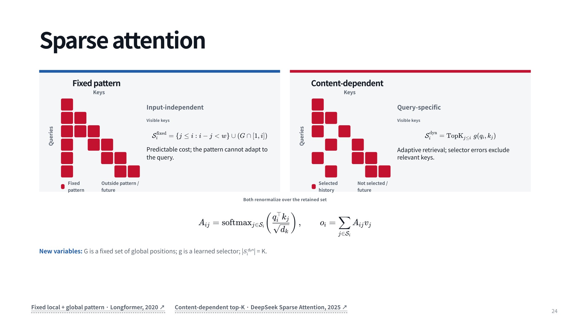
Fig 27. Sparse attention

13.2 Dynamic Top-K Selection

Fixed patterns give you rigid structure; dynamic selection keeps the same idea but makes the routing flexible.

The baseline is the fixed pattern, where attention goes to a fixed set of global positions (G) alongside local tokens. An early sparse attention paper from OpenAI (the Sparse Transformer), placed global attention roughly every 512 tokens. Because it samples at regular intervals, the complexity is still technically quadratic in sequence length — but it needs 512 times less computation than attending to every token, which is manageable enough over the contexts you care about.

The alternative is content-dependent sparse attention. Here you score candidates with a very cheap preliminary pass: down-project the attention vectors so they are extremely small, compute quick attention over those down-projected vectors with a learned selector (g), pick the top-(K) items to form (S_i^{\text{dyn}}) with (|S_i^{\text{dyn}}| = K), then run full attention only over those positions, using the same renormalized softmax as above. This is the routing strategy DeepSeek uses. The scoring metric is typically a plain dot product rather than cosine similarity, though the representations may be normalized beforehand — that implementation detail is not publicly confirmed.

The trade-off is straightforward. Fixed sparsity is very cheap, since you can write an optimized kernel that executes the pattern directly. Content-dependent sparsity needs two passes, one to select and one to attend, but it can be far more accurate. Both approaches are widely used in practice.

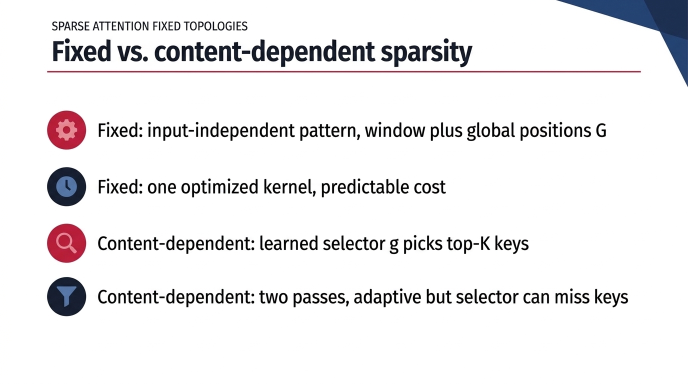
Fig 28. Fixed vs. content-dependent sparsity

---

14. KV Cache Compression: From MHA/MQA/GQA to Multi-Head Latent Attention

14.1 From MHA and MQA to GQA

Start with a baseline of (H) attention heads. Once sequences grow long, the KV cache becomes large and expensive, and it turns into the dominant bottleneck at serving time.

The standard fix in practice is grouped-query attention (GQA): use fewer heads than (H) — typically (H) divided by some power of two — but only for the keys and values.

Why does that help so much? The runtime cache stores keys and values, not queries (it is a KV cache, not a KVQ cache), so cutting the number of key and value heads cuts the memory footprint directly. Several query heads share one key/value head, which slashes cache overhead while keeping multi-head representations.

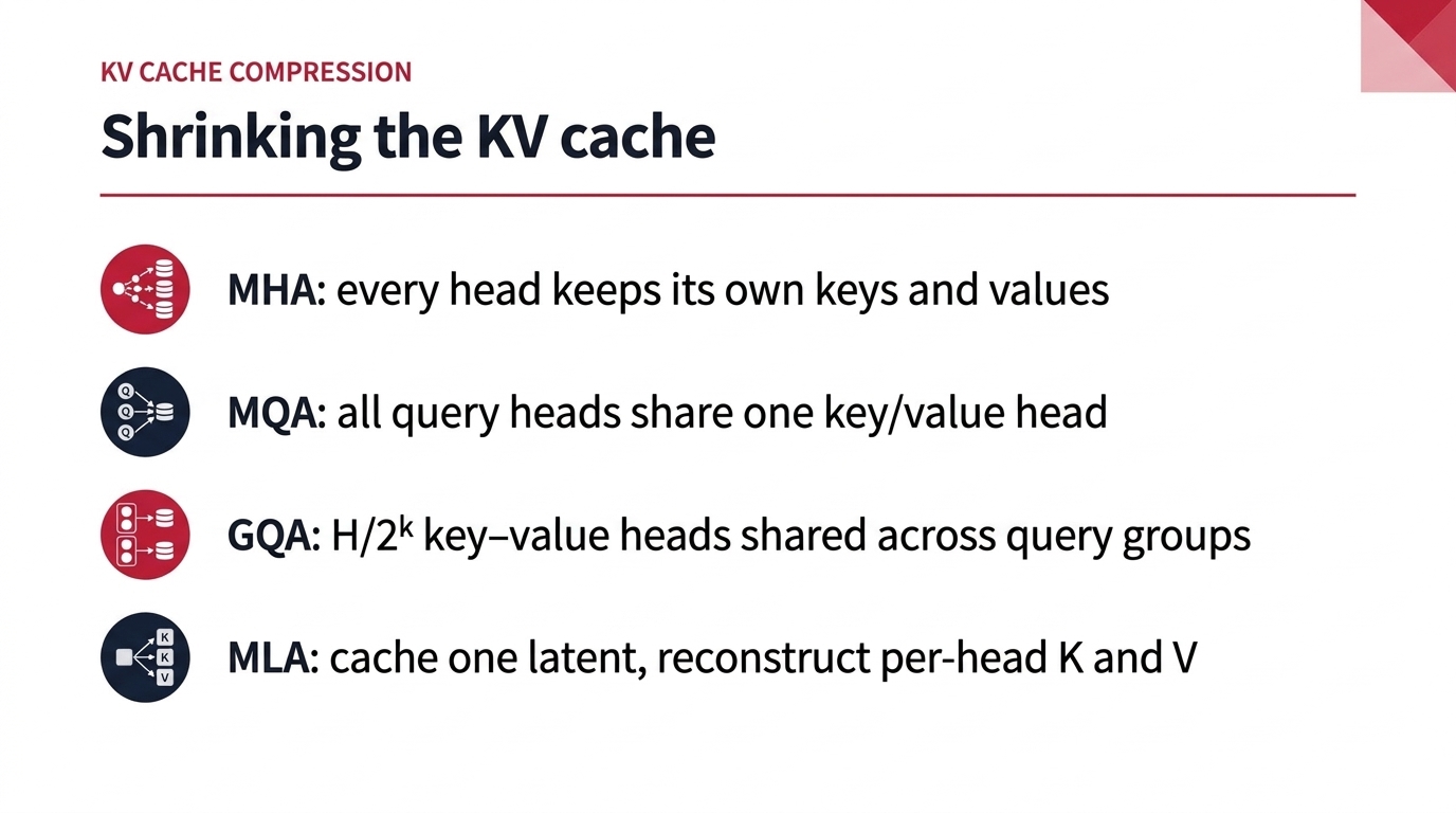
Fig 29. Shrinking the KV cache

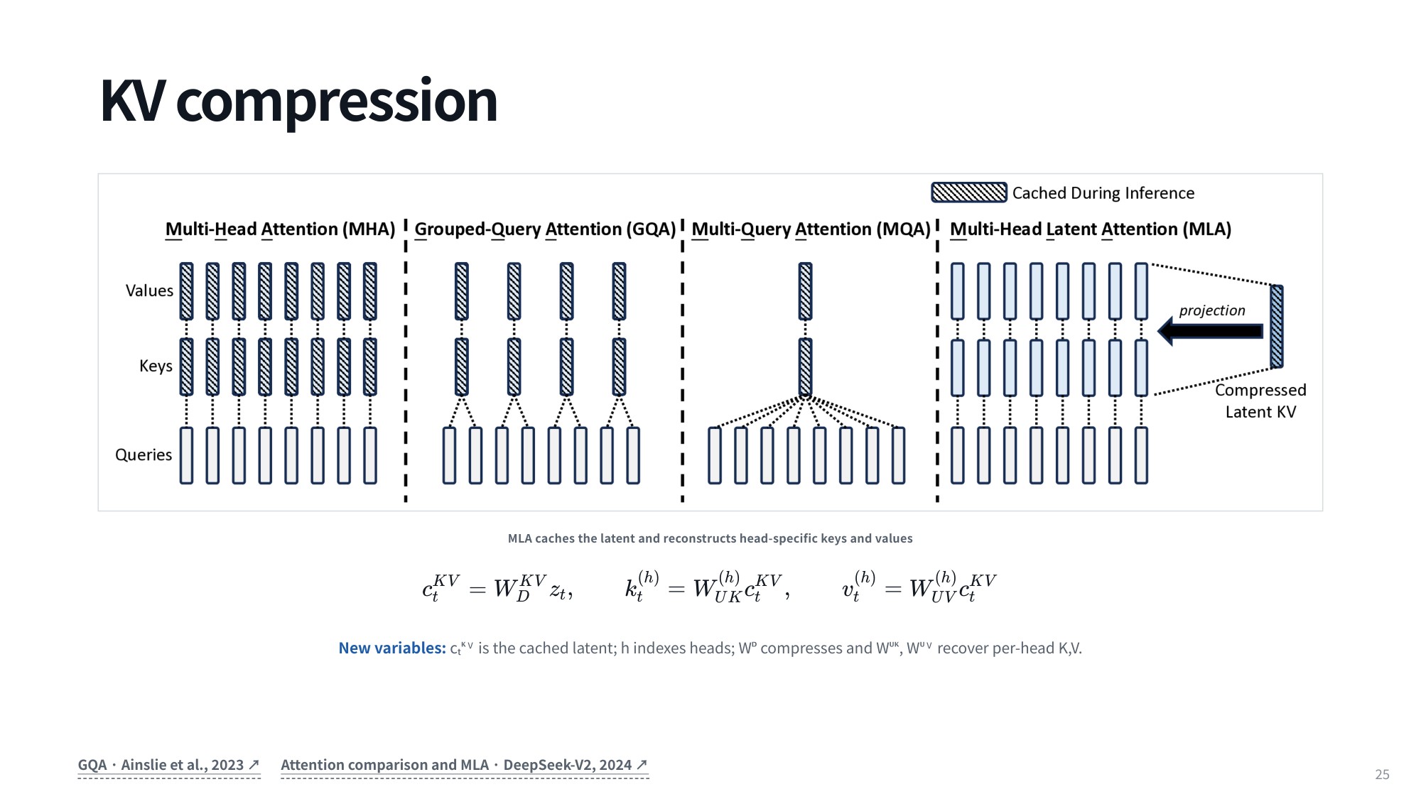
Fig 30. KV compression

There is a second strategy beyond reducing head counts: project keys and values into a shared low-rank latent instead of storing separate full-dimensional tensors per head. The formulation follows below.

14.2 Multi-Head Latent Attention (MLA)

Multi-Head Latent Attention (MLA) pushes that low-rank idea further. In standard multi-head attention every head keeps its own keys and values, each of dimension (D), multiplied across all heads — which scales memory quickly during generation.

MLA caches the latent and reconstructs head-specific keys and values:

[c_t^{KV} = W_D^{KV} z_t, \quad k_t^{(h)} = W_{UK}^{(h)} c_t^{KV}, \quad v_t^{(h)} = W_{UV}^{(h)} c_t^{KV}]

A down-projection matrix (W^D) (written as (W_D^{KV})) compresses the hidden state (z_t) into a single cached latent vector (c_t^{KV}) at time step (t). At attention time, the up-projection matrices (W^{UK}) and (W^{UV}) recover the per-head keys (k_t^{(h)}) and values (v_t^{(h)}) for head (h) from that cached latent. The result: high representational capacity with memory usage kept under control.

---

15. Summary

Four things are worth carrying away from this material.

1. Context growth is quadratic, not linear. An agent’s history grows linearly with the number of calls, but the total input you process grows quadratically: with a 1K system prompt and 5K tokens added per call, the per-call inputs are 6K, 11K, 16K, 21K, 26K, and the cumulative processed input is 6K, 17K, 33K, 54K, 80K after only five calls.
2. Long context hurts in two different places. Capacity is whether the model can actually use the tokens — needle-in-a-haystack style evaluations show this degrades long before the advertised limit. Efficiency is whether the system can afford to serve it, split between the compute-intensive prefill stage and the sequential, memory-bandwidth-bound decode stage.
3. The practical fixes cap the number of comparisons per step. Local windows turn (O(n^2)) into (O(wn)), linear and recurrent mechanisms (linear attention, DeltaNet, Gated DeltaNet, Kimi Delta Attention) turn it into (O(n)) with a fixed-size state, sparse attention keeps only a retained set per query, and KV compression (GQA, MLA) shrinks what you hold in memory. Almost every current frontier model is a hybrid: N local layers, then one global layer, repeated.
4. Measure what these choices actually move. Time to first token, time per output token, throughput and cost per request — plus how large your prompt really is and how much of it is system prompt, tool calls and tool results, so you know which mechanism is worth adopting.

Put together, the picture is coherent. Autonomous agent workflows scale their input prompts quadratically over sequential turns, and measurements on real coding agents such as OpenHands show that environment feedback, scaffolding and tool results dominate the conversation history, pushing context into tens of thousands of tokens within modest sessions. Dense causal self-attention becomes prohibitively expensive at that length, while retrieval benchmarks show the effective context window degrading well before the advertised limit, which surfaces as forgotten instructions and broken execution.

To balance capacity against serving efficiency across compute-bound prefill and memory-bound decode, frontier models have moved away from pure dense causal attention toward hybrid architectures. Interleaving fast local mechanisms — sliding-window masking, linear attention via associative reordering, DeltaNet error corrections, Kimi Delta Attention’s channelwise gating — with periodic global or sparse layers buys linear runtime while preserving cross-sequence expressivity.

On top of those backbones, serving infrastructure leans on KV cache compression to keep memory in check during autoregressive generation. GQA (grouped-query attention) and MLA (multi-head latent attention) compress key-value representations into low-rank latent spaces without giving up much representational fidelity. As multi-day agent sessions and millions of concurrent users become normal, these architectural and cache-management trade-offs are what will decide which autonomous systems actually scale.

---

Source

Lecture: Context Management for Long-Context Agents by Graham Neubig, Carnegie Mellon University.
Course: CMU 11-768 AI Agents (Fall 2026), Lecture 3, first half.
Video: YouTube. Slides: PDF. Course page: cmu-agents.com.

Further reading referenced in the lecture:

• DistServe (prefill/decode, TTFT/TPOT) — Zhong et al., OSDI 2024
• Needle-in-a-haystack evaluation — Kamradt, 2023
• Longformer — Beltagy et al., 2020
• Transformers are RNNs (linear attention) — Katharopoulos et al., ICML 2020
• Linear Transformers Are Secretly Fast Weight Programmers (DeltaNet) — Schlag et al., 2021
• Gated Delta Networks — Yang et al., 2024
• Kimi Linear / Kimi Delta Attention — Kimi Team, 2025
• DeepSeek Sparse Attention — 2025
• GQA — Ainslie et al., 2023; MLA — DeepSeek-V2, 2024

---

dataHacker.rs — LLM_log #030: Why Agent Context Explodes — Quadratic Growth, Serving Costs, and Efficient Attention (Linear, DeltaNet, KDA, MLA). By Vladimir Matic.