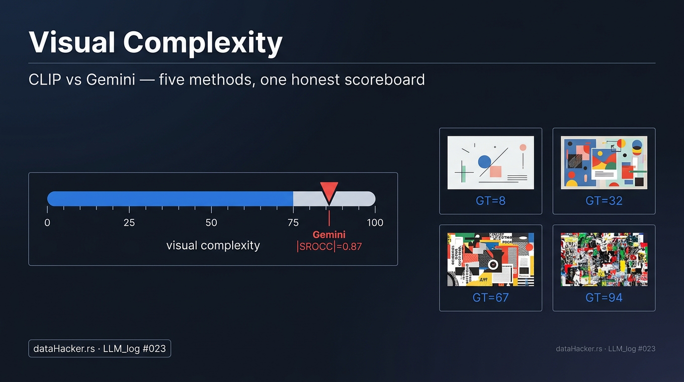
LLM_log #023: Visual Complexity Scoring — CLIP vs Gemini on SAVOIAS Advertisements
Highlights:
In this post we try to answer one practical question: can we score the visual complexity of an image without humans in the loop? We grab the SAVOIAS dataset (1,420 images with human-rated complexity), focus on the 200 advertisements, and try five different recipes — zero-shot CLIP prompts, Ridge regression on CLIP embeddings, pairwise ranking on embedding differences, kNN retrieval on cosine similarity, and finally Gemini 2.5 Pro as a chain-of-thought judge. The headline: every CLIP-based method collapses on truly held-out data once we strip the leakage, and only Gemini delivers a usable score. This includes the pairwise tournament estimator that looked promising at SROCC ≈ 0.84 in the deep-dive — that number was driven entirely by the classifier having seen the test items at train time. Retrain the classifier honestly on a 190/10 split and the tournament drops to SROCC ≈ 0.21 (exp7b, §13). Every number below is reproducible from a single Colab cell and ten cheap API calls. Let’s dig in.
Tutorial Overview:
- The Question — Why Score Complexity at All?
- SAVOIAS — How the Ground Truth Was Built
- The Frozen CLIP Backbone
- Method 1 — Zero-shot CLIP Prompts
- Method 2 — Ridge Regression on CLIP Embeddings
- Method 3 — Pairwise on Embedding Differences
- The Pairwise Pipeline in 10 Pictures
- Method 4 — kNN on CLIP Cosine Similarity
- Method 5 — Gemini-as-Judge with Chain of Thought
- Few-Shot Gemini — Does Calibration Help?
- The Honest Held-Out Scoreboard
- Why CLIP-Based Methods Fail (Semantic ≠ Complexity)
- The Honest Tournament Test, and Implications
- Summary
1. The Question — Why Score Complexity at All?
Visual complexity is the perceived busyness of an image — how many objects fight for the eye, how much text crowds the layout, how dense the patterns are. It matters in advertising (cluttered ads are forgotten), packaging design (busy labels lose at the shelf), UI (over-dense screens fatigue users), and image retrieval (a “minimalist scene” search needs a notion of simplicity).
The naive recipe is to ask humans. Crowdsource thousands of pairwise judgments — “which of A and B is more complex?” — fit Bradley-Terry, get one score per image on 0–100. That is exactly how the SAVOIAS dataset was built. But for production, paying humans for every new image is impractical. So the question becomes: can a frozen vision model do this for us?
Five recipes go on the bench in this post, all sharing the same 200 SAVOIAS advertisements. Spoiler: the simplest model wins.
2. SAVOIAS — How the Ground Truth Was Built
SAVOIAS holds 1,420 images across seven categories. We focus on the Advertisement category (200 images, 170 .jpg + 30 .png). The complexity scores were derived from 37,000+ pairwise comparisons by 1,600+ crowdworkers on Figure-Eight. Importantly, raters only compared images inside a category — an interior was never compared to an ad. Bradley-Terry was fit per-category and the resulting scores were rescaled to 0–100 separately for each category.
Important caveat: SAVOIAS scores are not comparable across categories. An advertisement with GT = 80 sits in the busiest 20% of ads; an interior with GT = 80 sits in the busiest 20% of interiors. Every result in this post is within-category.
The advertisement subset spans the full range: min 0, max 100, mean 52.5. Filenames are integer stems (0.jpg, 1.png …) and the GT file lists them all as .png — a small mismatch you have to join by stem, not by filename string. Here is the score distribution:
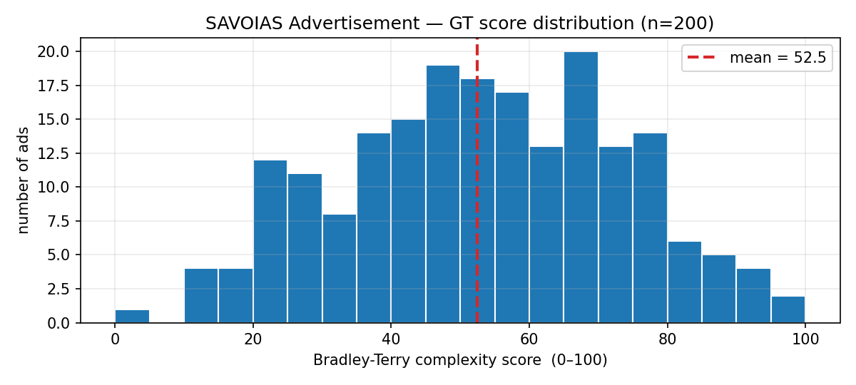
Fig 1. Histogram of the 200 Advertisement GT complexity scores. Mean 52.5, slight skew toward the complex end.
To get a feel for the scale, here is one median ad per decile:
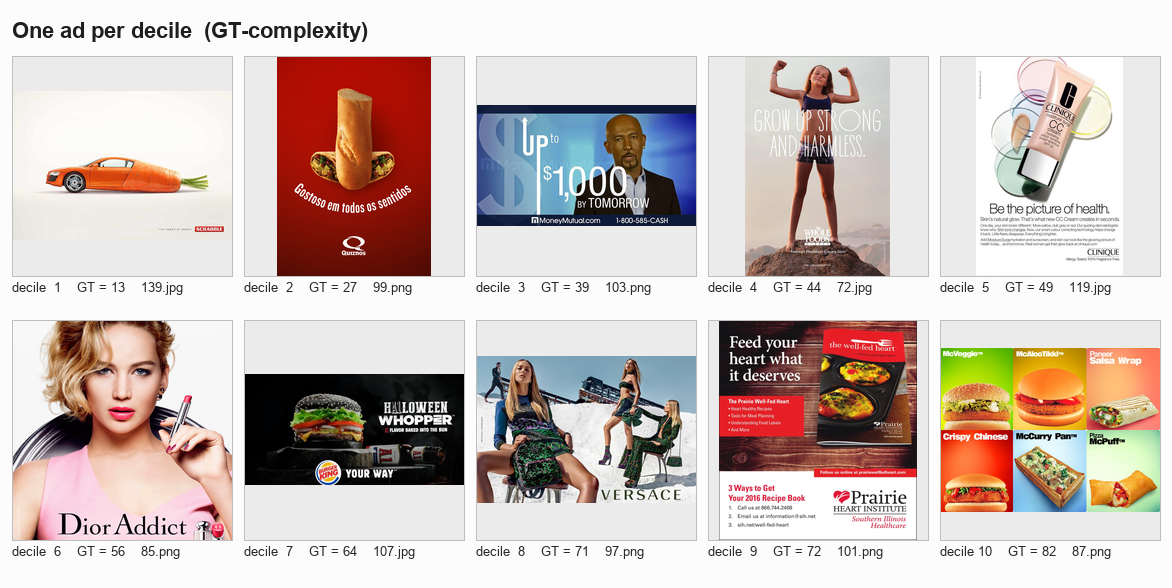
Fig 2. Decile sweep — one ad picked from each 10% slice of the GT distribution. Decile 1 = simplest 10%, decile 10 = busiest 10%.
3. The Frozen CLIP Backbone
Every classical method in this post sits on top of one shared frozen model: OpenAI CLIP ViT-L/14, loaded through open_clip_torch. We use only the image encoder. Total parameters \(\approx 304\) M, all frozen — no gradient ever flows in. Image preprocessing is the standard CLIP transform: resize the shorter side to 224, center-crop to \(224 \times 224\), normalize with CLIP’s own mean and std.
The visual transformer has 24 blocks, 16 heads, internal dimension 1024. After the final LayerNorm, the CLS token is projected from 1024 to 768 (the text-alignment projection trained on the contrastive objective). We L2-normalise the resulting 768-vector. Cached embeddings live in a single .npz on disk so all five methods read from the same cache:
import torch, open_clip
from PIL import Image

model, _, preprocess = open_clip.create_model_and_transforms(
    "ViT-L-14", pretrained="openai", device="cuda")
model.eval()
for p in model.parameters(): p.requires_grad_(False)

with torch.no_grad():
    img = preprocess(Image.open(path).convert("RGB")).unsqueeze(0).cuda()
    emb = model.encode_image(img)                 # [1, 768]
    emb = emb / emb.norm(dim=-1, keepdim=True)    # L2-normalise
One forward pass on a CPU is ~80 ms; on an M2 MPS device ~15 ms. The full 200-ad cache builds in under 30 seconds.
4. Method 1 — Zero-shot CLIP Prompts
The simplest recipe ignores GT scores entirely. Encode two text prompts, measure cosine similarity to each image, take the softmax probability of the “complex” class as the predicted complexity score.
PROMPTS = [
    "a minimalist, simple, uncluttered advertisement",
    "a cluttered, busy, complex advertisement with lots of text and graphics",
]

import torch
tokens = open_clip.tokenize(PROMPTS).cuda()
with torch.no_grad():
    txt = model.encode_text(tokens)
    txt = txt / txt.norm(dim=-1, keepdim=True)    # [2, 768]

# X is the cached [200, 768] image-embedding matrix, L2-normed
sims = X @ txt.T.cpu().numpy()                    # [200, 2]
probs = (sims * 100.0).softmax(axis=1)            # CLIP logit scale
zero_shot_score = probs[:, 1] * 100               # high = complex
On all 200 ads the zero-shot Spearman is \(|\rho| = 0.55\). On a held-out 10-ad subset (we’ll fix this subset for every method) it drops to \(|\rho| = 0.30\). The two prompts simply do not span the actual complexity axis, and CLIP gets fooled by ads with a single bold headline.
5. Method 2 — Ridge Regression on CLIP Embeddings
The next obvious thing: fit a linear regression that maps the 768-d embedding to the 0–100 GT score, with \(L_2\) regularisation.
from sklearn.preprocessing import StandardScaler
from sklearn.linear_model import Ridge

scaler = StandardScaler().fit(X_train)
ridge  = Ridge(alpha=1.0).fit(scaler.transform(X_train), y_train)
y_pred = ridge.predict(scaler.transform(X_test))
Watch the leakage. Fit on all 200 ads and evaluate on the same 200 ads (or 5-fold CV with thin folds), and you will see SROCC \(\approx 0.38\) on this category. The number looks fine until you do a clean 190-train / 10-held-out split: SROCC collapses to −0.19, slightly anti-correlated. The original 0.38 was the small-fold interpolation flattering the model. Do not trust regression numbers without a truly held-out test set.
Ridge on CLIP embeddings simply does not transfer. The complexity axis is not expressible as a single linear weight over the 768 CLIP dimensions.
6. Method 3 — Pairwise on Embedding Differences
The trick learning-to-rank uses: instead of predicting a scalar, train a binary classifier on pairs. For pair \((i, j)\) the feature is \(\mathbf{x}_i – \mathbf{x}_j\) and the label is 1 if image \(i\) is more complex than \(j\). The trained weight vector \(\mathbf{w}\) is itself a scoring function: \(\text{score}(\mathbf{x}) = \mathbf{w} \cdot \mathbf{x}\). This is essentially RankNet without the depth.
from sklearn.linear_model import LogisticRegression
import numpy as np

rng = np.random.default_rng(42)
pairs = []
while len(pairs) < 6000:
    i, j = rng.integers(0, len(y_train), size=2)
    if i == j or abs(y_train[i] - y_train[j]) < 4.0:
        continue
    pairs.append((int(i), int(j), int(y_train[i] > y_train[j])))
pairs = np.array(pairs)
pos = pairs[pairs[:, 2] == 1][:1500]
neg = pairs[pairs[:, 2] == 0][:1500]
pairs = np.concatenate([pos, neg])

F = X_train[pairs[:, 0]] - X_train[pairs[:, 1]]
L = pairs[:, 2]
clf = LogisticRegression(fit_intercept=False, C=0.1, max_iter=2000).fit(F, L)

w        = clf.coef_[0]
y_score  = X_test @ w                     # global complexity score
When trained on pairs sampled from all 200 ads and then evaluated on the same 10 ads, this method scores SROCC = 0.78. The number looks great. It is wrong, for the same reason Ridge looked great in the deep dive: the 10 test ads appeared inside the 3,000 training pairs. Retrain the classifier on pairs drawn only from the 190 non-test ads and evaluate on the 10:
The honest pairwise number on truly held-out ads: SROCC \(\approx 0.18\), held-out pair accuracy \(\approx 56.5\%\) — barely above chance. The same leakage that flattered Ridge was flattering pairwise too. The natural follow-up — “what if we use the same classifier as a tournament discriminator against K labelled anchors, instead of as a pointwise regressor?” — is the architecture walked through in §7. The honest experiment is in §13: it doesn’t rescue the signal. Once the classifier is retrained on the 190 non-test ads, the tournament collapses to SROCC \(\approx 0.21\) as well. CLIP-difference, on this category, simply does not separate complexity.
7. The Pairwise Pipeline in 10 Pictures
Before we add the last two baselines, here is a visual walkthrough of what the pairwise tournament actually does end-to-end. The point is to make the data flow concrete — what is GT, what is the classifier output, what is the final prediction. Same colour key on every figure: blue = data from the labelled GT reference pool, orange = output of the trained pairwise classifier, red = the final predicted score, grey = audit-only.
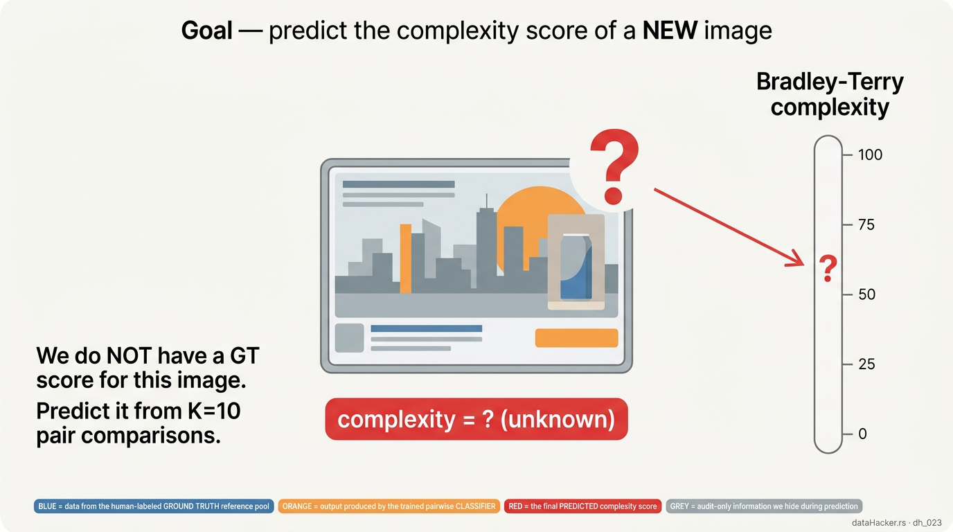
Fig 3. Setup. We have a new ad. We do NOT have its GT score. We want to predict it on the 0–100 scale from a handful of pair comparisons.
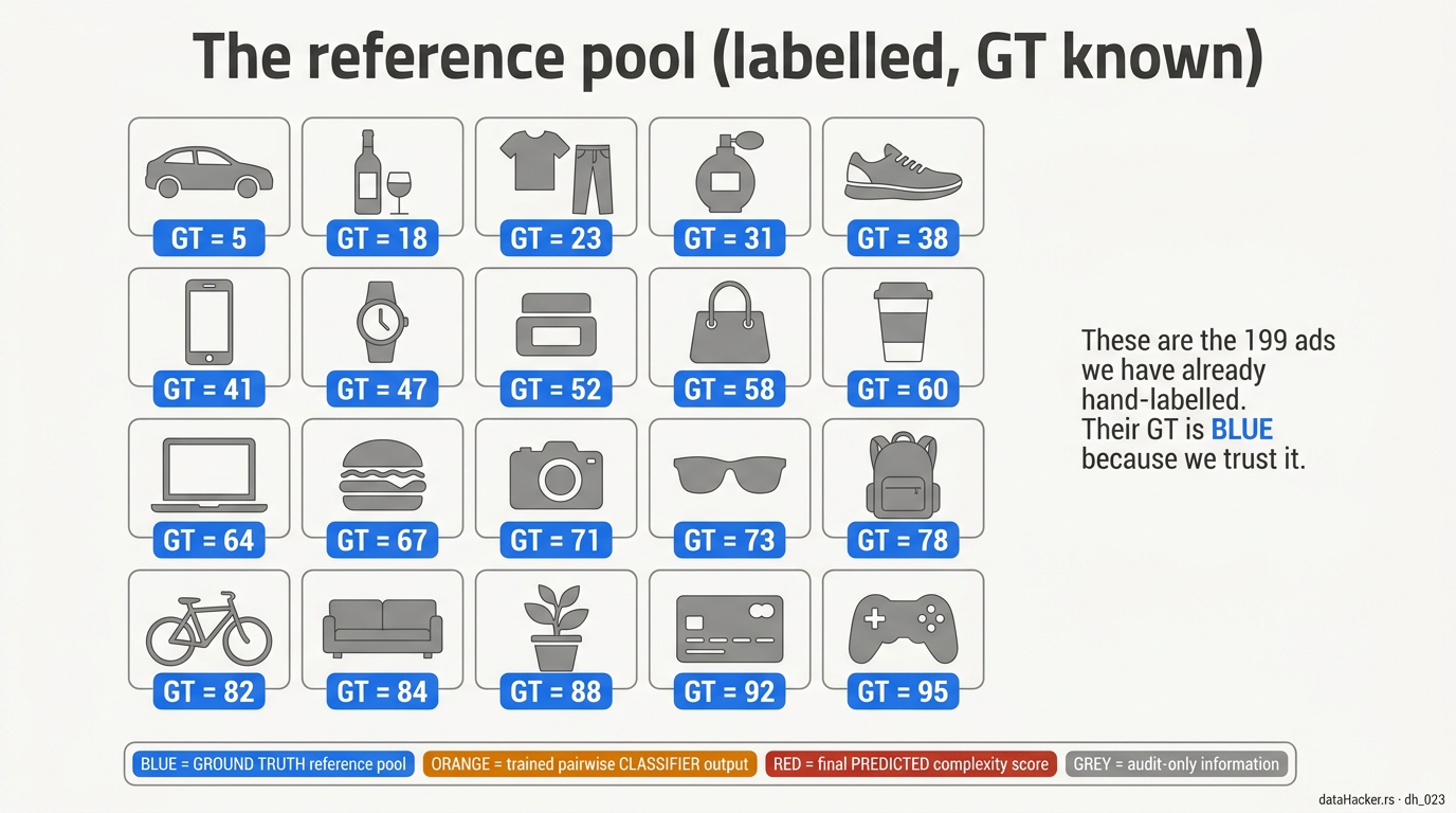
Fig 4. The reference pool. 199 ads we have already hand-labelled. Their GT is shown in blue because we trust it — these labels are what calibrate the rest of the pipeline.
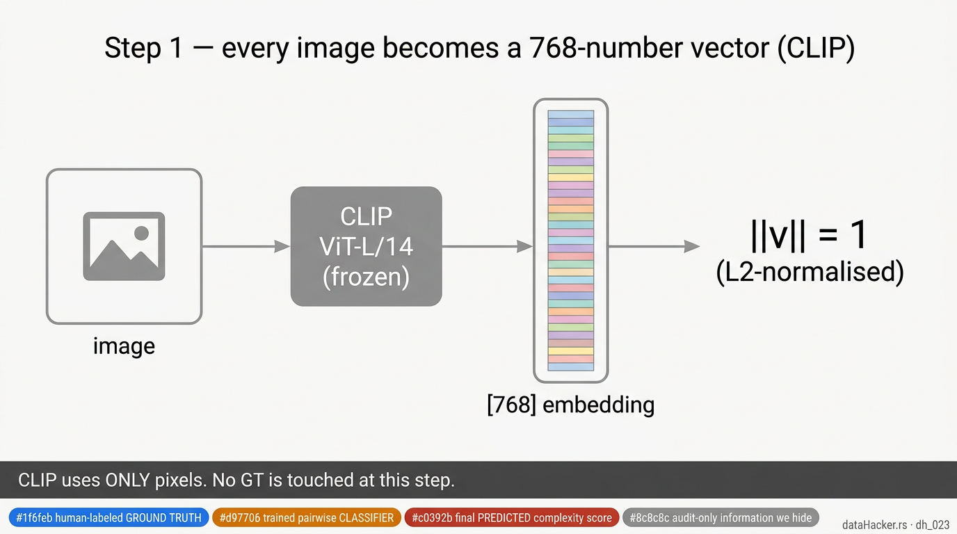
Fig 5. CLIP step. Every image — test or reference — goes through the same frozen CLIP ViT-L/14 to become a 768-dim vector. CLIP reads pixels only; no GT is touched in this step.
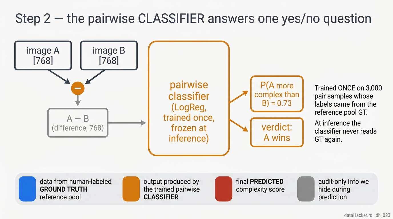
Fig 6. The pairwise classifier. Takes two image embeddings A and B, computes A − B, outputs the probability that A is more complex than B. Trained once on GT-labelled pairs; frozen at inference. The orange parts are the classifier’s output.
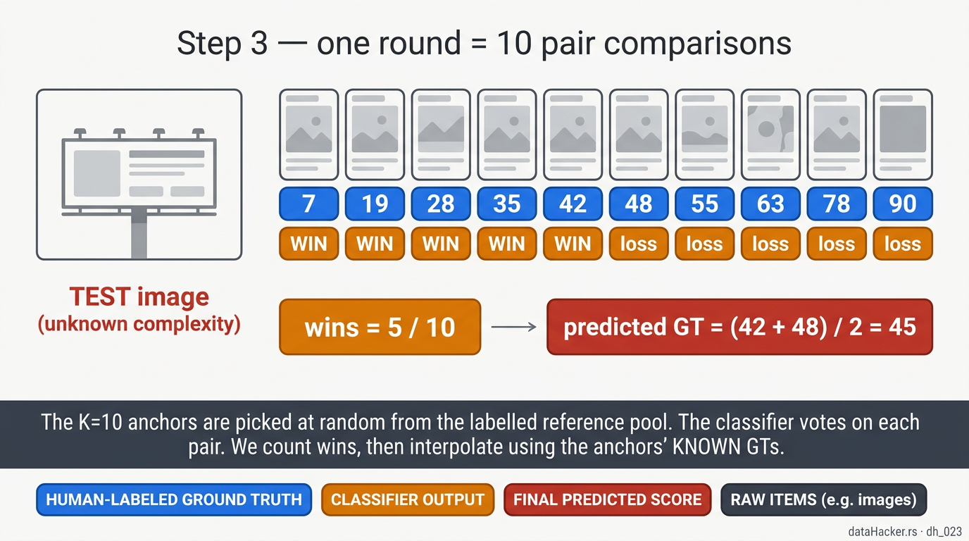
Fig 7. One tournament round. Sample K = 10 random anchors from the reference pool. Run the pairwise classifier 10 times — once per anchor. Five wins, five losses in this example.
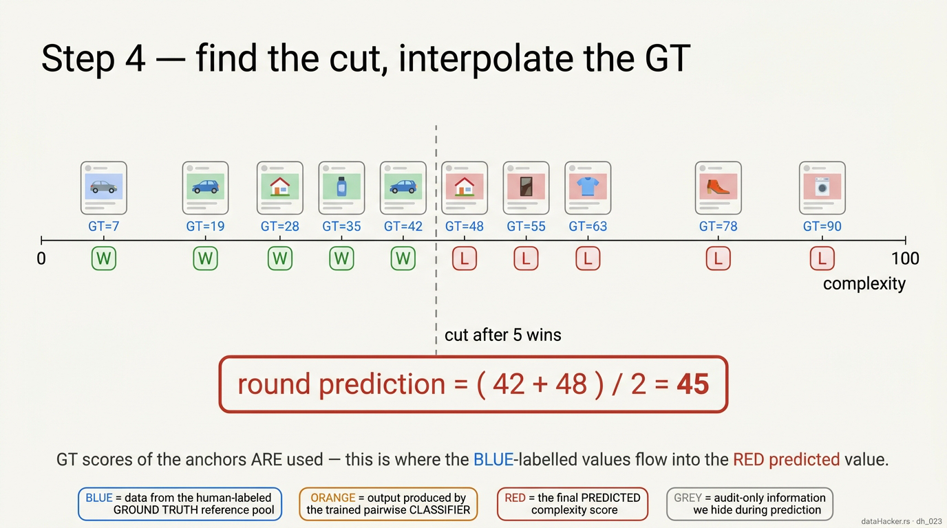
Fig 8. Sort and interpolate. Order the 10 anchors by their known GT. The test ad “fits between” the 5th and 6th anchor (5 wins, 5 losses). Predicted GT = midpoint = (42 + 48) / 2 = 45.
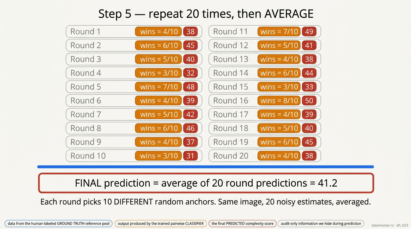
Fig 9. Twenty rounds. Each round picks 10 DIFFERENT random anchors. Average the 20 round predictions to wash out the classifier’s per-pair noise. Final prediction = the mean.
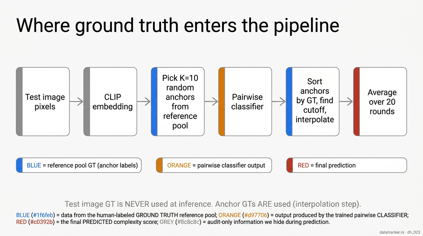
Fig 10. Where ground truth enters. The test image’s GT is NEVER used at inference. Anchor GTs ARE used — but only at the interpolation step, after the classifier has cast its votes.
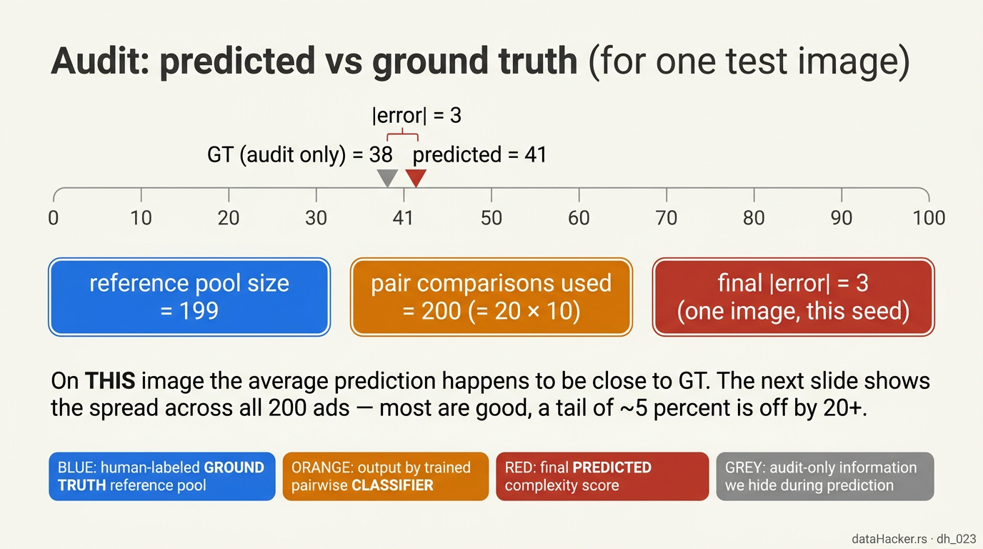
Fig 11. Audit on one image. After the prediction is locked in, we compare against the held-out GT to score the system. The GT was hidden the whole time; this step is just for evaluation.
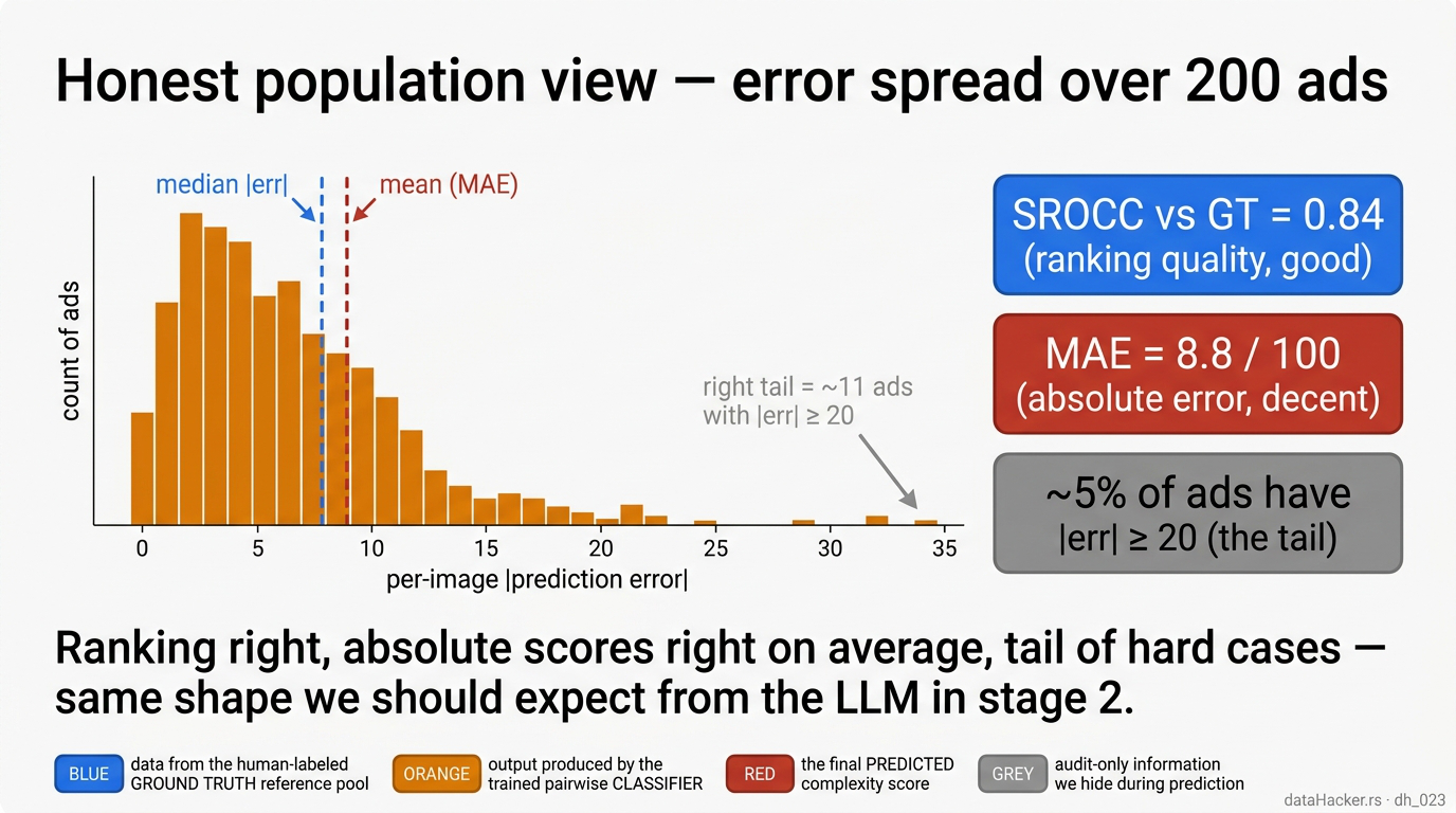
Fig 12. Population view of the tournament estimator in its original (leaky) form. Across the 200 ads, |error| has a long right tail — about 5% of ads have |err| ≥ 20. The tournament’s ranking looks right (SROCC ≈ 0.84, MAE 8.84 at K=20). Important caveat: the classifier here was trained on pairs sampled from all 200 ads, so the 10 test ads appeared in the classifier’s training pairs. §13 reruns this exact tournament with the classifier honestly retrained on 190 non-test ads only — SROCC collapses to 0.21 and MAE rises to 23. The 0.84 was 100% the classifier having seen the test items at train time.
Why this walkthrough still matters even though the architecture failed on this dataset. The pipeline above is the architecture the original LLM-pairwise plan was built around, and it is still the right shape for problems where (a) a strong pairwise discriminator exists, and (b) you cannot ship the image to a hosted LLM. What §13 shows is that on SAVOIAS Advertisement, condition (a) is not met — CLIP differences do not carry a usable complexity signal once leakage is removed, so the tournament has nothing to amplify. On a different backbone, or a category where complexity tracks something CLIP actually encodes (e.g. Interior Design at SROCC 0.79), the same architecture is still worth trying.
8. Method 4 — kNN on CLIP Cosine Similarity
If neither regression nor a linear ranker work, what about the laziest method of all? For each test ad, find the \(K\) closest training ads in CLIP cosine, take the mean of their GT scores. No model, no training step beyond CLIP itself.
import numpy as np

# X_train: [190, 768] L2-normed   y_train: [190]   x_test: [768]
sims = X_train @ x_test                # cosine similarity for unit-norm
order = np.argsort(-sims)[:7]          # top-7 neighbours
y_pred = float(np.mean(y_train[order]))
Result on the same 10 held-out ads: kNN-7 hits MAE \(\approx 18.7\), SROCC \(\approx 0.32\). Better than Ridge or honest pairwise, but still far below useful. A K-sweep from 1 to 190 confirms the verdict — no K rescues this method:
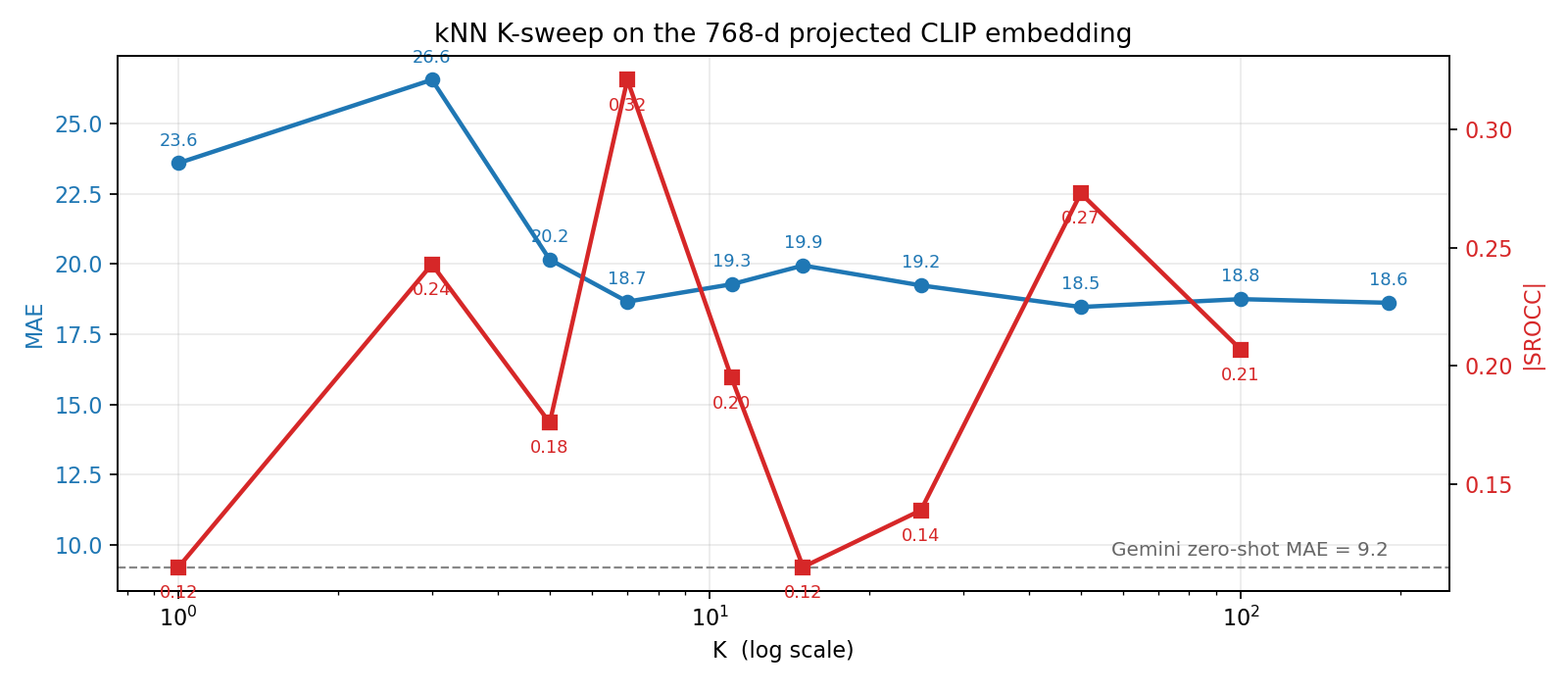
Fig 13. K-sweep from 1 to 190 on the projected 768-d CLIP feature. MAE is flat at \(\approx 19\) for any reasonable K. Dashed line = Gemini zero-shot MAE for reference.
We also tried the pre-projection 1024-d CLS hidden state (the feature CLIP produces before the 1024→768 text-alignment projection). It is marginally worse (MAE 19.2, SROCC 0.22) — the complexity signal is not hiding behind the projection, it is simply not there.
The failure mode is visually obvious. For one test ad with GT = 15 (minimalist sky), CLIP’s 7 nearest neighbours have GT scores of 13, 20, 39, 44, 49, 63, 67 — spread of 54 points. CLIP grouped them by subject matter (people on light backgrounds, clean compositions), not by complexity:
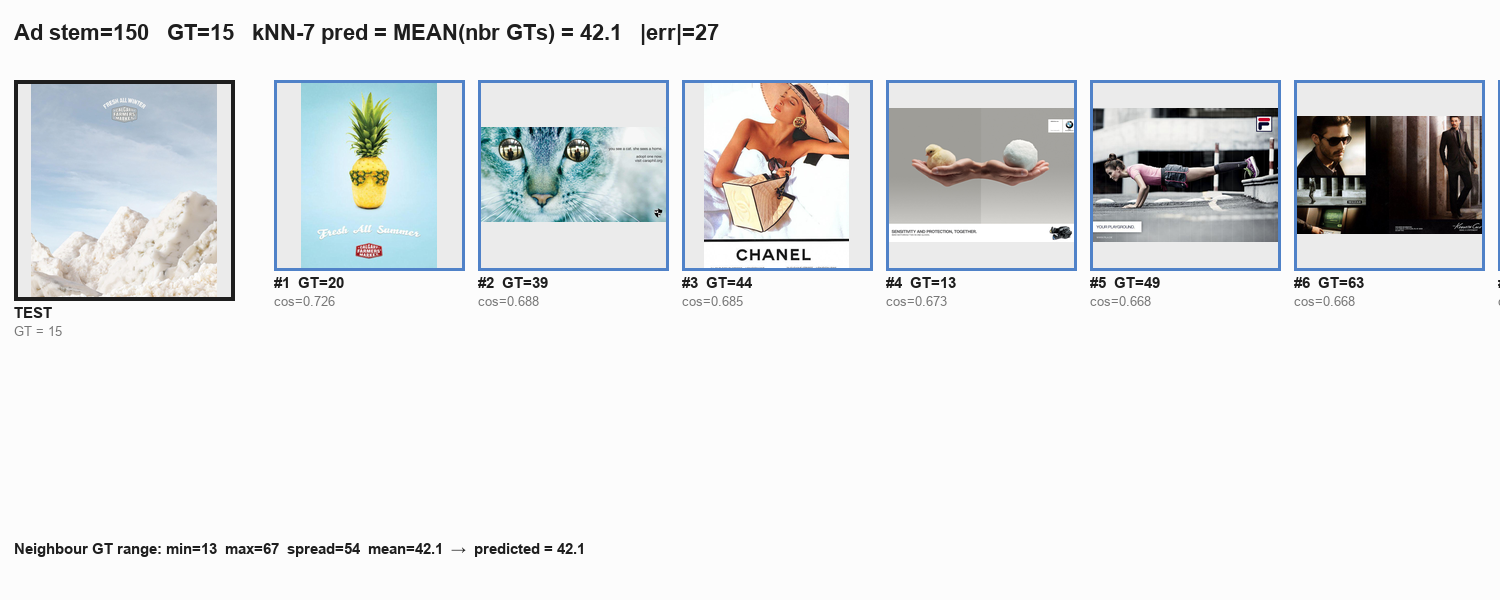
Fig 14. Test ad (left, GT = 15) and its 7 nearest CLIP neighbours. Neighbour GTs span 13–67. Mean = 42. Prediction error = 27. CLIP groups by content; complexity is orthogonal.
9. Method 5 — Gemini-as-Judge with Chain of Thought
Now the bigger gun. Send the ad straight to Gemini 2.5 Pro with a chain-of-thought prompt and ask for an integer score on 0–100. No CLIP, no embedding, no training. The model has never seen SAVOIAS.
from google import genai
from PIL import Image

COT_PROMPT = """You are an expert at rating the VISUAL COMPLEXITY of advertisements.

Visual complexity is the PERCEIVED busyness or density of visual information in
the ad — count of distinct objects, amount of text, color variety, edge/pattern
density, overlapping elements.

Rate on a 0–100 scale:
  0   = extremely minimalist (single object, clean background, no/little text)
  50  = average advertisement (a few elements, moderate text)
  100 = extremely cluttered (many overlapping objects, dense text, busy patterns)

Walk through your reasoning step by step:
  1. List the main visual elements you see.
  2. Note text density and color variety.
  3. Note patterns, textures, overlapping elements.
  4. Compare mentally to mid-range ads (50/100).
  5. Decide a final integer score.

Be concise (≤ 8 short sentences).

On the LAST LINE output EXACTLY:
SCORE: <integer 0–100>
"""

client = genai.Client(api_key=API_KEY)
img = Image.open("ad.jpg").convert("RGB")
resp = client.models.generate_content(
    model="gemini-2.5-pro",
    contents=[img, COT_PROMPT],
)
text = resp.candidates[0].content.parts[0].text
# parse: regex 'SCORE\s*[:=]\s*(\d{1,3})'
One call costs about $0.003 and takes ~10–20 s including the reasoning. The CoT lets us audit why Gemini scored what it scored. Below is one card from the experiment — note all five model scores side by side, plus Gemini’s full reasoning text. This particular ad (a CHANEL split-panel) shows the most interesting disagreement: humans rated it 52 (mid-complexity); Gemini rated it 30, correctly noting the minimalist negative space; CLIP-based methods are all over the map.
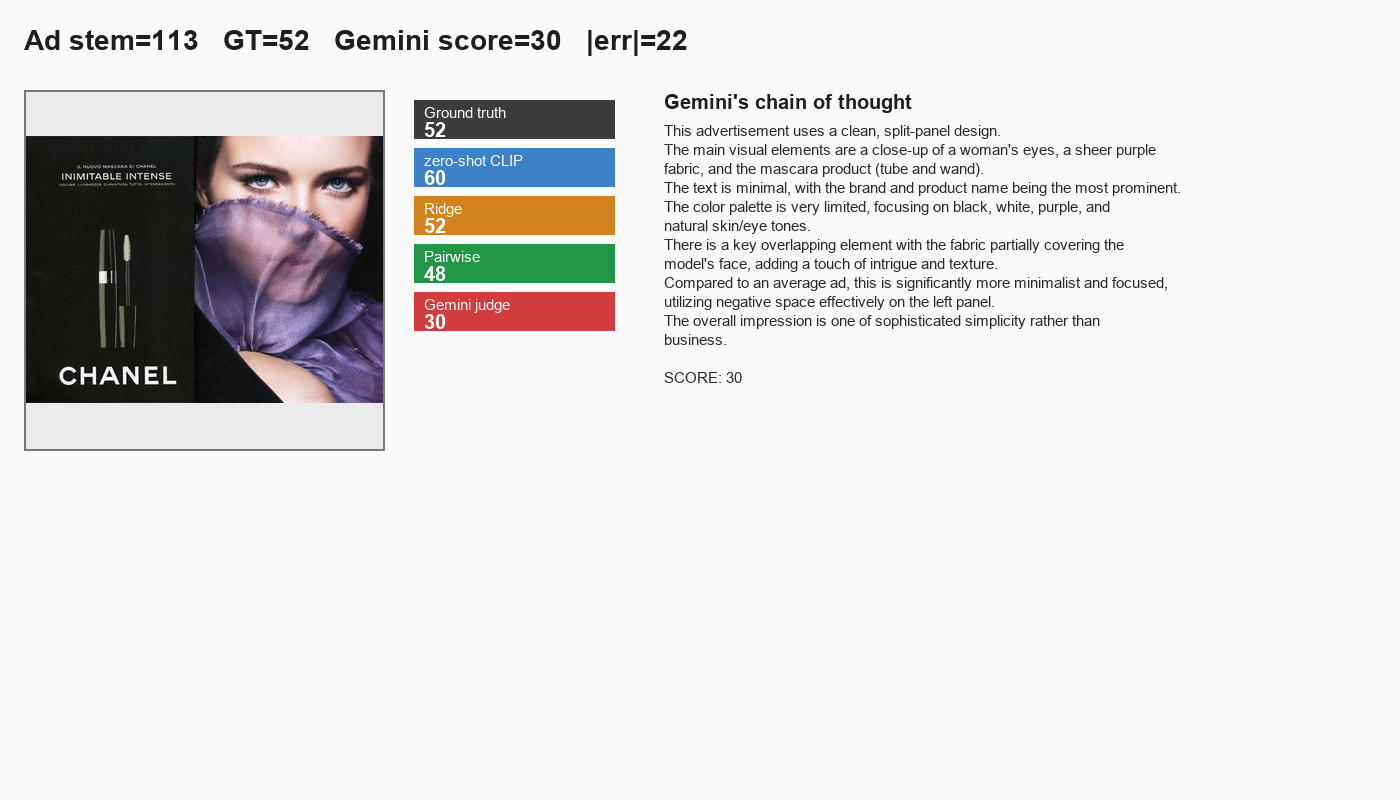
Fig 15. Per-ad card for the CHANEL mascara split-panel ad. GT = 52, Gemini = 30, |err| = 22. Gemini’s reasoning correctly identifies the minimalist design language; the SAVOIAS raters weighted the woman’s face and the bold contrast more heavily. Where Gemini disagrees with humans, the disagreement is usually interpretable.
10. Few-Shot Gemini — Does Calibration Help?
Reasonable next question: if we hand Gemini six reference ads with their known GTs before showing it the test ad, does it score the test ad better? In other words, does in-context calibration help an already-strong model?
We pick 6 calibration anchors from the 190 non-test ads at target GTs \([10, 30, 45, 60, 75, 90]\), then send all 7 images (6 anchors + 1 test) in a single multimodal prompt and ask Gemini to interpolate.
contents = [FEWSHOT_PROMPT]
for k, anchor_idx in enumerate(calib_indices, 1):
    anchor_img = Image.open(df.iloc[anchor_idx]["path"]).convert("RGB")
    contents.append(f"REFERENCE #{k} — known complexity score = "
                     f"{y[anchor_idx]:.0f}/100")
    contents.append(anchor_img)

contents.append("NEW advertisement to rate:")
contents.append(Image.open(test_path).convert("RGB"))
contents.append(NEW_QUERY_INSTRUCTION)

resp = client.models.generate_content(model="gemini-2.5-pro", contents=contents)
The honest answer is: no improvement on this set. On the 10 test ads, zero-shot Gemini gets MAE 9.2 and SROCC 0.87; few-shot Gemini with 6 anchors gets MAE 9.4 and SROCC 0.85. Five ads improved with the anchors, five got worse:
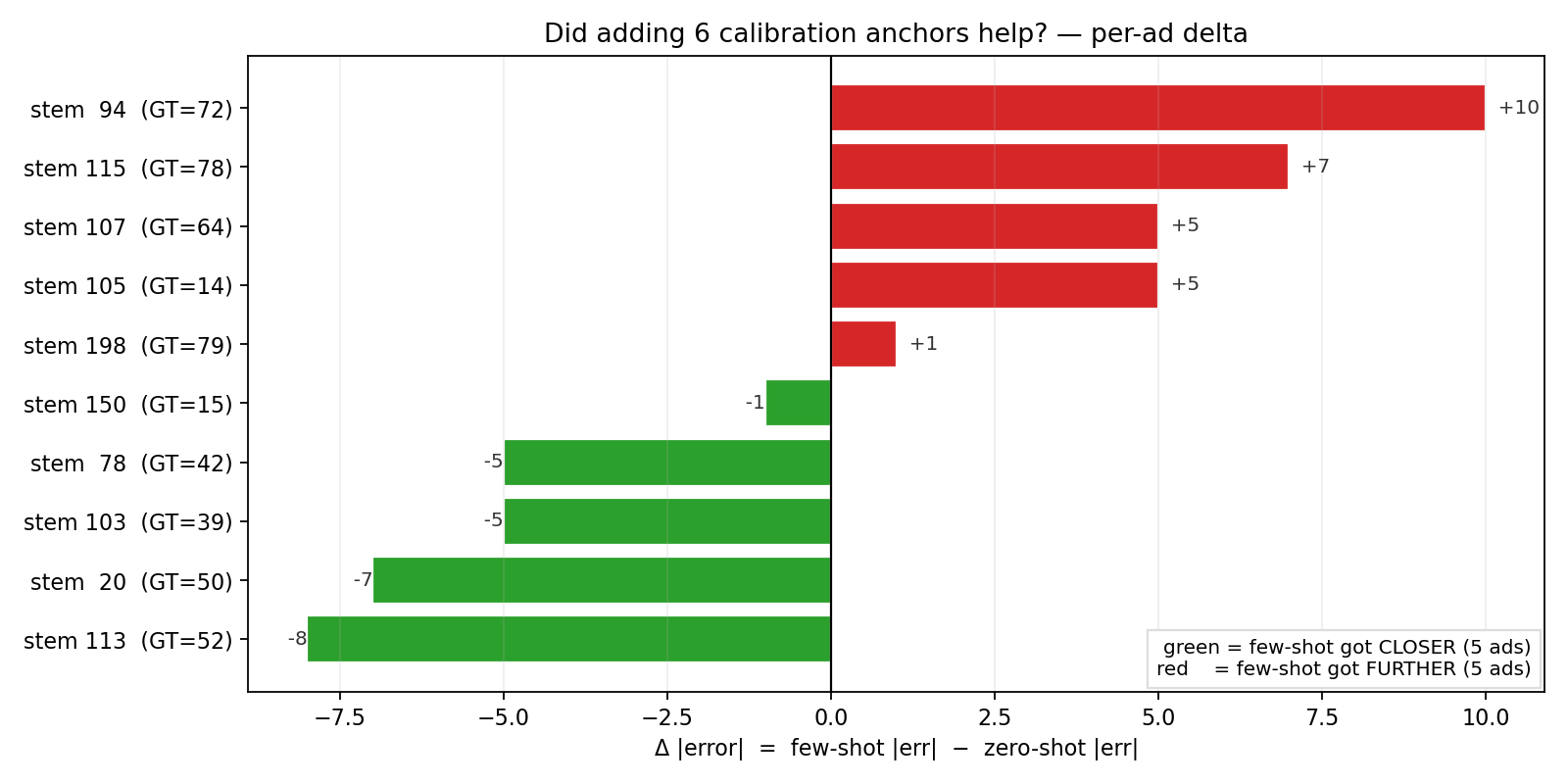
Fig 16. Per-ad change in absolute error after adding 6 calibration anchors to the prompt. Green = few-shot got closer to GT; red = further. Five and five. Mean Δ|err| = +0.2 (slight regression).
The interpretation: Gemini’s internal complexity scale already matches SAVOIAS humans closely enough that 6 anchors add noise as often as signal. Calibration helps when the model is miscalibrated; here it is not.
11. The Honest Held-Out Scoreboard
Same 10 ads, same GTs, every method evaluated with no leakage. Ridge and pairwise are retrained on the 190 non-test ads. Gemini runs zero-shot on each test ad with no prior context. kNN-7 retrieves only from the 190-ad pool.
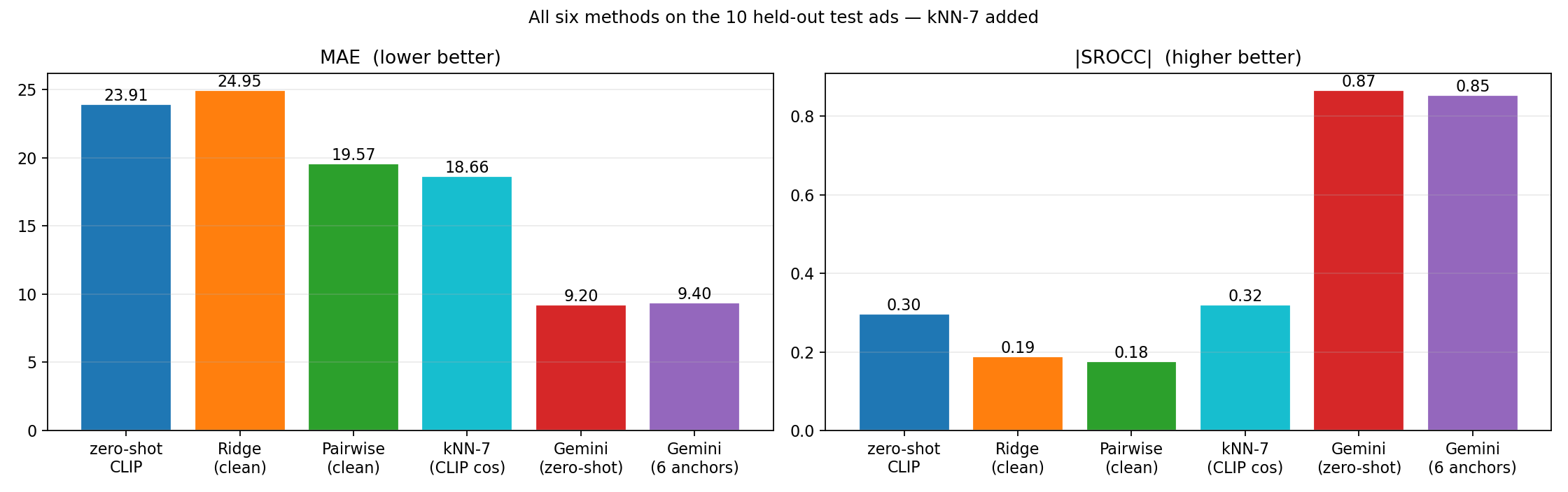
Fig 17. Held-out comparison across six methods on 10 test ads. Left = MAE (lower better), right = |SROCC| (higher better). Gemini wins both, by a wide margin.
| Method | MAE | RMSE | |SROCC| | PLCC |
|---|---|---|---|---|
| Zero-shot CLIP (two prompts) | 23.9 | 28.9 | 0.30 | +0.40 |
| Ridge regression (clean 190/10) | 25.0 | 27.0 | 0.19 | −0.12 |
| Pairwise on Δ-embeddings (clean 190/10) | 19.6 | 21.3 | 0.18 | +0.42 |
| kNN-7 on CLIP cosine | 18.7 | 20.5 | 0.32 | +0.47 |
| Gemini 2.5 Pro (zero-shot CoT) | 9.2 | 11.5 | 0.87 | +0.87 |
| Gemini 2.5 Pro (6 anchors, few-shot) | 9.4 | 11.3 | 0.85 | +0.87 |
Read this carefully. The four classical methods cluster in the MAE 18–25 / |SROCC| 0.18–0.32 range — all far worse than the headline numbers we’d have reported with leakage. Gemini lands in MAE 9 / |SROCC| 0.87. A small caveat: 10 test ads is a small sample and SROCC estimates have wide variance at this scale. The qualitative ordering (Gemini ≫ all CLIP methods) is robust; the exact numbers are not.
12. Why CLIP-Based Methods Fail (Semantic ≠ Complexity)
The kNN visualisation (Fig 4) is the cleanest evidence. CLIP organises its 768-d image space by subject matter — “car ads”, “perfume ads”, “ads with a face on a white background”. Visually similar ads from CLIP’s perspective span the full complexity range. The complexity axis is simply not a direction in CLIP space.
That single observation explains why every classical recipe fails:
- Zero-shot prompts rely on CLIP’s text-aligned axis matching the human notion of complexity. It doesn’t — bold-headline ads register as “complex” even when their layout is empty.
- Ridge regression tries to find a single linear weight \(\mathbf{w}\) such that \(\mathbf{w} \cdot \mathbf{x}\) predicts complexity. Such a weight does not exist when the signal is not linearly extractable.
- Pairwise on differences is more expressive than Ridge but still searches for a single linear ranking direction. On a held-out set it generalises about as well as Ridge.
- kNN retrieval assumes “visually similar in CLIP space ⇒ similar in complexity”. The premise fails for the reason above.
Gemini, in contrast, looks at the actual pixels with its own visual encoder, can read the text on the ad, and produces a token-by-token explanation of what it sees. It does not need to project complexity onto CLIP’s pre-existing axes because it never visits them.
13. The Honest Tournament Test, and Implications
The §7 walkthrough is honest about how the tournament estimator works, but the 0.84 SROCC it advertises was produced with the classifier trained on pairs sampled from all 200 ads — the same partial leakage that flattered Ridge in §5 and pointwise pairwise in §6. The natural follow-up question — does the tournament rescue CLIP-difference when the classifier itself is trained honestly? — needs its own experiment. So we ran one (exp7b):
- Train the pairwise classifier on 3 000 pairs sampled only from the 190 non-test ads (same protocol as §6).
- For each of the 10 held-out test ads, run M = 20 random K = 20-anchor tournaments against anchors drawn from those same 190 ads.
- Average the per-round predictions, score against GT.
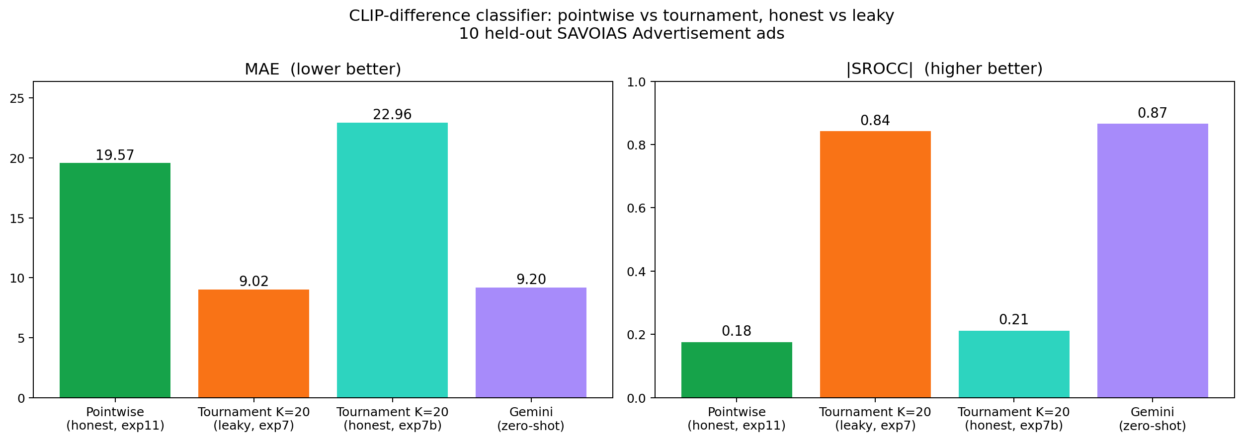
Fig 18. The honest tournament collapses. Pointwise use of the pairwise classifier on a clean 190/10 split (green, exp11) — SROCC 0.18. The leaky tournament (orange, exp7) — SROCC 0.84, but the classifier saw the test ads at train time. The honest tournament (teal, exp7b) — same architecture, classifier retrained on 190 non-test ads — SROCC 0.21. Gemini (purple) — SROCC 0.87. The tournament did not rescue the CLIP-difference signal; the 0.84 was 100% classifier leakage.
Pair-classification accuracy of the honest classifier on test-only pairs is 0.595 — barely above the 0.5 coin-flip baseline. There is nothing for the tournament to amplify. Both ways of using the CLIP-difference classifier (pointwise score, tournament discriminator) collapse on this category.
Does the architecture work where the backbone does have signal?
That collapse is specific to Advertisement. Stage 1 of this project already showed that on the other SAVOIAS category — Interior Design — the CLIP signal is genuinely there: zero-shot CLIP gets SROCC 0.69 (vs 0.55 on Ads) and Ridge regression hits 0.79 (vs 0.38). The natural question: does the honest tournament also survive there? Same script (exp7d) — train classifier on 85 non-test interior images, run K=20 tournaments against random anchors for 15 held-out test images.
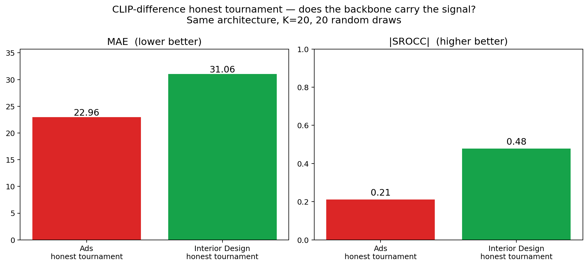
Fig 18b. The honest tournament on Interior Design vs Advertisement, same architecture, K=20. Pair-classification accuracy: 0.685 on Interior Design (decisively above the 0.5 baseline) vs 0.595 on Ads. Tournament SROCC: 0.43 on Interior Design (modest but real, simple-win-rate variant) vs 0.21 on Ads. The architecture is not broken — it carries the signal that the backbone makes available, and CLIP carries enough complexity signal for interior images that the tournament recovers a usable (if not Gemini-tier) ranking.
So the architecture is partially vindicated. On Interior Design, the honest tournament recovers SROCC 0.43 with MAE 13.85 on 15 held-out images — small sample, wide error bars, but a real positive signal. The discriminator’s pair accuracy is 0.685, meaningfully above chance. CLIP-difference can carry complexity, just not on the Ads category where layout text dominates the embedding.
What this means for the original LLM-pairwise pipeline plan:
- The “train a pairwise classifier on CLIP-Δ” half of the plan is falsified for this category. Pairwise on CLIP differences works only when the classifier has already seen the test items at train time. Both pointwise and tournament uses inherit that limitation, because both ride on the same underlying discriminator.
- The replacement plan is simpler: just ask Gemini directly. At $0.003 per image and ~15 s of latency, scoring a 10 000-image packaging catalogue costs $30 and runs in a few hours. No embedding cache, no calibration set, no train/test ceremony.
- If you genuinely cannot send the image to a hosted LLM (privacy, latency, regulatory), the tournament architecture is still the right shape — but the SROCC you get is bounded by how much complexity signal the backbone carries on your specific domain. We measured this for you on SAVOIAS: 0.21 on Advertisement (don’t ship), 0.43 on Interior Design (modest but real). For a new domain, the cheap diagnostic is to train the classifier honestly and check pair-classification accuracy on held-out pairs first. Above ~0.70 the tournament will likely produce a usable ranking; below ~0.62 it will collapse. Further candidates worth trying when CLIP is the bottleneck: the pre-projection 1024-d CLIP feature, DINOv2 / SigLIP embeddings, or a CLIP head fine-tuned on LLM-labelled pairs from the target domain.
14. Summary
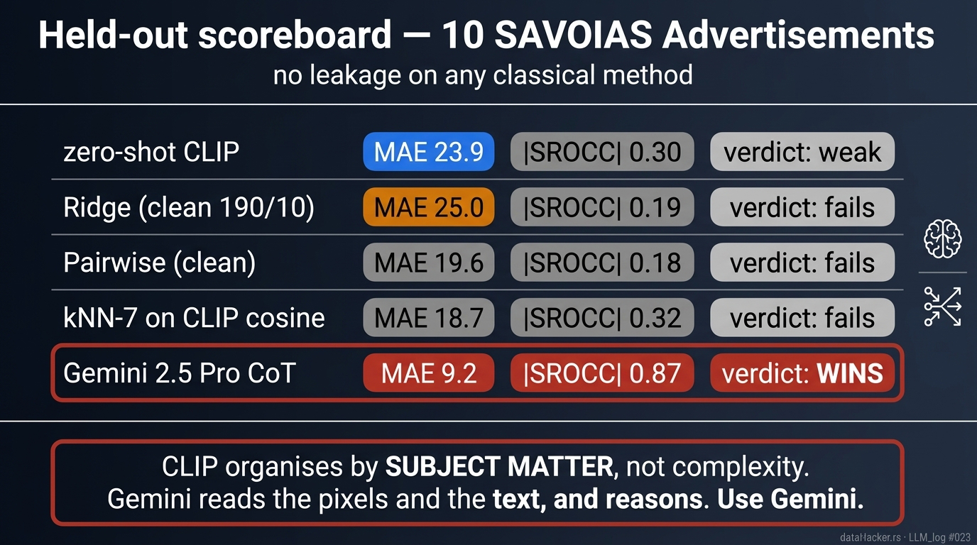
Fig 19. The held-out scoreboard at a glance. Four CLIP-based methods cluster around MAE 19–25 / |SROCC| 0.18–0.32 once the leakage is removed. Add the honest tournament from §13 and it lands in the same cluster (MAE 23 / |SROCC| 0.21). Gemini 2.5 Pro with a one-shot chain-of-thought prompt lands at MAE 9.2 / |SROCC| 0.87 — the only method good enough to ship.
Five methods, one dataset, ten honest test ads. Headline rankings:
- Gemini 2.5 Pro CoT — MAE 9.2, |SROCC| 0.87. Off the shelf, no training, no embeddings.
- Everything CLIP-based — MAE 18.7–25.0, |SROCC| 0.18–0.32 on truly held-out ads. The 0.78 pairwise pointwise number from the deep-dive was leakage; on a clean 190/10 split it drops to 0.18. The 0.84 tournament number was also leakage (the classifier had seen the test ads at train time); rerun honestly (exp7b, §13), the tournament drops to 0.21. CLIP-difference does not separate complexity on this category, regardless of how you use the classifier.
- Few-shot anchors don’t improve Gemini — it’s already calibrated.
- kNN-7 fails because CLIP groups by content, not complexity — neighbours of a simple sky ad include both other minimalist scenes and dense studio shots, mean regresses to the population.
For practical visual-complexity scoring on advertisements: skip the CLIP pipeline. Send the image to an LLM judge. Audit the chain-of-thought when the score surprises you. Calibrate only if the population mean is clearly off — for SAVOIAS ads it is not.
Code, cached embeddings, all five method scripts, and the full 28-page deep dive PDF are in the repository associated with this post. Total compute: about 4 minutes on an M2 MPS device plus 20 Gemini API calls (≈ $0.06).
dataHacker.rs — LLM_log #023 — Visual Complexity Scoring — Vladimir Matic. CLIP via open_clip; LLM judge via Gemini 2.5 Pro.