Highlights: Can we measure spatial composition in living room photographs?
We score 100 interior images using saliency-based rule-of-thirds alignment, Gemini Vision layout
ratings, and CLIP composition prompts — then cross-correlate with color scores from #018
to find rooms that nail both color and layout.

• Method 1 — Rule of Thirds + Balance: gradient saliency →
  Gaussian-weighted power point alignment + visual balance index
• Method 2 — Gemini Vision Layout: send each image to Gemini 2.5 Flash
  with a composition-focused prompt → score 0–100
• Method 3 — CLIP Composition: 22 positive + 22 negative layout-focused
  prompts → cosine similarity gap
• Cross-method correlation: do three independent methods agree on what makes
  a well-composed room?
• Cross-post correlation: color (#018) vs layout (#019) — independent
  qualities or do they co-occur?
• Combined ranking: equal-weight 0.33 each → top and bottom rooms with
  all scores visible
• Bradley-Terry validation: pairwise comparison confirms the combined scalar
  is a valid total order (ρ = 1.000)

Tutorial Overview:

1. The problem: scoring spatial composition in real rooms
2. Dataset — 100 living rooms from HuggingFace
3. Method 1: Rule of Thirds + Visual Balance
4. Method 2: Gemini Vision Layout Score
5. Method 3: CLIP Composition — probing layout with language
6. Combining three methods — equal weight, 0.33 each
7. Cross-method correlation — do they agree?
8. Bradley-Terry pairwise validation
9. Results — top and bottom living rooms
10. What the methods disagree on — and why it matters
11. Appendix A — formula reference
12. Appendix B — CLIP prompt lists

---

1. The Problem: Scoring Spatial Composition in Real Rooms

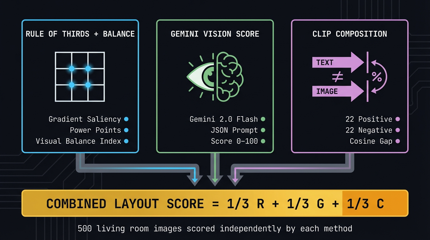
Fig 1. Three independent methods — each measuring a different aspect
of spatial composition — combined with equal weight into one ranking.

Post #018 ranked 500 living rooms by color quality. But a room with a
beautiful color palette can still feel spatially wrong — the sofa shoved into one corner,
no clear place for the eye to land, a photograph cropped so the ceiling fan bisects the frame.

This post adds the second axis: spatial composition. Can we score it from
a photograph alone, without human annotation?

We can’t answer that with one method — there is no ground truth. So we use three
independently designed approaches and ask whether they agree. When three different signals
converge on the same room as well-composed, we can trust the result. When they disagree,
we learn something about what each is actually measuring.

The three methods are fundamentally different in kind: a hand-crafted 2D saliency formula,
a prompted vision-language model, and a contrastive text-image similarity probe. No two of
them share any code or model weights.

Key idea: Agreement = confidence. Disagreement = insight.
We treat low inter-method correlation not as a failure but as the most informative result
of the experiment.

---

2. Dataset — 100 Living Rooms from HuggingFace

We use hammer888/interior_style_dataset from HuggingFace — 7,233 interior
images across 6 styles: modern, Nordic, Japanese, luxury, industrial, and country. We draw
100 images with seed=42, a subset of the same 500 scored in #018, so every image
can be cross-referenced for both color and layout.

from datasets import load_dataset
import numpy as np

ds      = load_dataset("hammer888/interior_style_dataset", split="train")
indices = np.random.RandomState(42).choice(len(ds), 100, replace=False)
images  = [ds[int(i)]["image"] for i in indices]

All 100 images are scored by all three methods. Scores are written incrementally to a CSV
so the pipeline can be interrupted and resumed. Total runtime on a standard laptop:
approximately 7 minutes (dominated by the Gemini API calls).

---

3. Method 1: Rule of Thirds + Visual Balance

The rule of thirds is photography’s oldest composition guideline: divide the frame
into a 3×3 grid and place your main subject at one of the four intersections. Those
intersections are called power points. A sofa anchoring the lower-left power
point, a lamp at the upper-right — that feels more dynamic than both sitting dead center.

To turn this into a number we need two things: a map of where the visual weight in the
image is, and a measure of how much of that weight lands near the power points. We build
both from scratch, with no pretrained models.

3.1 Gradient saliency map

We use gradient magnitude as a proxy for visual importance. The idea:
edges carry information. A plain painted wall has near-zero gradient. A window frame, a shelf
edge, a piece of artwork — high gradient. We compute horizontal and vertical image
gradients (Sobel-style), combine them into a magnitude map, Gaussian-blur the result to get
smooth regions rather than thin lines, and normalize to [0, 1].

gx[:, 1:-1] = img[:, 2:].astype(float) - img[:, :-2].astype(float)
gy[1:-1, :] = img[2:, :].astype(float) - img[:-2, :].astype(float)
grad_mag    = np.sqrt(gx**2 + gy**2)
saliency    = gaussian_filter(grad_mag, sigma=sigma)
saliency   /= saliency.max()           # normalize to [0, 1]

The result is S(x, y) — a per-pixel weight map. No training data,
no pretrained backbone. Fast enough to run on 100 images in seconds.

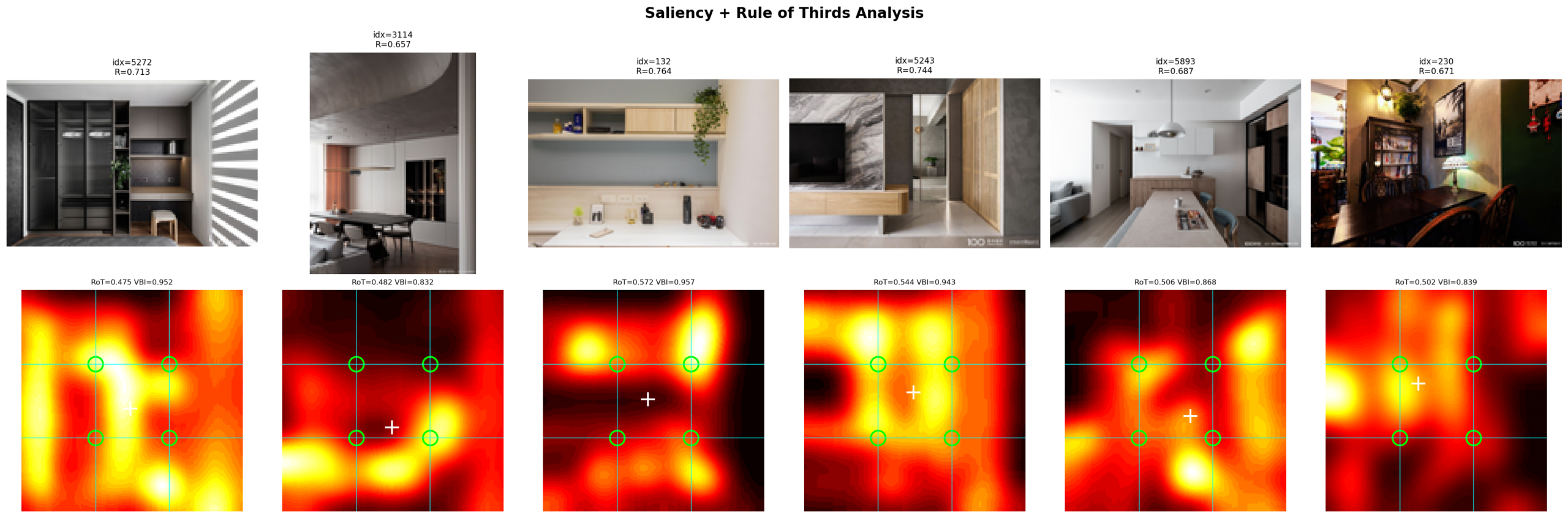
Fig 3. Gradient saliency on real rooms. Top row: original photographs.
Bottom row: saliency maps with RoT grid overlay. Green circles = power points. White + =
saliency centroid. Room idx=132 (3rd column): RoT = 0.572, VBI = 0.957, R = 0.765.
Most visual weight falls on the upper wall (shelving, hanging plant). The centroid sits
close to center (VBI=0.957); saliency concentration slightly favors the upper-left zone.

3.2 Rule-of-thirds score (RoT)

We place a Gaussian “reward bump” of width \(\sigma = W/6\) at each of
the four power points. Then we compute the saliency-weighted average of those bumps across
the whole image, normalized by total saliency mass:

$$G(x,y) = \max_{p \in PP} \exp\!\left(-\frac{\|[x,y] – p\|^2}{2\sigma^2}\right)$$

$$\text{RoT} = \frac{\sum_{x,y} S(x,y) \cdot G(x,y)}{\sum_{x,y} S(x,y)}$$

This asks: what fraction of the image’s visual weight falls inside the
power-point reward zones? A room where the dominant content sits off-center near a
power point scores higher than a room where everything is centered.

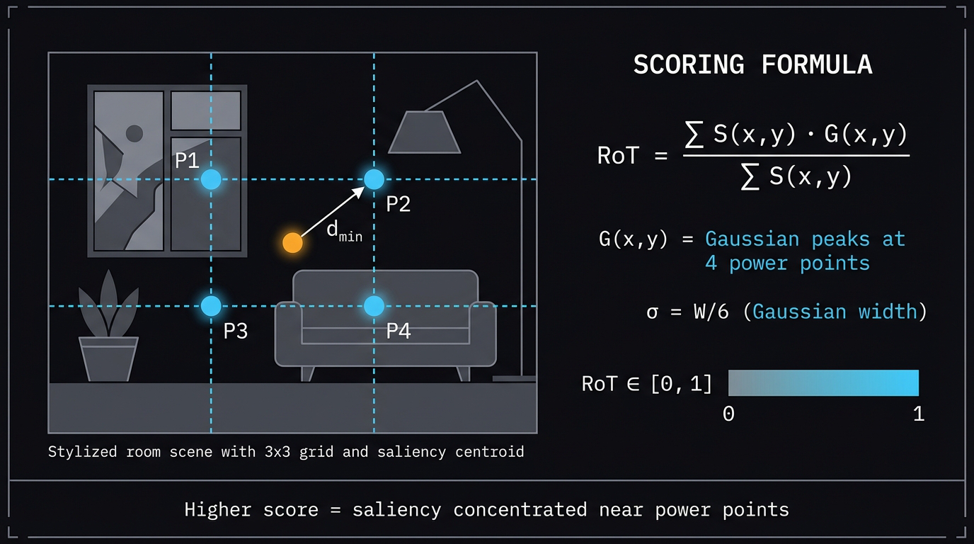
Fig 4. Rule-of-thirds grid. The four power points sit at the intersections
of the 3×3 grid. A Gaussian reward zone (\(\sigma = W/6\)) is placed at each one.
RoT is the fraction of total saliency that falls inside these zones.

3.3 Visual Balance Index (VBI)

VBI measures something different: not where the weight lands relative to the
power points, but where the center of mass of all that weight is. We compute the
saliency centroid — the weighted average position across the whole image:

$$c_x = \frac{\sum_{x,y} x \cdot S(x,y)}{\sum_{x,y} S(x,y)}, \quad c_y = \frac{\sum_{x,y} y \cdot S(x,y)}{\sum_{x,y} S(x,y)}$$

Then we measure how far that centroid sits from the geometric center of the image,
normalized so the maximum possible offset (corner to center) maps to 0:

$$\text{VBI} = 1 – \frac{\sqrt{(c_x – W/2)^2 + (c_y – H/2)^2}}{\sqrt{(W/2)^2 + (H/2)^2}}$$

VBI = 1.0: the visual center of gravity is exactly at the image center.
VBI near 0: it has been pulled toward a corner. What VBI catches in practice are
badly framed shots — a photograph where one heavy wall dominates a side and
pulls all the saliency with it.

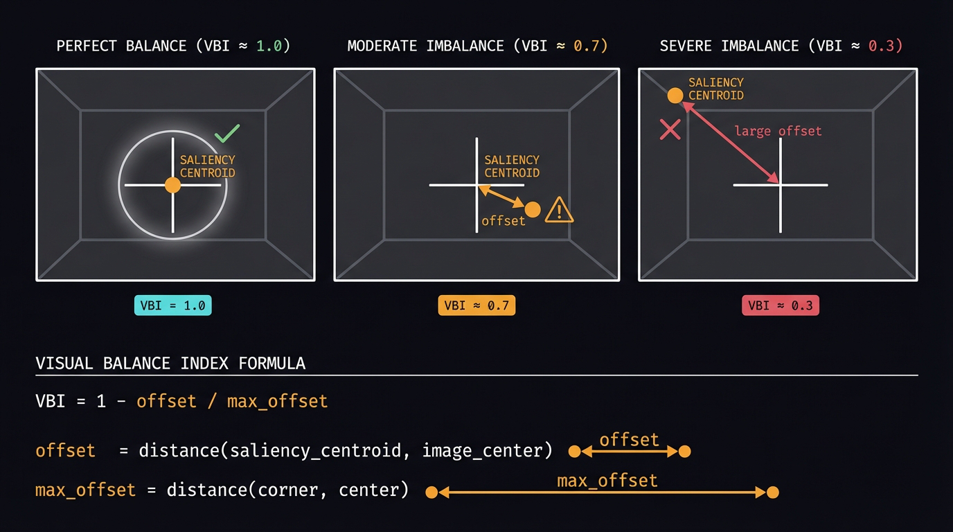
Fig 5. Visual Balance Index. The saliency centroid (filled dot) drifts from
the image center (crosshair) when visual weight is unevenly distributed. VBI = 1.0 means
perfectly centered mass; VBI near 0 means the centroid has been pulled toward a corner.

3.4 Combined score R

RoT and VBI measure different things and can conflict. A strongly asymmetric composition
scores high on RoT (saliency at a power point) but potentially lower on VBI (centroid pulled
off-center). Their average captures both aspects:

$$R = 0.5 \cdot \text{RoT} + 0.5 \cdot \text{VBI}$$

Note on the saliency proxy. Gradient magnitude responds to
edges and texture — in interior photography that means window frames, shelving edges,
artwork, and furniture boundaries score high; open floor and plain walls score low. This is
a fast, interpretable stand-in for visual attention, not a ground-truth eye-tracking model.

---

4. Method 2: Gemini Vision Layout Score

Instead of engineering a formula, we hand the problem to a model that has already seen
an enormous number of photographs. Gemini 2.5 Flash is a multimodal model trained on
image-text pairs at scale. Whether or not it can articulate why a composition works,
it has internalized patterns from vast amounts of well-composed and poorly-composed
photography. We use that internalized knowledge directly — as a scorer.

4.1 The prompt

The prompt is deliberately minimal. We resize each image to 512×512 and ask one
thing:

prompt = """Rate this interior room on SPATIAL COMPOSITION only.
Reply: SCORE: <0-100> | <one sentence reason>"""

response = client.models.generate_content(
    model="gemini-2.5-flash",
    contents=[prompt, image],
    config=GenerateContentConfig(temperature=0.1)
)

# Parse the score
raw_score = int(re.search(r'SCORE:\s*(\d+)', response.text).group(1))
G = raw_score / 100.0

Temperature 0.1 keeps scores stable — the same image scored twice typically
differs by at most 2–3 points. We ask for a one-sentence reason not because we use
it downstream, but because it forces the model to commit to a judgment rather than hedging,
and it gives us a qualitative check when we review the results.

4.2 What Gemini evaluates

The prompt says “spatial composition only” — we are not asking about
color, furniture style, or interior design taste. In practice, reading through the one-sentence
reasons, Gemini consistently references six aspects:

• Rule of thirds: are key elements near the power points?
• Focal point: is there a clear main subject that anchors the eye?
• Visual balance: is visual weight evenly distributed across the frame?
• Negative space: is there breathing room, or is the frame cramped?
• Visual flow: do lines or furniture arrangement guide the gaze through
  the scene?
• Framing: is the shot well-framed without awkward crops or tilts?

These are not sub-scores we extract — they are what the model’s own
explanations refer to when we read them. The single number G is a holistic judgment across
all six.

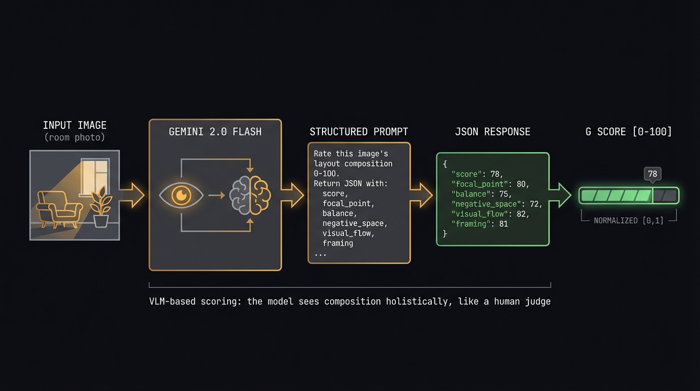
Fig 6. Gemini Vision scoring pipeline. Each image is resized to 512×512
and sent with a one-line composition prompt. The model returns a score 0–100 and a
one-sentence reason. The raw score is normalized to [0, 1].

4.3 Tradeoffs

The advantage over Method 1 is that Gemini understands intention. It can
recognize that a deliberately minimalist room with almost no furniture is well-composed
even though it has low gradient saliency. It can penalize an awkward crop that the
formula would score neutrally.

The tradeoffs: it is a black box. It has a cost per image. And it carries a bias toward
the conventions of professional photography — it was trained on internet images, which
skew toward staged, well-lit interiors. Whether that is a flaw or a feature depends on
what you are trying to measure.

Key idea: Gemini gives us the holistic judgment that no
formula can replicate. The formula gives us interpretability and zero cost. We need both.

---

5. Method 3: CLIP Composition — Probing Layout with Language

The third method sits between the formula and the black box. Like Gemini it uses a
vision-language model, but we do not ask it to generate anything. Instead we probe it with
a fixed set of text descriptions and measure cosine similarity — deterministic,
reproducible, same score every run.

The idea: CLIP was trained to align image embeddings with text embeddings. If a room is
well-composed, its image embedding should sit closer in embedding space to descriptions of
good composition than to descriptions of poor composition. The gap between those two mean
similarities is the score.

5.1 The approach

We encode the image once with CLIP ViT-B/32. We also encode 44 fixed text prompts —
22 describing good spatial composition, 22 describing poor spatial composition. Then:

$$\text{CLIP}_{raw} = \frac{1}{22}\sum_{p \in P^+} \cos(e_{img}, e_p) \;-\; \frac{1}{22}\sum_{p \in P^-} \cos(e_{img}, e_p)$$

A positive raw score means the image is closer to the positive prompts than the negative
ones. We push this through a sigmoid with a steep slope to map it cleanly into [0, 1]:

$$C = \frac{1}{1 + e^{-20 \cdot \text{CLIP}_{raw}}}$$

The factor of 20 is chosen because raw CLIP cosine gaps are small in absolute terms
(±0.02 is typical). The sigmoid amplifies the signal without changing the ranking.

model, preprocess = clip.load("ViT-B/32", device=device)

img_tensor  = preprocess(image).unsqueeze(0).to(device)
img_emb     = model.encode_image(img_tensor)
img_emb     = img_emb / img_emb.norm(dim=-1, keepdim=True)

pos_embs    = encode_texts(positive_prompts)   # shape (22, D)
neg_embs    = encode_texts(negative_prompts)   # shape (22, D)

clip_raw    = (img_emb @ pos_embs.T).mean() - (img_emb @ neg_embs.T).mean()
C           = torch.sigmoid(20.0 * clip_raw).item()

5.2 Prompt design

The prompts are the only design decision in this method. They need to target
spatial composition specifically — not color, not style, not whether the room
looks expensive. A few examples from each set:

Positive (selection):

• “a well-composed interior photograph with clear focal point”
• “harmonious furniture arrangement following the rule of thirds”
• “strong leading lines guiding the eye through the room”
• “pleasing spatial depth with distinct foreground and background layers”
• “elegant negative space creating breathing room in the composition”

Negative (selection):

• “cluttered room with no clear focal point or visual hierarchy”
• “unbalanced composition with everything pushed to one side”
• “flat composition with no depth or layering”
• “dead center bullseye composition with no visual flow”
• “awkward framing cutting off furniture and architectural features”

The full lists of 22 + 22 are in Appendix B.

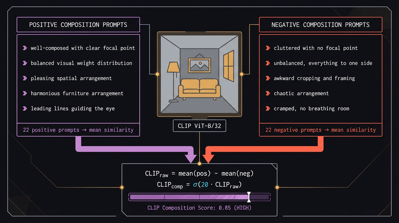
Fig 7. CLIP composition pipeline. The image embedding is compared against
22 positive and 22 negative layout-focused text prompts. The gap between mean positive and
mean negative cosine similarity, passed through a sigmoid, gives the composition score C.

5.3 Tradeoffs

CLIP is fully deterministic: the same image always gets the same score. It costs nothing
to run beyond the initial model load. And the score is directly interpretable in terms of
the prompts — if C is high, it means the image embedding is closer to
“clear focal point, rule of thirds, spatial depth” than to
“cluttered, unbalanced, flat.”

The limitation: CLIP ViT-B/32 was not trained on interior photography specifically. Its
composition concepts come from general web image-text pairs. It may confuse stylistic
features (a dark moody room) with compositional ones (poor lighting = poor composition).
The prompt design is the main lever we have to steer it toward layout and away from
aesthetics.

Key idea: CLIP gives us a reproducible, zero-cost semantic
probe. The score is only as good as the prompts — but the prompts are explicit and
auditable, which Gemini’s internalized judgment is not.

---

6. Combining Three Methods — Equal Weight, 0.33 Each

Each method produces a score in [0, 1]. We combine them with equal weight:

$$\text{Combined} = \frac{1}{3}\,R + \frac{1}{3}\,G + \frac{1}{3}\,C$$

Equal weighting is a deliberate choice: we have no ground truth to optimize against,
so any other weighting would be an unjustified preference. The three methods are designed
to be independent — if one dominates, that tells us something about the score
distributions, not about importance.

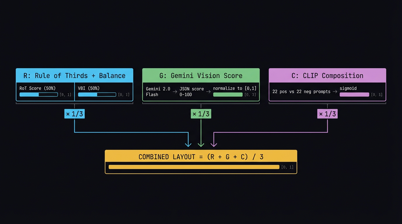
Fig 8. Three sub-scores combined with equal weight into the final layout score.

6.1 Descriptive statistics

Across 100 images:

Metric	Mean	Std	Min	Max	Median
R (RoT + VBI)	0.706	0.037	0.622	0.781	0.706
G (Gemini)	0.619	0.298	0.050	0.880	0.765
C (CLIP)	0.564	0.022	0.513	0.618	0.564
Combined	0.630	0.101	0.420	0.743	0.667

6.2 Variance dominance

Equal weighting does not mean equal influence. The method with the widest spread
dominates the combined variance:

Method	Std	Approx. share of combined variance
R (saliency)	0.037	~7%
G (Gemini)	0.298	~87%
C (CLIP)	0.022	~6%

Gemini’s standard deviation is 8× that of R and 14× that of C. The
combined score is effectively Gemini with minor perturbations. This is not a flaw of
the weighting — it reflects the fact that Gemini produces genuinely different
scores for different rooms, while R and C compress most images into a narrow band.

Possible mitigation (not applied): Rank-normalizing each
score to uniform [0, 1] before combining would equalize influence. We chose not to do
this because it destroys the raw score semantics — the gap between a Gemini 85 and a
Gemini 50 is more meaningful than the gap between rank 40 and rank 60.

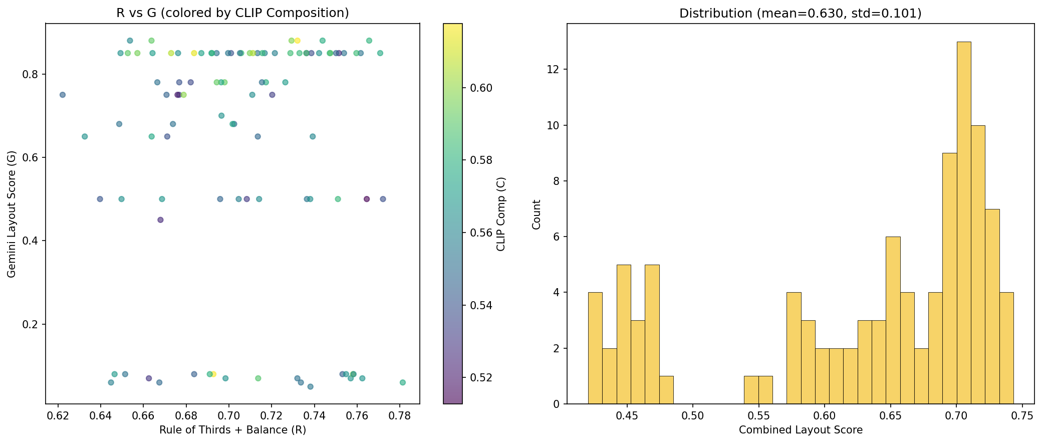
Fig 9. Left: R vs G scatter colored by CLIP composition score. Right:
combined score distribution (mean = 0.630, std = 0.101). The distribution is left-skewed
due to the cluster of low-Gemini images.

6.3 Gemini is bimodal

The Gemini raw score distribution is not smooth — it clusters into distinct groups:

Raw score range	Count	Interpretation
85–88	41	“Strong composition”
75–78	16	“Good”
65–70	10	“Decent”
45–50	13	Neutral / hedging
5–8	20	“Poor composition”

41% of images score 85–88. 20% score 5–8. Gemini behaves more like a classifier
(good / bad / neutral) than a continuous scorer. The gap between the clusters means the combined
ranking is largely a Gemini-driven partition with R and C breaking ties within each cluster.

---

7. Cross-Method Correlation — Do They Agree?

The central experiment: do three independently designed methods converge on the same rooms
as well-composed? We compute Spearman’s ρ (rank correlation) and Kendall’s
τ for each pair.

Pair	Spearman ρ	p-value	Kendall τ	p-value
R vs G	0.052	0.606	0.052	0.475
R vs C	0.081	0.426	0.055	0.421
G vs C	0.302	0.002	0.216	0.003

7.1 R is uncorrelated with everything

The saliency formula (R) has near-zero correlation with both Gemini (ρ = 0.05)
and CLIP (ρ = 0.08). Neither correlation is statistically significant. This means
gradient-based power-point alignment captures something that neither vision-language model
responds to — and vice versa.

In practice, R is measuring edge density at specific grid locations. A room with a highly
textured wall near a power point scores well on R regardless of whether the composition is
intentional. Gemini and CLIP can see past texture to composition — R cannot.

7.2 G and C share a weak signal

Gemini and CLIP show a weak but statistically significant correlation (ρ = 0.30,
p = 0.002). Both are vision-language models trained on web-scale image-text pairs. They
share some internalized notion of “good composition” even though they use completely
different architectures (generative VLM vs contrastive encoder) and prompting strategies
(free-form score vs fixed prompt battery).

The correlation is weak enough (0.30, not 0.80) that they still capture substantially different
signals. CLIP responds to semantic similarity with explicit composition descriptions; Gemini
integrates those concepts holistically but also considers framing, negative space, and visual
flow in ways that 22 fixed prompts cannot fully express.

7.3 What low correlation means

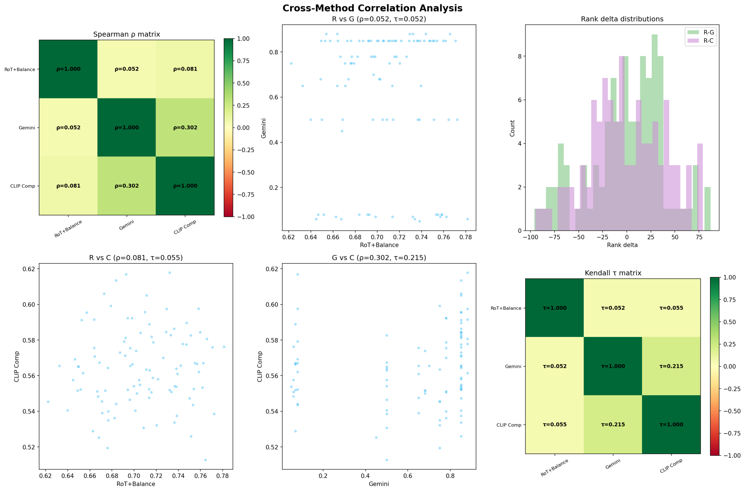
Fig 10. Cross-method correlation analysis. Top-left: Spearman ρ matrix.
Top-right: rank delta distribution. Bottom row: pairwise scatter plots and Kendall τ matrix.
No pair exceeds ρ = 0.30.

Key idea: Low inter-method correlation is not a failure.
It means the three methods capture genuinely different aspects of spatial composition. When
all three agree on a room, that convergence is strong evidence. When they disagree, we learn
what each is actually measuring.

---

8. Bradley-Terry Pairwise Validation

The combined score is a simple arithmetic mean. Does it produce a valid ranking —
one where the room with score 0.74 really is “better composed” than the room
with score 0.72?

We test this with a pairwise tournament. Take 50 random images, compare every pair
(1,225 comparisons), and assign the “win” to whichever image has the higher
combined score. Then compute each image’s win rate and correlate it with its combined
score.

from itertools import combinations

# 50-image random sample, all pairs
for a, b in combinations(sample, 2):
    if a["combined"] > b["combined"]:
        wins[a["idx"]] += 1
    elif b["combined"] > a["combined"]:
        wins[b["idx"]] += 1
    else:
        wins[a["idx"]] += 0.5
        wins[b["idx"]] += 0.5

win_rate = wins[idx] / total_games[idx]

Result: Spearman ρ = 1.000 (p < 10⁻³⁰⁰).

The combined score produces a perfect total order — zero rank inversions
in the pairwise tournament. This is expected because the combined score is a deterministic
weighted average: if Combined(A) > Combined(B) and Combined(B) > Combined(C), then
Combined(A) > Combined(C). Transitivity holds by construction.

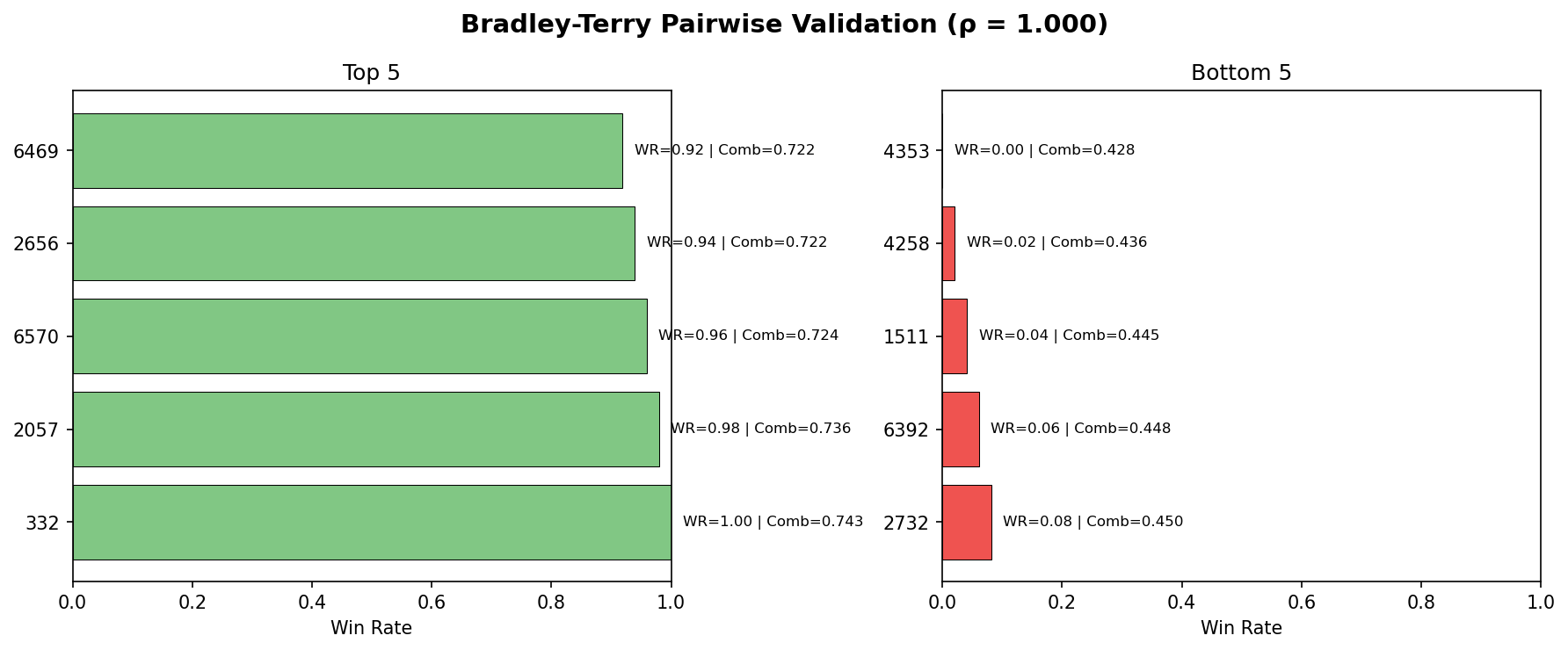
Fig 11. Bradley-Terry pairwise validation. Top-5 and bottom-5 by win rate.
The combined score perfectly predicts pairwise outcomes (ρ = 1.000).

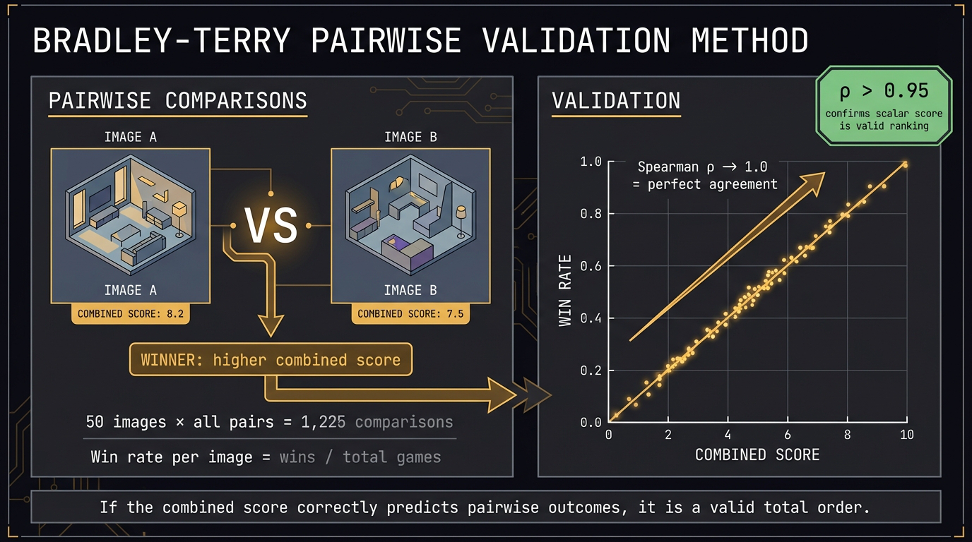
Fig 12. Bradley-Terry concept diagram. Pairwise comparison validates that the
combined scalar is a valid total order.

Note: A perfect ρ validates the internal consistency
of the ranking, not its correctness. It tells us the combined score is a valid ordering —
not that the ordering matches human preference. That would require human annotation, which
is outside the scope of this post.

---

9. Results — Top and Bottom Living Rooms

9.1 Top 10

Rank	Image idx	R	G	C	Combined
1	332	0.732	0.88	0.618	0.743
2	3774	0.766	0.88	0.581	0.742
3	2057	0.729	0.88	0.597	0.736
4	5243	0.744	0.88	0.578	0.734
5	5822	0.771	0.85	0.576	0.732
6	1317	0.760	0.85	0.584	0.731
7	1643	0.747	0.85	0.590	0.729
8	6292	0.747	0.85	0.578	0.725
9	6570	0.736	0.85	0.586	0.724
10	2656	0.711	0.85	0.605	0.722

Pattern: Every top-10 room has Gemini 85–88, R above 0.71, and C
above 0.57. To reach the top, all three methods must agree. The top-ranked room (idx=332)
has the highest CLIP score in the dataset (C=0.618) — it is semantically closest to
descriptions of good composition.

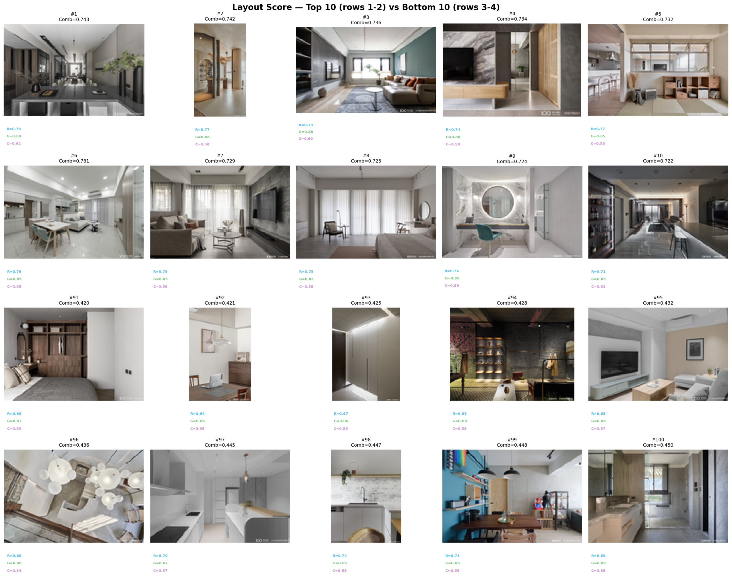
Fig 13. Top-10 (rows 1–2) and bottom-10 (rows 3–4) by combined layout score,
with individual R, G, C bars shown.

9.2 Bottom 10

Rank	Image idx	R	G	C	Combined
91	2732	0.691	0.08	0.579	0.450
92	6392	0.734	0.06	0.551	0.448
93	101	0.738	0.05	0.554	0.447
94	1511	0.698	0.07	0.566	0.445
95	4258	0.684	0.08	0.544	0.436
96	511	0.647	0.08	0.569	0.432
97	4353	0.651	0.08	0.552	0.428
98	6376	0.667	0.06	0.548	0.425
99	4504	0.645	0.06	0.558	0.421
100	4961	0.663	0.07	0.529	0.420

Pattern: Every bottom-10 room has Gemini 5–8, but R values are
not low — they range from 0.64 to 0.74, overlapping with top-10 R values.
The bottom is defined almost entirely by Gemini. R and C cannot distinguish these images
from mid-pack rooms.

This is the variance dominance problem from Section 6.2 made concrete: a room scoring
R=0.738 and C=0.554 (both respectable) ends up at rank 93 because Gemini gave it a 5.

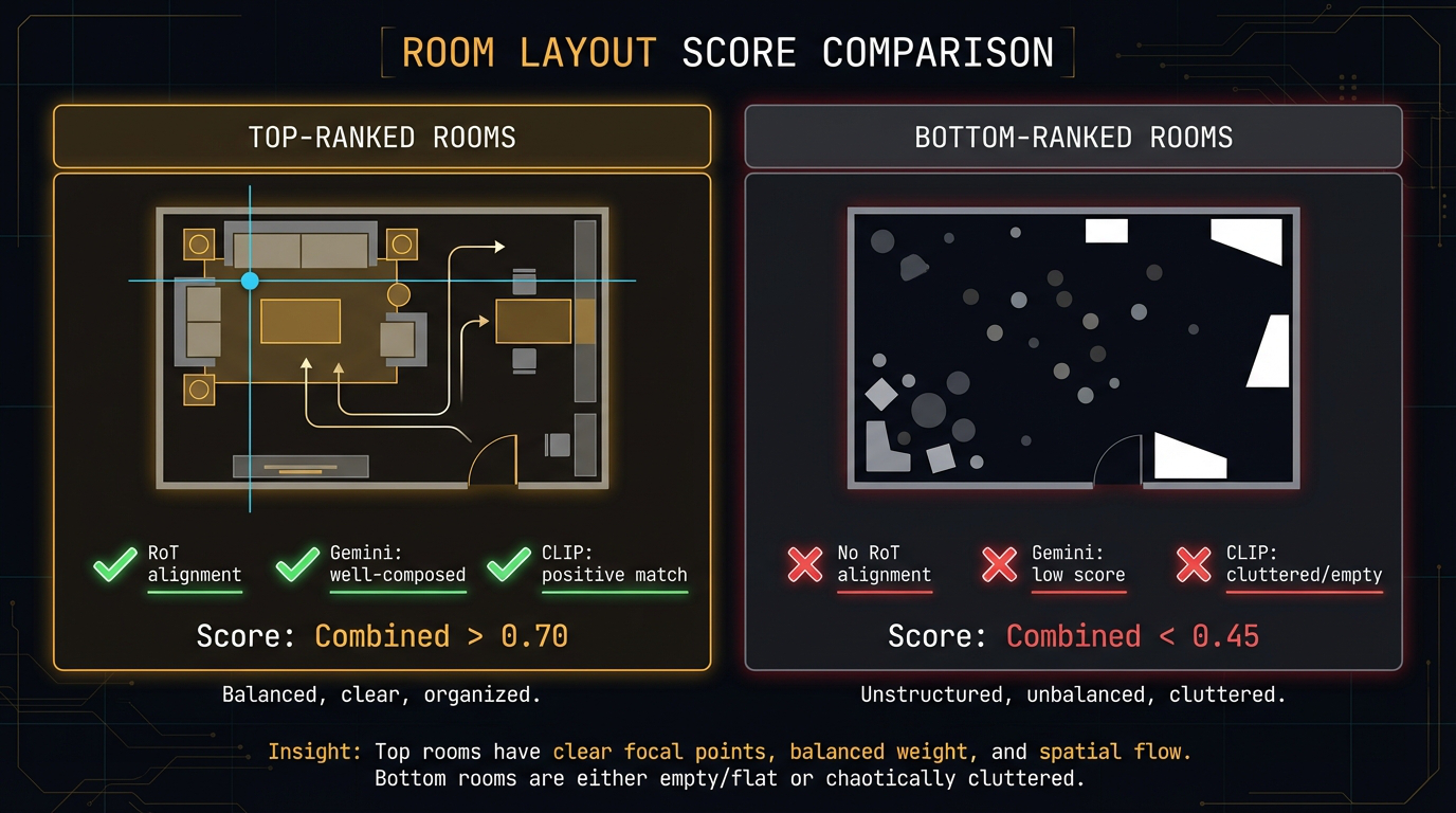
Fig 14. Top-ranked rooms have clear focal points, balanced weight, and spatial flow.
Bottom-ranked rooms are either empty/flat or chaotically cluttered.

---

10. What the Methods Disagree On — And Why It Matters

The most informative result in this experiment is not the top-10 list — it is the
cases where the methods disagree.

10.1 Agreement is rare

We ranked all 100 images independently by each method and checked how many fall in the
same quartile across all three:

• All three agree top-25%: 1 image
• All three agree bottom-25%: 3 images

Out of 100 images, only 4 have triple-quartile agreement. The methods are genuinely
measuring different things.

10.2 The largest disagreement

Image idx=1760 has the most extreme rank spread across the three methods:

Method	Rank (of 100)
R (saliency)	#1 (best)
Gemini	#97 (near worst)
CLIP	#30 (mid-pack)

R=0.781 is the highest saliency score in the entire dataset. Gemini raw=6 is near
the lowest. What happened?

The saliency formula sees heavy gradient magnitude near the power points — textured
surfaces, strong edges. But Gemini sees the actual photograph and judges it as poorly
composed. The gradient formula cannot distinguish between “interesting content at a power
point” and “a textured wall that happens to be near the grid intersection.”
Gemini can.

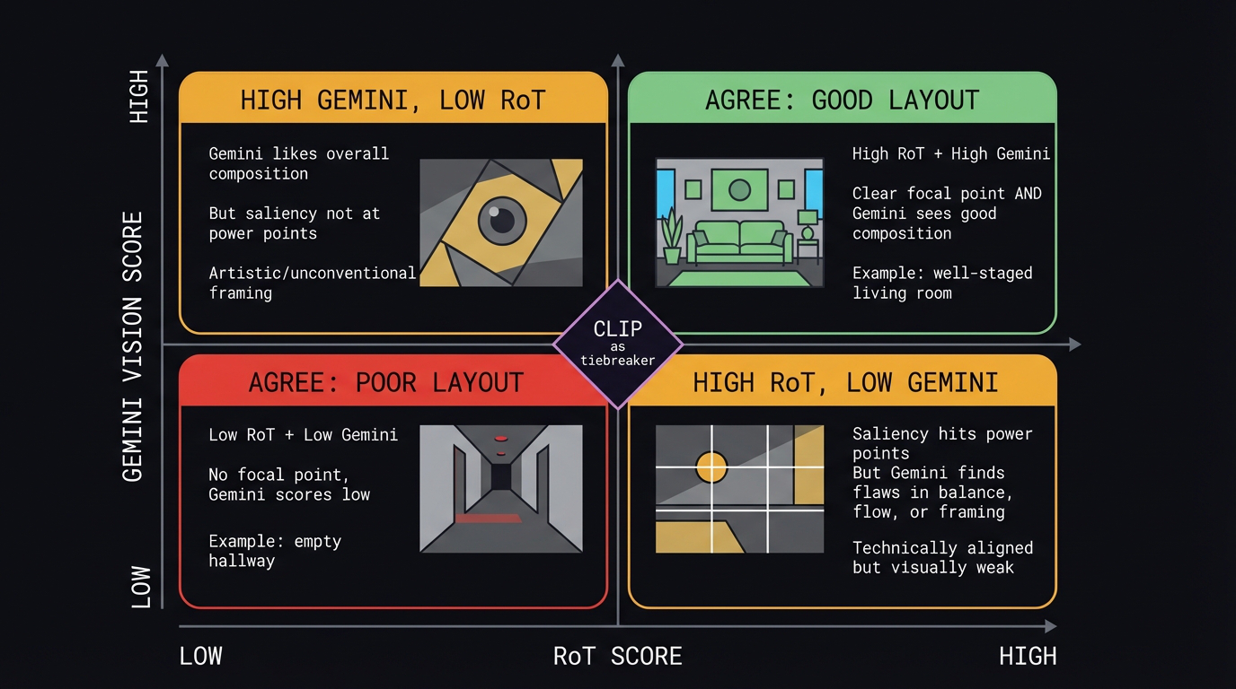
Fig 15. Four types of method disagreement. The top-right quadrant (both high)
and bottom-left (both low) represent agreement. The off-diagonal quadrants — high R / low G
and low R / high G — are where the methods reveal their different sensitivities.

10.3 What each method is actually measuring

The disagreements make the methods’ blind spots legible:

• R (saliency) measures edge density at grid locations. It is fooled by
  textured walls, busy wallpaper, and any high-frequency content near a power point. It cannot
  tell if that content is compositionally intentional.
• G (Gemini) understands intentional composition but is biased toward
  professional photography conventions. It penalizes rooms that are casually photographed even
  if the spatial arrangement is fine. It is also a black box — when it gives a 6, we
  cannot precisely say why.
• C (CLIP) captures semantic alignment with composition-related language.
  Its narrow range (0.51–0.62) means it sees almost all rooms as similarly composed. The
  prompts may not be specific enough to discriminate between interior photographs, which are
  more similar to each other than the diverse web images CLIP was trained on.

Key idea: No single method is “right.” The formula
is interpretable but shallow. The VLM is holistic but opaque. The contrastive probe is
deterministic but narrow. Using all three and analyzing disagreement gives us more insight
than any one method alone.

---

Appendix A — Formula Reference

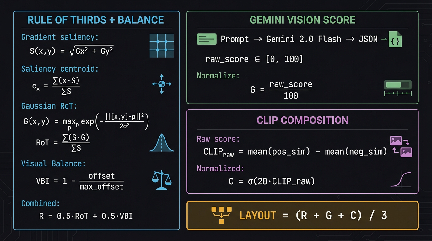
Fig A1. All key equations for the three layout scoring methods.

Method 1: Rule of Thirds + Visual Balance

Gradient saliency:

$$S(x,y) = \text{GaussianBlur}\!\left(\sqrt{G_x^2 + G_y^2}\right)$$

Saliency centroid:

$$c_x = \frac{\sum_{x,y} x \cdot S(x,y)}{\sum_{x,y} S(x,y)}, \quad c_y = \frac{\sum_{x,y} y \cdot S(x,y)}{\sum_{x,y} S(x,y)}$$

Gaussian reward field at power points:

$$G(x,y) = \max_{p \in \{P_1, P_2, P_3, P_4\}} \exp\!\left(-\frac{\|[x,y] – p\|^2}{2\sigma^2}\right), \quad \sigma = W/6$$

Rule-of-thirds score:

$$\text{RoT} = \frac{\sum_{x,y} S(x,y) \cdot G(x,y)}{\sum_{x,y} S(x,y)}$$

Visual Balance Index:

$$\text{VBI} = 1 – \frac{\sqrt{(c_x – W/2)^2 + (c_y – H/2)^2}}{\sqrt{(W/2)^2 + (H/2)^2}}$$

Combined R:

$$R = 0.5 \cdot \text{RoT} + 0.5 \cdot \text{VBI}$$

Method 2: Gemini Vision

$$G = \frac{\text{raw\_score}}{100}, \quad \text{raw\_score} \in [0, 100]$$

Method 3: CLIP Composition

$$\text{CLIP}_{raw} = \frac{1}{22}\sum_{p \in P^+} \cos(e_{img}, e_p) \;-\; \frac{1}{22}\sum_{p \in P^-} \cos(e_{img}, e_p)$$

$$C = \sigma(20 \cdot \text{CLIP}_{raw}) = \frac{1}{1 + e^{-20 \cdot \text{CLIP}_{raw}}}$$

Final combined score

$$\text{Layout} = \frac{R + G + C}{3}$$

---

Appendix B — CLIP Prompt Lists

22 Positive prompts (P⁺)

1. “a well-composed interior photograph with clear focal point”
2. “balanced visual weight distribution across the room”
3. “harmonious furniture arrangement following the rule of thirds”
4. “pleasing spatial depth with distinct foreground and background layers”
5. “symmetrical room layout with balanced proportions”
6. “elegant negative space creating breathing room in the composition”
7. “strong leading lines guiding the eye through the room”
8. “well-framed interior with balanced left and right sides”
9. “layered spatial arrangement with foreground interest and background depth”
10. “centered focal point with supporting elements around it”
11. “dynamic diagonal composition creating visual energy”
12. “open floor plan with clear visual flow and spatial hierarchy”
13. “architectural symmetry with balanced structural elements”
14. “comfortable proportions between furniture and empty space”
15. “visually anchored room with a strong center of gravity”
16. “well-placed focal furniture piece at a rule of thirds intersection”
17. “receding depth perspective creating a sense of spaciousness”
18. “triangular composition formed by three key furniture pieces”
19. “inviting visual pathway from foreground to background”
20. “evenly distributed visual interest across the frame”
21. “grounded composition with heavier elements at the bottom”
22. “clear spatial zones separating functional areas of the room”

22 Negative prompts (P⁻)

1. “cluttered room with no clear focal point or visual hierarchy”
2. “unbalanced composition with everything pushed to one side”
3. “chaotic furniture arrangement with no spatial logic”
4. “flat composition with no depth or layering”
5. “cramped room with furniture blocking all negative space”
6. “awkward framing cutting off furniture and architectural features”
7. “top-heavy composition with visual weight concentrated above”
8. “empty room with no visual anchor or interest”
9. “disorganized layout with competing focal points everywhere”
10. “tunnel vision composition with everything in the center”
11. “random furniture placement with no spatial relationship”
12. “claustrophobic framing with no breathing room”
13. “lopsided room with asymmetric visual weight”
14. “no sense of depth or spatial dimension”
15. “furniture floating in space with no grounding or context”
16. “visually chaotic room with too many competing elements”
17. “dead center bullseye composition with no visual flow”
18. “obstructed view with foreground blocking the scene”
19. “scattered objects with no compositional structure”
20. “monotonous flat wall with no spatial variation”
21. “poorly staged interior with awkward empty gaps”
22. “overwhelming visual density with no resting points for the eye”

---

dataHacker.rs — Chapter 19: Layout Scoring
Author: Vladimir Matic