LLM_log #012: Introduction to Diffusion Models — From Noise to Geometry to Sampling
Highlights:
In this post we build a complete understanding of diffusion models from the ground up — what they are, how images are represented, how the network is trained, what it geometrically learns, and finally how we turn that geometry into samples using DDIM and DDPM. Every formula is accompanied by concrete numbers you can verify by hand. So let’s begin!
Tutorial Overview:
- What Are Diffusion Models?
- How Images Are Represented
- The Denoiser Network
- Noise Schedules
- The Training Objective
- The Two Moons Toy Model
- What Did the Model Learn? — The Geometry
- The Closed-Form Solution
- The Fundamental Theorem
- Why You Can’t Sample in One Step
- DDIM — The Deterministic Sampler
- Numerical Walkthrough: 5 Steps by Hand
- DDPM — Adding Stochasticity
- DDIM vs DDPM: When to Use Which
- Digression: Is L2 Distance Any Good for Images?
- Summary
1. What Are Diffusion Models?
Diffusion models are a class of generative models inspired by physical diffusion processes — specifically Brownian motion, where particles randomly spread out over time.
The core idea has two phases. The forward process gradually destroys structure in data by adding Gaussian noise step by step, until the data becomes pure noise. The reverse process is what the model learns — starting from noise and iteratively denoising to recover realistic data samples.
Formally, if we denote the clean data as \(\mathbf{x}_0\) and progressively noisier versions as \(\mathbf{x}_1, \mathbf{x}_2, \ldots, \mathbf{x}_T\), the model learns the reverse conditional:
$$p_\theta(\mathbf{x}_{t-1} \mid \mathbf{x}_t)$$
while the forward noising process \(q(\mathbf{x}_t \mid \mathbf{x}_{t-1})\) is fixed and requires no learning.
| Step | What happens | Who does it |
|---|---|---|
| Forward \(q(\mathbf{x}_t \mid \mathbf{x}_{t-1})\) | Add noise | Fixed math, no learning |
| Reverse \(p_\theta(\mathbf{x}_{t-1} \mid \mathbf{x}_t)\) | Remove noise | Neural network |
Why diffusion beats VAEs and GANs:
VAEs learn a lower bound — the objective is approximate, causing blurry outputs. GANs play a min-max game between generator and discriminator — unstable, requires many tricks. Diffusion does simple regression: predict the noise. Stable MSE loss, no adversary.
The price: slow sampling — 100–1000 denoising steps vs. one forward pass in a GAN.
2. How Images Are Represented
A real image pixel is an integer from 0 to 255 (8-bit). For an RGB image of size 256×256:
$$256 \times 256 \times 3 = 196{,}608 \text{ numbers}$$
So \(n = 196{,}608\) and the image lives in \(\mathbb{R}^n\).
Normalization to \([-1, 1]\): diffusion models don’t work directly in \([0, 255]\). Before feeding to the network, pixels are normalized:
$$x = \frac{\text{pixel} – 127.5}{127.5}$$
So pixel \(0 \to -1.0\), pixel \(255 \to +1.0\), pixel \(128 \to \approx 0.0\).
Why normalize? Gaussian noise \(\mathcal{N}(0,1)\) lives naturally around \([-3, +3]\). If your data is in \([0, 255]\) and you add noise of scale \(\sigma = 1\), that’s barely perceptible. The math works cleanly when data and noise live in the same scale.
Concrete example. One pixel = 200 (light gray):
$$x_0 = \frac{200 – 127.5}{127.5} = 0.569$$
Add noise with \(\sigma = 0.5\), \(\epsilon = 1.2\):
$$x_\sigma = 0.569 + 0.5 \times 1.2 = 1.169$$
Note it went above 1.0 — perfectly fine during diffusion. Only at the very end do we clip and denormalize back to \([0, 255]\).
3. The Denoiser Network
The denoiser is a neural network:
$$\epsilon_\theta : \mathbb{R}^n \times \mathbb{R}_+ \to \mathbb{R}^n$$
It takes a noisy image and a noise level, and outputs the predicted noise:
$$\epsilon_\theta(\underbrace{x_0 + \sigma\epsilon}_{\text{noisy image}},\ \underbrace{\sigma}_{\text{noise level}}) = \underbrace{\hat{\epsilon}}_{\text{predicted noise}}$$
| Symbol | Meaning |
|---|---|
| \(\mathbb{R}^n\) | Noisy image — vector of \(n\) pixel values |
| \(\mathbb{R}_+\) | A single positive number: the noise level \(\sigma > 0\) |
| \(\to \mathbb{R}^n\) | Predicted noise, same size as input |
| \(\theta\) | Learned weights and biases, updated by gradient descent |
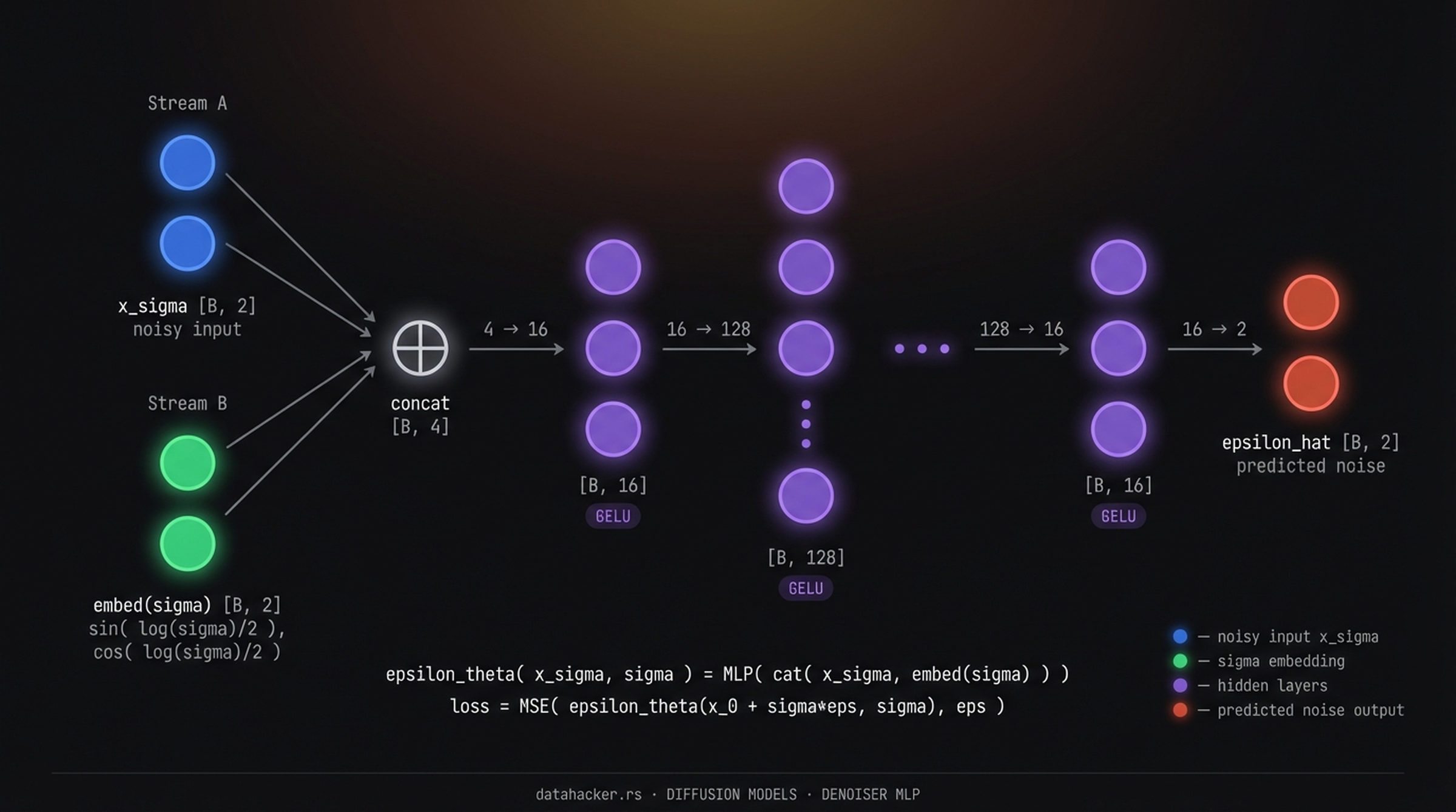
Fig 1. MLP denoiser for Two Moons. Two input streams — noisy point [latex]x_\sigma \in \mathbb{R}^2[/latex] (blue) and sinusoidal sigma embedding (green) — are concatenated to a 4D vector, passed through GELU layers with widths 16→128→16, and projected to [latex]\hat{\epsilon} \in \mathbb{R}^2[/latex] (red).
Why does the network need \(\sigma\) as input? Because the same noisy pixel value means different things at different noise levels. If \(\sigma = 0.01\) there is almost no noise and \(x_0 \approx x_\sigma\). If \(\sigma = 10\) the original \(x_0\) could be anything — the network must know which regime it is in.
4. Noise Schedules
The noise schedule maps a timestep \(t \in [0, 1]\) to a noise level \(\sigma\): \(t = 0\) is low noise (data almost clean), \(t = 1\) is high noise (data is pure noise). In practice noise levels range from \(\sigma_{\min} = 0.01\) to \(\sigma_{\max} = 100\), discretized into 100–1000 steps.
$$t = 1 \to \sigma_1 = 0.01 \quad \text{(barely noisy)}$$
$$t = 500 \to \sigma_{500} = 1.0 \quad \text{(moderately noisy)}$$
$$t = 1000 \to \sigma_{1000} = 100 \quad \text{(pure noise)}$$
Older papers (DDPM) use timestep indices \(t\). Newer papers (EDM) use \(\sigma\) directly — cleaner, because \(\sigma = 1.0\) is immediately meaningful while \(t = 500\) tells you nothing without knowing the schedule.
Why not train on one noise level? Each sample in every training batch gets a different, randomly sampled noise level. This forces the network to generalize across all \(\sigma\) simultaneously — which is exactly what makes the reverse process work across hundreds of steps.
| Schedule | Behavior |
|---|---|
| Cosine | More time at medium noise |
| EDM training | Concentrated around \(\sigma \approx 1\) |
| EDM sampling | More uniform, covers low noise well |
5. The Training Objective
The denoiser network \(\epsilon_\theta\) is trained to minimize the mean squared error between the noise it predicts and the actual noise that was added:
$$L(\theta) := \mathbf{E}_{x_0,\, \sigma,\, \epsilon} \left\| \epsilon_\theta(x_0 + \sigma\epsilon,\ \sigma) – \epsilon \right\|^2$$
| Symbol | What it is |
|---|---|
| \(x_0\) | Clean sample from training data |
| \(\sigma\) | Noise level sampled from the schedule |
| \(\epsilon \sim \mathcal{N}(0, I)\) | Random noise vector |
| \(x_0 + \sigma\epsilon\) | Noisy input fed to the network |
| \(\epsilon_\theta(\cdot)\) | The network’s predicted noise |
| \(\epsilon\) | The actual noise added — the target |
One training step in plain English: ① Pick a clean sample \(x_0\) from training data. ② Sample a random noise level \(\sigma\) from the schedule. ③ Sample random noise \(\epsilon \sim \mathcal{N}(0, I)\). ④ Corrupt the sample: \(x_\sigma = x_0 + \sigma\epsilon\). ⑤ Ask the network to predict \(\epsilon\) from \((x_\sigma, \sigma)\). ⑥ Compute MSE between prediction and truth, backpropagate.
6. The Two Moons Toy Model
To understand diffusion concretely, we train on a 2D dataset — two crescent-shaped point clouds called Two Moons. Instead of \(n = 196{,}608\) pixel dimensions, we have \(n = 2\). Everything else is identical.
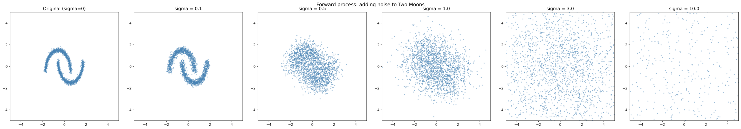
Fig 2. Forward process in action. At [latex]\sigma = 0[/latex] the two crescents are sharp. By [latex]\sigma = 1[/latex] the structure is almost gone. By [latex]\sigma = 10[/latex] the points are pure Gaussian noise.
def get_data(n_samples=2000, noise=0.05):
    X, _ = make_moons(n_samples=n_samples, noise=noise)
    X = (X - X.mean(axis=0)) / X.std(axis=0)  # normalize
    return torch.tensor(X, dtype=torch.float32)
The network for this toy model is a small MLP — 4 inputs (2 for the noisy point, 2 for the sigma embedding), outputs 2 numbers (predicted noise). The sigma embedding uses sinusoidal encoding:
$$\text{embed}(\sigma) = \left[\sin\!\left(\frac{\log\sigma}{2}\right),\ \cos\!\left(\frac{\log\sigma}{2}\right)\right]$$
Raw scalars are poor neural network inputs. Sinusoidal encoding gives smooth, bounded features that change predictably with \(\sigma\).
class Denoiser(nn.Module):
    def __init__(self, hidden_dims=(16, 128, 128, 128, 128, 16)):
        super().__init__()
        dims   = [4] + list(hidden_dims) + [2]
        layers = []
        for in_dim, out_dim in zip(dims[:-1], dims[1:]):
            layers += [nn.Linear(in_dim, out_dim), nn.GELU()]
        layers.pop()  # no activation on output
        self.net = nn.Sequential(*layers)

    def forward(self, x, sigma):
        sigma_emb = get_sigma_embedding(sigma).to(x.device)
        net_input = torch.cat([x, sigma_emb], dim=-1)
        return self.net(net_input)
Training loop:
def train(model, data, epochs=10000, batch_size=512, lr=1e-3,
          sigma_min=0.01, sigma_max=10.0):

    optimizer = torch.optim.Adam(model.parameters(), lr=lr)
    loader    = DataLoader(TensorDataset(data), batch_size=batch_size, shuffle=True)
    sigmas    = get_training_sigmas(sigma_min=sigma_min, sigma_max=sigma_max)

    for epoch in range(epochs):
        for (x0,) in loader:
            sigma   = sigmas[torch.randint(len(sigmas), (x0.shape[0],))]
            eps     = torch.randn_like(x0)
            x_sigma = x0 + sigma.unsqueeze(-1) * eps
            eps_hat = model(x_sigma, sigma)
            loss    = nn.MSELoss()(eps_hat, eps)
            optimizer.zero_grad(); loss.backward(); optimizer.step()
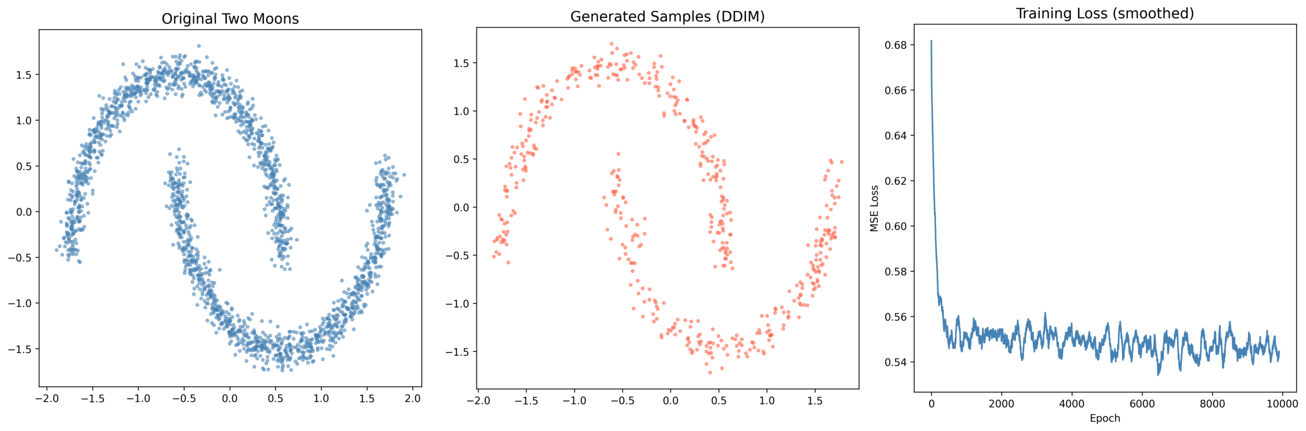
Fig 3. Left: original Two Moons training set. Center: generated samples via DDIM after training. Right: training loss (smoothed). The loss drops sharply in the first 500 epochs then plateaus. Generated samples clearly recover the two crescent shapes from pure noise.
7. What Did the Model Learn? — The Geometry
After training, we visualize what the model learned by plotting the vector field — at every point in 2D space, which direction would the network push a noisy sample?
$$\text{arrow at } x = -\epsilon_\theta(x, \sigma) \cdot \sigma$$
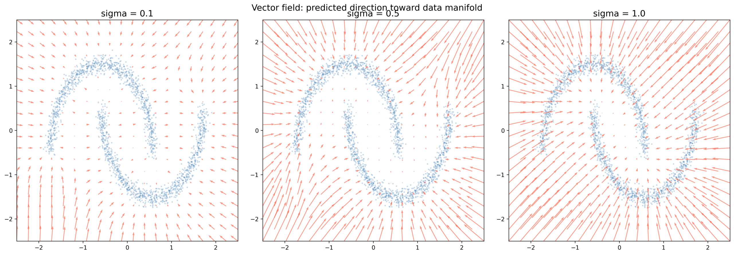
Fig 4. Learned vector field at three noise levels. At [latex]\sigma = 0.1[/latex] (left) arrows point sharply toward the nearest crescent — the model has learned the exact geometry of the data manifold. At [latex]\sigma = 0.5[/latex] (center) the field is smoother, less certain. At [latex]\sigma = 1.0[/latex] (right) arrows point toward the center of mass of the whole dataset — the model averages over all possibilities because at this noise level the data structure is nearly destroyed.
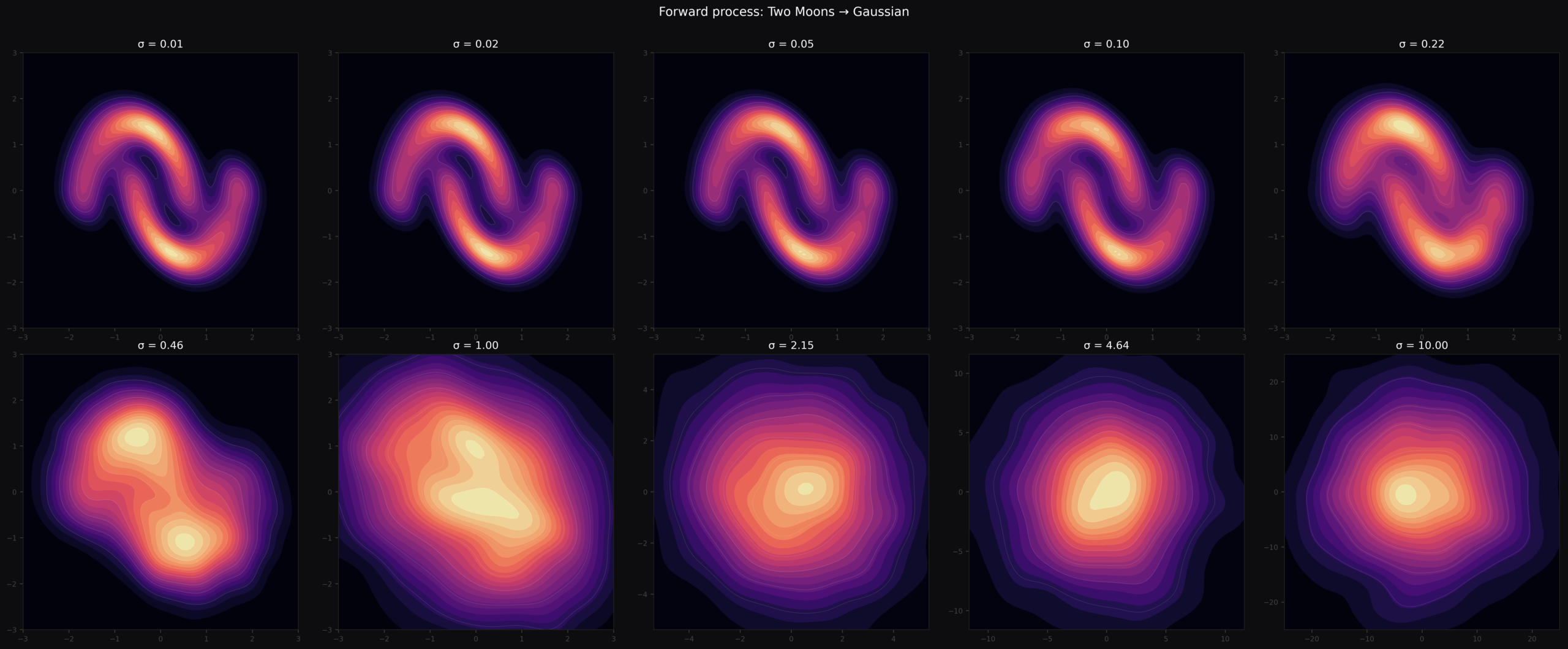
Fig 5. KDE panels across 10 noise levels. The two sharp crescent peaks at [latex]\sigma = 0.01[/latex] slowly merge into a single blob and eventually a centered Gaussian at [latex]\sigma \geq 2[/latex]. The reverse process must undo exactly this — reconstructing two-peaked structure from a featureless Gaussian.
8. The Closed-Form Solution
Here is something remarkable: the ideal denoiser has a closed-form solution. No approximation needed. Given the training dataset \(\mathcal{K}\), the perfect denoiser at any noise level \(\sigma\) is exactly:
$$\epsilon^*(x_\sigma, \sigma) = \frac{\displaystyle\sum_{x_0 \in \mathcal{K}} (x_\sigma – x_0)\, \exp\!\left(-\|x_\sigma – x_0\|^2 / 2\sigma^2\right)}{\displaystyle\sigma \sum_{x_0 \in \mathcal{K}} \exp\!\left(-\|x_\sigma – x_0\|^2 / 2\sigma^2\right)}$$
| Part | What it does |
|---|---|
| \((x_\sigma – x_0)\) | Displacement vector from training point \(x_0\) toward noisy input \(x_\sigma\) |
| \(\exp(-\|x_\sigma – x_0\|^2 / 2\sigma^2)\) | Gaussian weight — closer training points get exponentially more weight |
| Denominator | Normalisation — makes weights sum to 1 |
| \(\sigma\) in denominator | Scales the result to noise units |
At small \(\sigma\) — the Gaussian weights are very sharp. The nearest training point dominates (weight can be 800× larger than the second nearest). The denoiser essentially snaps to the nearest data point: \(\epsilon^* \approx (x_\sigma – x_0^*) / \sigma\) where \(x_0^*\) is the nearest neighbor.
At large \(\sigma\) — all weights become nearly equal. Every training point contributes roughly the same. The denoiser points toward the global centroid of the dataset — the average of all training points. This is why one-step sampling fails: at the starting noise level you are always pointing at the average, which is empty space between clusters.
9. The Fundamental Theorem
The closed-form solution is not just a formula — it reveals the deep geometry of what the network learns.
Define the σ-smoothed distance function from a point \(x\) to the dataset \(\mathcal{K}\):
$$\text{dist}_\mathcal{K}(x, \sigma) = -\sigma^2 \log\!\left(\sum_{x_0 \in \mathcal{K}} \exp\!\left(-\frac{\|x_0 – x\|^2}{2\sigma^2}\right)\right)$$
This is a soft, differentiable version of the distance to the nearest point. At small \(\sigma\) it approximates the hard nearest-neighbor distance. At large \(\sigma\) it sees the entire dataset as one blurry mass.
Theorem: For all \(\sigma > 0\) and \(x \in \mathbb{R}^n\):
$$\frac{1}{2} \nabla_x \, \text{dist}_\mathcal{K}^2(x, \sigma) = \sigma \cdot \epsilon^*(x, \sigma)$$
In plain words: the ideal denoiser is the gradient of the smoothed distance function. When you train a neural network to predict noise via MSE, you are implicitly teaching it the complete multi-scale geometry of the data manifold.
Why this matters. The denoiser does not memorize individual training examples. It learns the geometry — how far every point in space is from the data manifold, at every scale. At \(\sigma = 5\) it knows the rough shape of the data. At \(\sigma = 0.1\) it knows the precise local curvature. The \(\sigma\)-annealing during sampling exploits this multi-scale map: navigate globally first, refine locally last.
10. Why You Can’t Sample in One Step
Given the vector field, why not just take one giant step — start from noise, ask the network where the data is, jump there?
Look again at the closed-form solution at large \(\sigma\). The Gaussian weights \(\exp(-d^2 / 2\sigma^2)\) are nearly flat — every training point gets roughly equal weight. The denoiser predicts the average displacement toward all training points simultaneously. For the Two Moons dataset, that average points at the empty space between the two crescents. Jump there and you land nowhere on the manifold.
Analogy. Imagine finding your seat in a dark stadium. From the entrance (high \(\sigma\)) you can only sense the average direction of the crowd — toward the center. As you walk closer and your eyes adjust (lower \(\sigma\)), you can make out sections, then rows, then your exact seat. One step from the entrance to your seat in the dark is impossible. You need many small steps as the picture gradually sharpens.
Multi-step sampling lets the network use its local geometric knowledge progressively: big coarse steps first, fine corrections last.
11. DDIM — The Deterministic Sampler
DDIM (Denoising Diffusion Implicit Models, Song et al. 2020) is the cleanest modern sampler. The update rule is:
$$x_{t-1} = x_t + (\sigma_{t-1} – \sigma_t)\, \epsilon_\theta(x_t, \sigma_t)$$
At each step: ask the network for the noise direction \(\epsilon_\theta\), then move by that direction scaled by how much \(\sigma\) drops. Note that \((\sigma_{t-1} – \sigma_t)\) is negative because \(\sigma\) is decreasing — so we step opposite to the predicted noise, toward the predicted clean data.
@torch.no_grad()
def ddim_sample(model, n_samples=500, n_steps=200,
                sigma_min=0.01, sigma_max=10.0):

    # Geometric (log-spaced) sigma schedule: large to small
    sigmas = torch.exp(
        torch.linspace(np.log(sigma_max), np.log(sigma_min), n_steps)
    )

    x = torch.randn(n_samples, 2) * sigma_max  # start from pure noise

    for i in range(len(sigmas) - 1):
        sigma_t      = sigmas[i].expand(n_samples)
        sigma_t_prev = sigmas[i + 1].expand(n_samples)
        eps_hat      = model(x, sigma_t)
        x            = x + (sigma_t_prev - sigma_t).unsqueeze(-1) * eps_hat

    return x.numpy()
Why log-spaced \(\sigma\)? Linear spacing wastes steps. At \(\sigma = 10\) vs \(\sigma = 9\) the geometry barely changes — a big step is fine. At \(\sigma = 0.2\) vs \(\sigma = 0.1\) the geometry changes dramatically — fine steps matter. Geometric spacing allocates more steps where they help most: the low-\(\sigma\) regime. This is why DDIM produces good results in 20–50 steps instead of 1000.
Deterministic. Same starting noise \(z\) → same final sample every time. The trajectory is fully determined by \(z\) — enabling reproducibility and image interpolation.
Invertible. Run the update backwards to encode a real image into noise, manipulate it, then decode back. This is the basis for image editing in diffusion models.
Straight trajectories. The deterministic update integrates the learned vector field like Euler’s method — the paths are nearly straight lines.
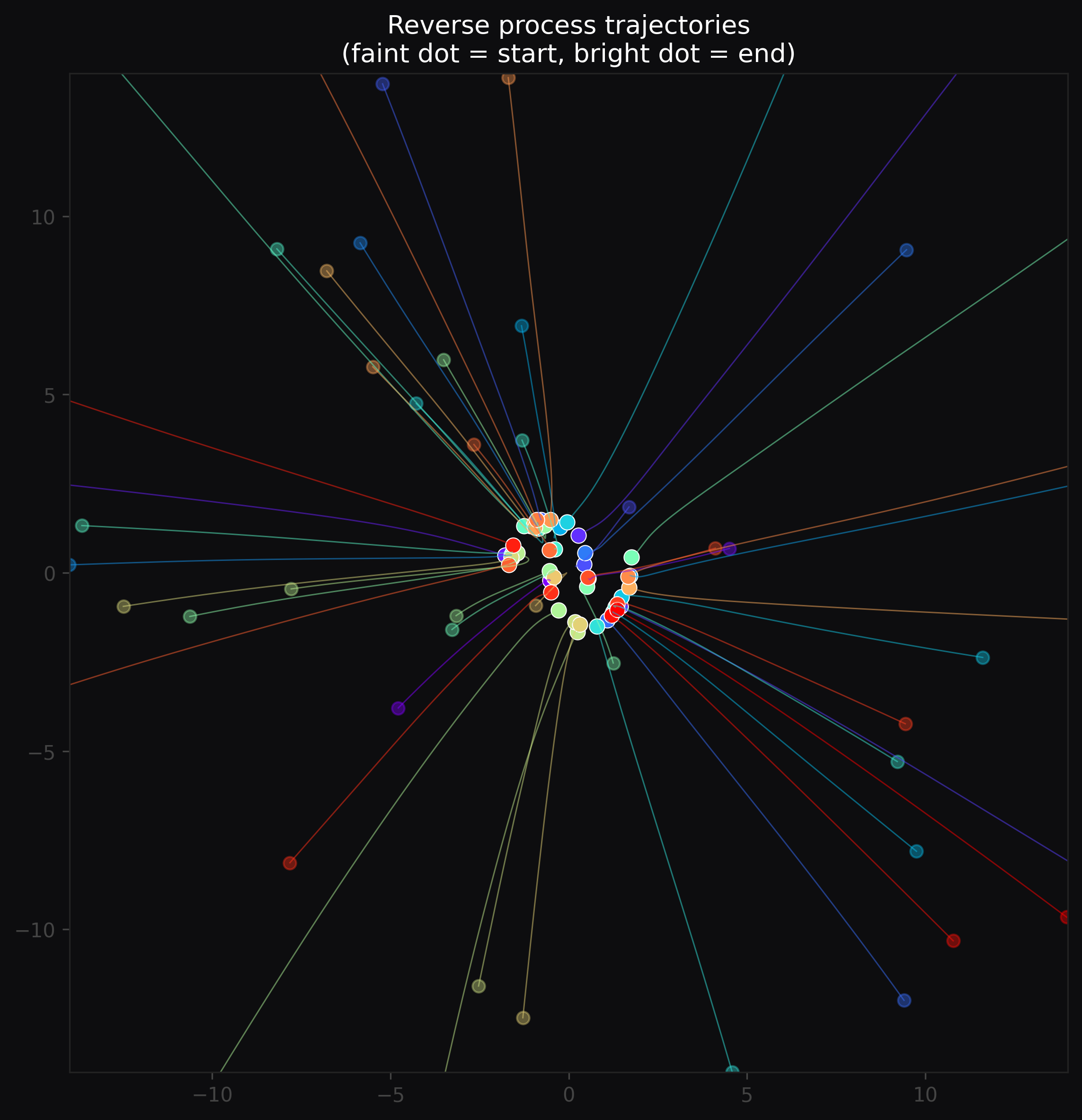
Fig 6. Reverse process trajectories. Faint dots = starting positions (pure noise), bright dots = final positions (on the data manifold). Each colored path traces one particle’s journey from high [latex]\sigma[/latex] to low [latex]\sigma[/latex] — nearly straight lines, converging onto both crescents.
12. Numerical Walkthrough: 5 Steps by Hand
Let’s trace a single point through DDIM concretely — five steps, real numbers.
Setup: \(\sigma\) schedule (log-spaced): 10.0 → 4.6 → 2.2 → 1.0 → 0.46 → 0.01. Starting point: \(x_T = (6.2,\ -4.1)\) from \(\mathcal{N}(0, 10^2 I)\). Update rule: \(x_{t-1} = x_t + (\sigma_{t-1} – \sigma_t) \cdot \epsilon_\theta(x_t, \sigma_t)\)
| Step | \(x_t\) | \(\sigma_t\) | \(\epsilon_\theta\) | \(\Delta\sigma\) | \(x_{t-1}\) |
|---|---|---|---|---|---|
| 0 | (6.2, −4.1) | 10.0 | (0.62, −0.41) | −5.4 | (2.85, −1.88) |
| 1 | (2.9, −1.9) | 4.6 | (0.54, −0.34) | −2.4 | (1.60, −1.08) |
| 2 | (1.6, −1.1) | 2.2 | (0.75, −0.48) | −1.2 | (0.70, −0.52) |
| 3 | (0.7, −0.5) | 1.0 | (0.88, −0.30) | −0.54 | (0.22, −0.34) |
| 4 | (0.2, −0.3) | 0.46 | (0.95, −0.10) | −0.45 | (−0.23, −0.26) |
Final: \(x_0 \approx (-0.23,\ -0.26)\) — on the left crescent. ✓
Steps 0 and 1 make large jumps — coarse navigation at high \(\sigma\), pointing roughly toward the data. Steps 3 and 4 are tiny precision corrections — fine tuning at low \(\sigma\) where the geometry is sharp. Every step does exactly the right amount of work for its \(\sigma\) level.
13. DDPM — Adding Stochasticity
Ho et al. (2020) introduced a variant that injects fresh noise at each step:
$$x_{t-1} = x_t + (\sigma_{t’} – \sigma_t)\, \epsilon_\theta(x_t, \sigma_t) + \eta\, w_t$$
| Symbol | Meaning |
|---|---|
| \(w_t \sim \mathcal{N}(0, I)\) | Fresh Gaussian noise injected at each step |
| \(\eta = \sqrt{\sigma_{t-1}^2 – \sigma_{t’}^2}\) | Scale of noise injection |
| \(\sigma_{t’}\) | Intermediate sigma, set as \(\mu \cdot \sigma_{t-1}\) where \(\mu \in [0,1)\) controls stochasticity |
| \(\mu = 0\) | Noise term vanishes → collapses to DDIM (deterministic) |
| \(\mu \to 1\) | Full Langevin dynamics — maximum stochasticity |
The same starting noise \(z\) now produces different final samples on different runs — the trajectories wander and explore, finding diverse landing points on the manifold.
Why inject noise at all?
The network \(\epsilon_\theta\) is an approximation of the ideal \(\epsilon^*\). Every step accumulates a small prediction error. In DDIM those errors compound deterministically — a tiny bias at step 1 propagates unchanged through all 200 steps.
The stochastic noise in DDPM acts as a regularizer: it disrupts systematic bias accumulation, preventing trajectories from locking into bad attractors caused by compounding errors. It is the same reason SGD generalizes better than full-batch gradient descent — noise helps escape poor local solutions.
The cost: DDPM typically requires 100–1000 steps vs DDIM’s 20–50.
14. DDIM vs DDPM: When to Use Which
| DDIM | DDPM | |
|---|---|---|
| Same noise → same image | ✓ reproducible | ✗ different each time |
| Trajectory shape | Near-straight | Curved, exploratory |
| Steps needed | 20–50 | 100–1000 |
| Image interpolation | ✓ smooth | ✗ noisy |
| Sample diversity | Lower | Higher |
| Invertible | ✓ | ✗ |
| Used in production | Stable Diffusion (default) | Research, diversity tasks |
Practical rule of thumb: Start with DDIM — faster, reproducible, good enough for most tasks. Switch to a hybrid or full DDPM if you need output diversity, or if DDIM produces mode-collapsed results. You can dial stochasticity continuously: at \(\mu = 0.3\) you get mostly deterministic behavior with mild exploration; at \(\mu = 0.8\) you get rich diversity at the cost of more steps.
15. Digression: Is L2 Distance Any Good for Images?
The entire mathematical framework of diffusion uses the L2 norm between images:
$$\|x_\sigma – x_0\|^2 = \sum_{i=1}^{n} (x_{\sigma,i} – x_{0,i})^2$$
Pixel by pixel, square the difference, sum everything. For a 256×256 RGB image that is 196,608 terms. Is L2 a sensible distance between images? The answer is mostly no — not perceptually.
Take a sharp portrait. Shift it 2 pixels right — L2 distance is enormous, nearly every pixel changed. A human cannot perceive the difference. Now blur the same portrait gently — L2 distance is small. A human immediately notices the quality loss. L2 says the blurred image is closer to the original. Human perception says the opposite.
Why diffusion still works despite this: Multi-scale \(\sigma\) training partially compensates. At large \(\sigma\), L2 differences between semantically different images are large and meaningful — a dog and a chair really are far apart at this scale. At small \(\sigma\), nearby L2 neighbors really do look similar — you are comparing almost-identical images differing by tiny noise. The annealing schedule decomposes the learning problem by scale: coarse semantics at large \(\sigma\), fine texture at small \(\sigma\). L2 is adequate at both extremes.
The practical fix: latent diffusion. Stable Diffusion and DALL·E 2 do not work in pixel space. They compress images through a VAE encoder into a latent space — typically \(\mathbb{R}^{4 \times 32 \times 32} \approx \mathbb{R}^{4096}\). The VAE is trained to make L2 distances in latent space perceptually meaningful: nearby latents decode to images that look similar to humans. This is why latent diffusion produces sharper, more detailed results than pixel-space diffusion at the same parameter count.
16. Summary
Let’s close with the full arc.
What we train (sections 1–6): given noisy observation \(x_\sigma = x_0 + \sigma\epsilon\), train a neural network to predict the noise \(\epsilon\) via MSE. Simple, stable, no adversary.
What the network learns (sections 7–9): the gradient of a \(\sigma\)-smoothed distance function to the data manifold \(\mathcal{K}\). The fundamental theorem:
$$\frac{1}{2} \nabla_x \, \text{dist}_\mathcal{K}^2(x, \sigma) = \sigma \cdot \epsilon^*(x, \sigma)$$
By minimizing MSE on noise prediction, the network implicitly learns the complete multi-scale geometry of the data — how far every point in space is from the training data, at every level of resolution from \(\sigma_{\max}\) to \(\sigma_{\min}\).
How we use it (sections 10–14): integrate the learned vector field from high \(\sigma\) to low \(\sigma\) using the DDIM update rule. The closed-form solution shows the denoiser computes a Gaussian-weighted average over training points — exact at small \(\sigma\) (snaps to nearest neighbor), blurry at large \(\sigma\) (global centroid). The \(\sigma\)-annealing schedule traverses this spectrum with every sample: coarse global navigation first, fine local precision last.
The denoiser formula, the L2 geometry, the annealing schedule — each layer is simpler than it first appears, and each connects to something you likely already knew. Take care! 🙂
Reference: MIT 6.S183 IAP 2026 — A Practical Introduction to Diffusion Models.