LLM_log #008: CLIP — Understanding Multimodal AI Through Step-by-Step Experiments
- Transformers for Vision
- Multimodal Embedding Models
- CLIP: Connecting Text and Images
- Hands-On: CLIP Experiments with OpenCLIP
- Can AI See Wealth? Testing CLIP on Real House Prices
- Experiment 6: Text Prompt Scoring
- Experiment 7: Data-Driven Centroids
- Experiment 8: SVM vs Centroid
- Experiment 9: How Much Data Do You Need?
- Key Takeaways
1. Transformers for Vision
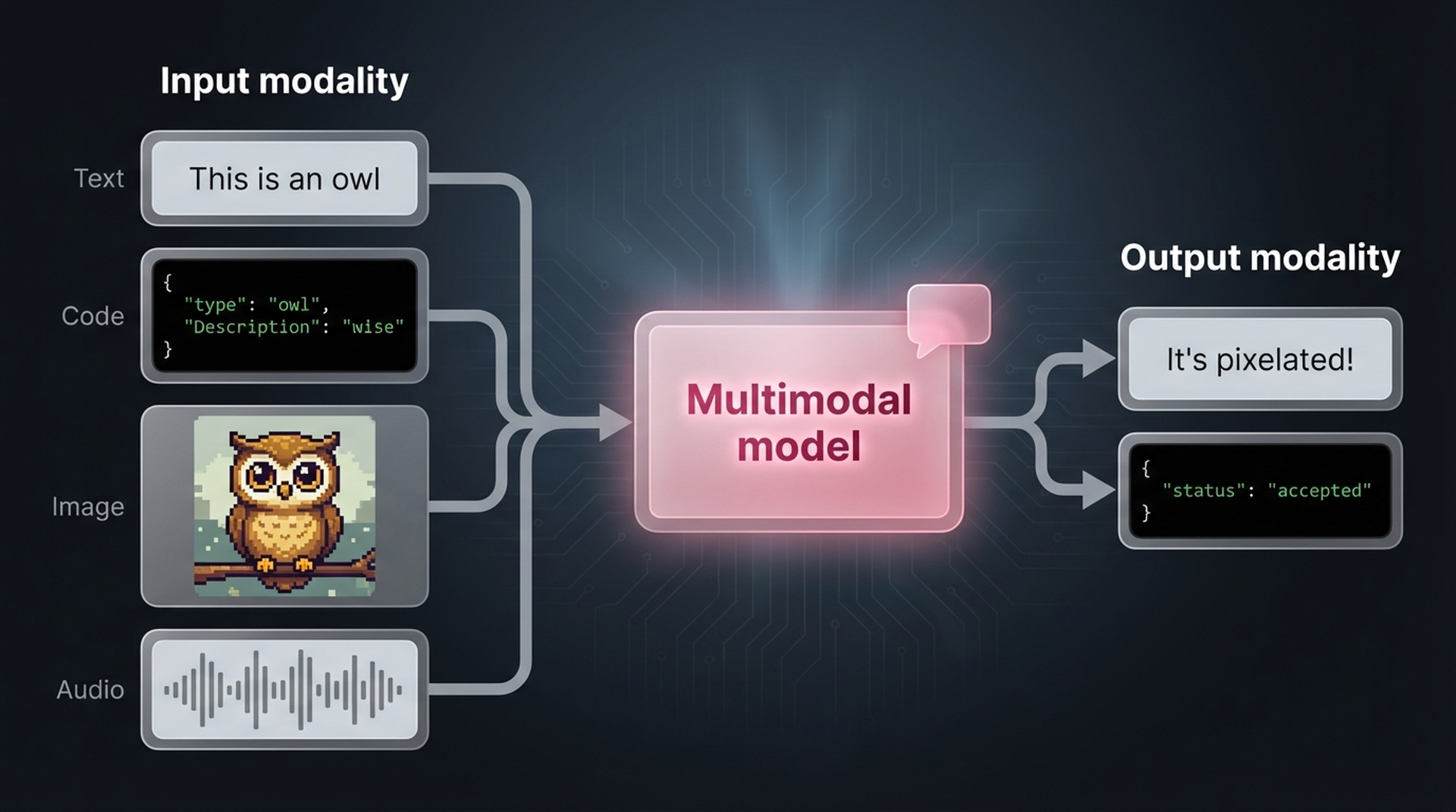
When you think about large language models, multimodality might not be the first thing that comes to mind. After all, they are language models! But models become significantly more useful when they can handle data types beyond text. Imagine a language model that can glance at an image and answer questions about it — that’s where multimodal models come in.
A model that handles both text and images (each of which is called a modality) is said to be multimodal.
In practice, language doesn’t live in a vacuum. Your body language, facial expressions, and intonation all enhance the spoken word. The same applies to AI models — if we enable them to reason about multimodal information, their capabilities increase dramatically, and we can deploy them to solve entirely new categories of problems.
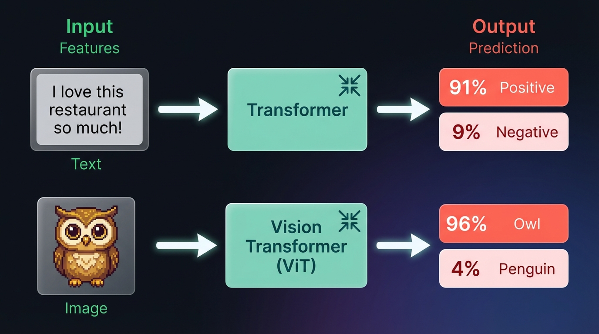
Throughout the deep learning revolution, Transformer-based models have dominated language tasks — from classification and clustering to search and generation. So it’s no surprise that researchers asked: can we bring this success to computer vision?
The answer is the Vision Transformer (ViT), which has shown remarkable performance on image recognition tasks compared to convolutional neural networks (CNNs). Like the original Transformer, ViT transforms unstructured data — in this case an image — into rich representations usable for downstream tasks like classification.
How the Encoder Processes Text
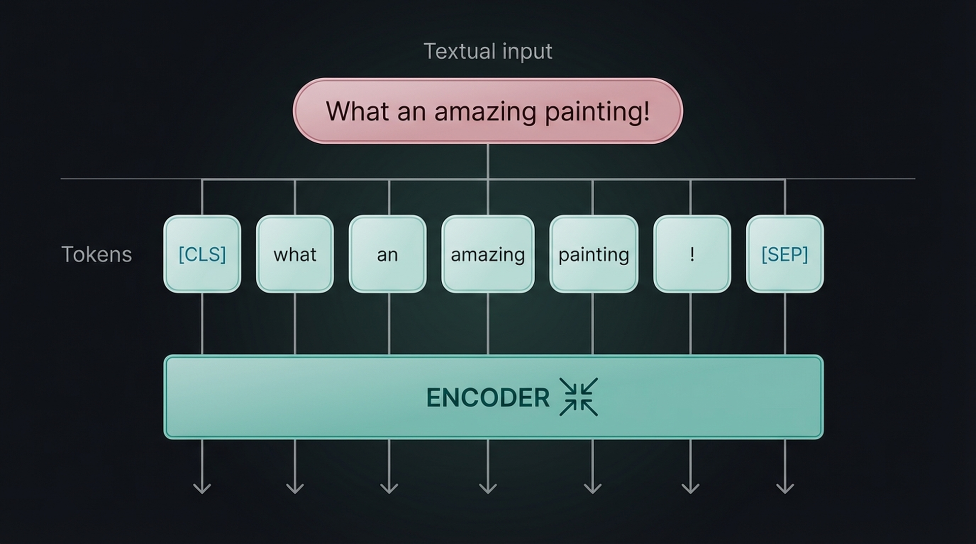
The ViT relies on a core component of the Transformer architecture: the encoder. In text models, the encoder converts tokenized text into numerical representations. Before the encoder can work, though, the text needs to be broken into tokens first.
From Pixels to Patches: Image “Tokenization”
Since images don’t consist of words, the standard text tokenization process can’t be used for visual data. The ViT authors came up with a clever workaround: tokenize images into “words” by splitting them into patches.
Think of it this way — a single pixel conveys almost no information. But when you combine patches of pixels, meaningful visual features start to emerge. ViT exploits this by cutting the image into a grid of sub-images, both horizontally and vertically.
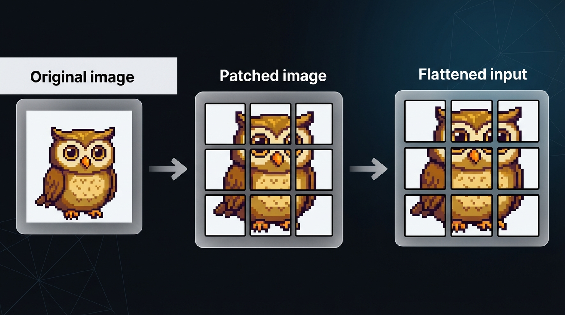
Just like we convert text into tokens, we convert an image into patches. The flattened input of image patches can be thought of as tokens in a sentence. However, unlike text tokens, we can’t just assign each patch an ID — these patches will rarely appear identically in other images, unlike vocabulary words.
Instead, the patches are linearly projected to create numerical representations (embeddings). These embeddings can then be fed into the Transformer encoder, treating image patches the same way as text tokens. A special [CLASS] token is prepended, mirroring the [CLS] token in text models.
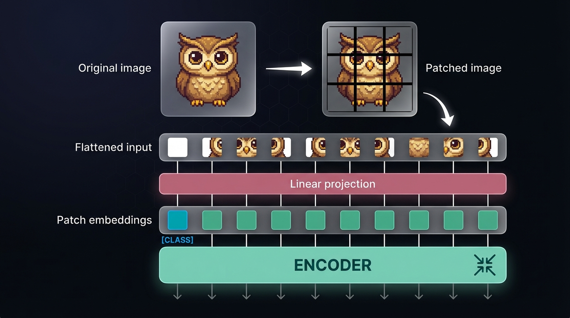
The original ViT paper used 16×16 patches — hence its title “An Image Is Worth 16×16 Words.” What’s fascinating about this approach is that once the embeddings hit the encoder, there’s no difference in how text or images are processed. This architectural elegance is exactly why ViT has become the backbone for making language models multimodal.
2. Multimodal Embedding Models
In earlier work on NLP, embedding models captured the semantic content of text — enabling document search, classification, and clustering. Embeddings are an efficient method for capturing large-scale information and finding the needle in the haystack.
But what if embedding models could capture both text and images in the same vector space? That’s exactly what multimodal embedding models do.
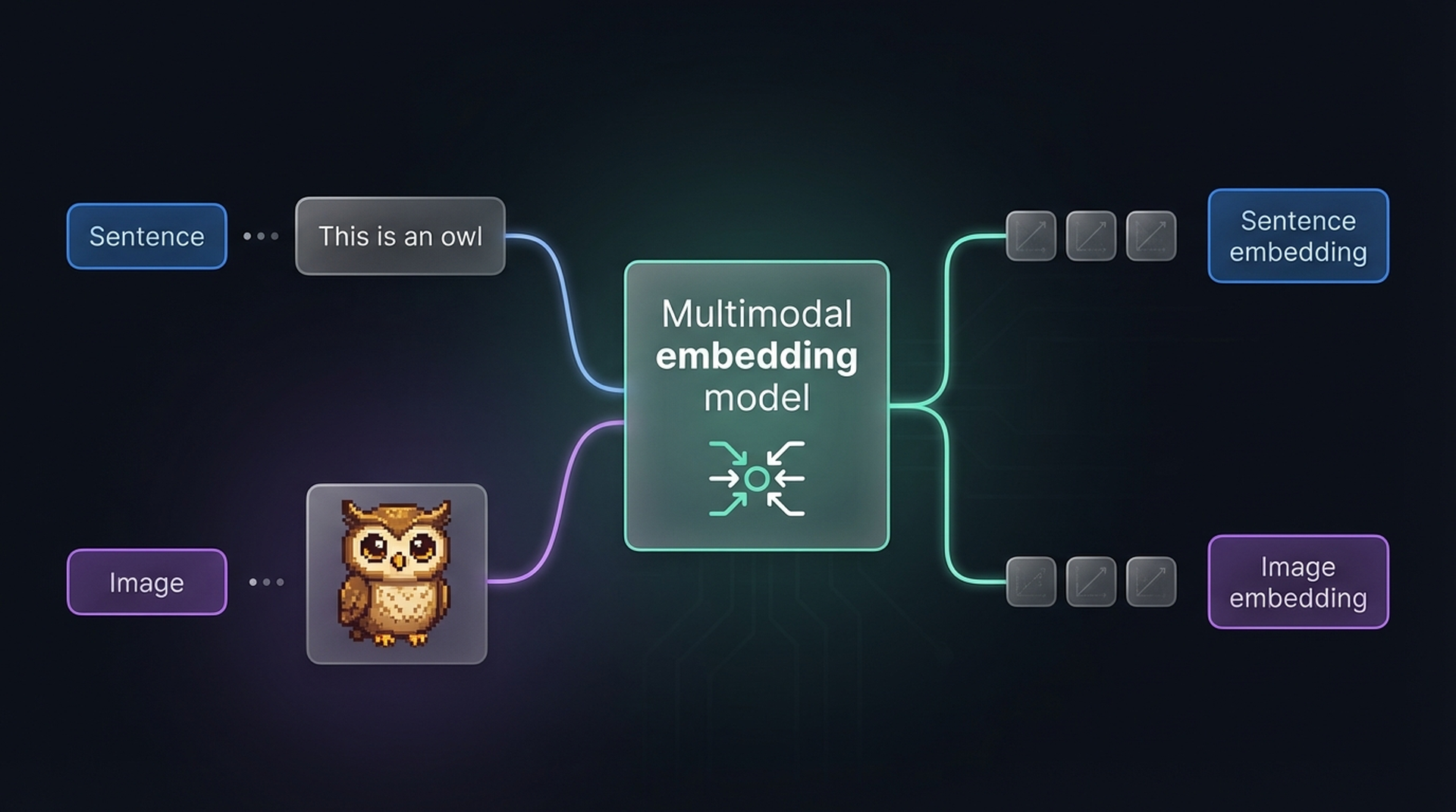
The key advantage: since embeddings from different modalities live in the same space, we can directly compare them. Want to find images that match the description “pictures of a puppy”? Just embed the text, embed the images, and compute their similarity. The reverse works too — find which documents relate to a given image.
3. CLIP: Connecting Text and Images
CLIP (Contrastive Language-Image Pre-training) is the most well-known multimodal embedding model. It computes embeddings for both images and text, placing them in the same vector space so they can be directly compared.
This comparison capability unlocks several powerful tasks:
- Zero-shot classification — compare an image embedding with class description embeddings to find the best match, without any task-specific training
- Clustering — group images and keywords together to discover which descriptions belong to which visual clusters
- Search — across billions of texts or images, quickly find what relates to an input query
- Generation — use multimodal embeddings to drive image generation (e.g., Stable Diffusion)
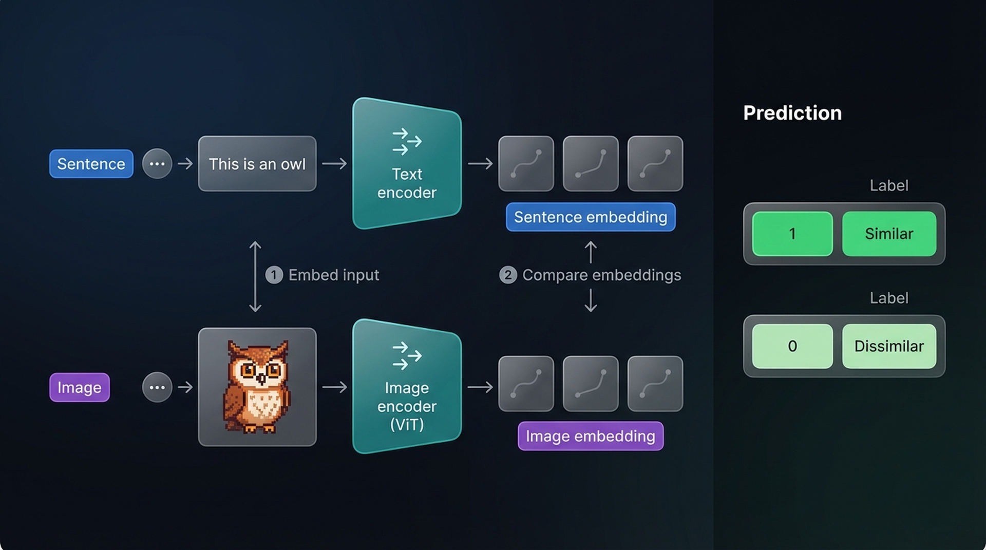
How CLIP Is Trained
The training procedure is surprisingly straightforward. Start with a dataset of millions of image-caption pairs. For each pair, CLIP uses two encoders:
- A text encoder to embed the caption
- An image encoder (ViT) to embed the image
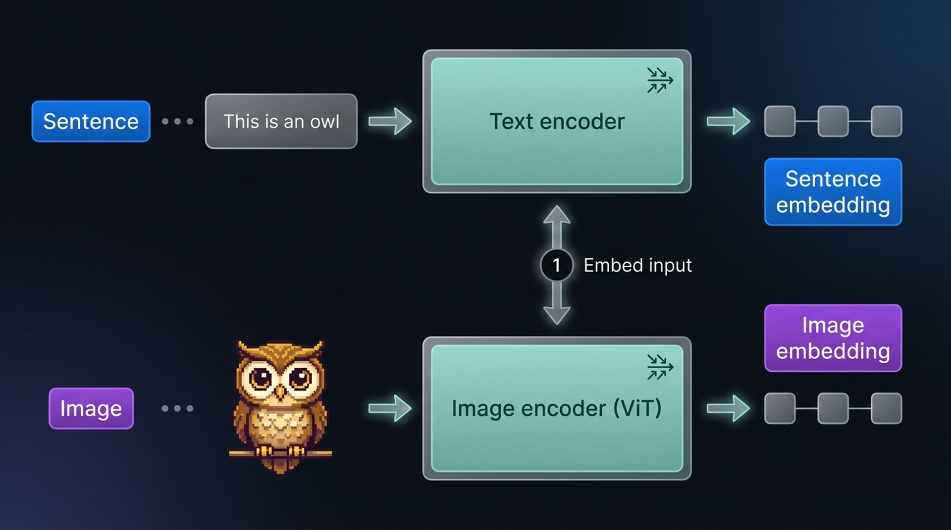
The resulting embeddings are compared via cosine similarity. At the start of training, the similarity between paired image and text embeddings is low since the encoders aren’t yet optimized to share a vector space.
During training, the model optimizes for:
- Maximizing similarity between matching image-caption pairs
- Minimizing similarity between mismatched pairs
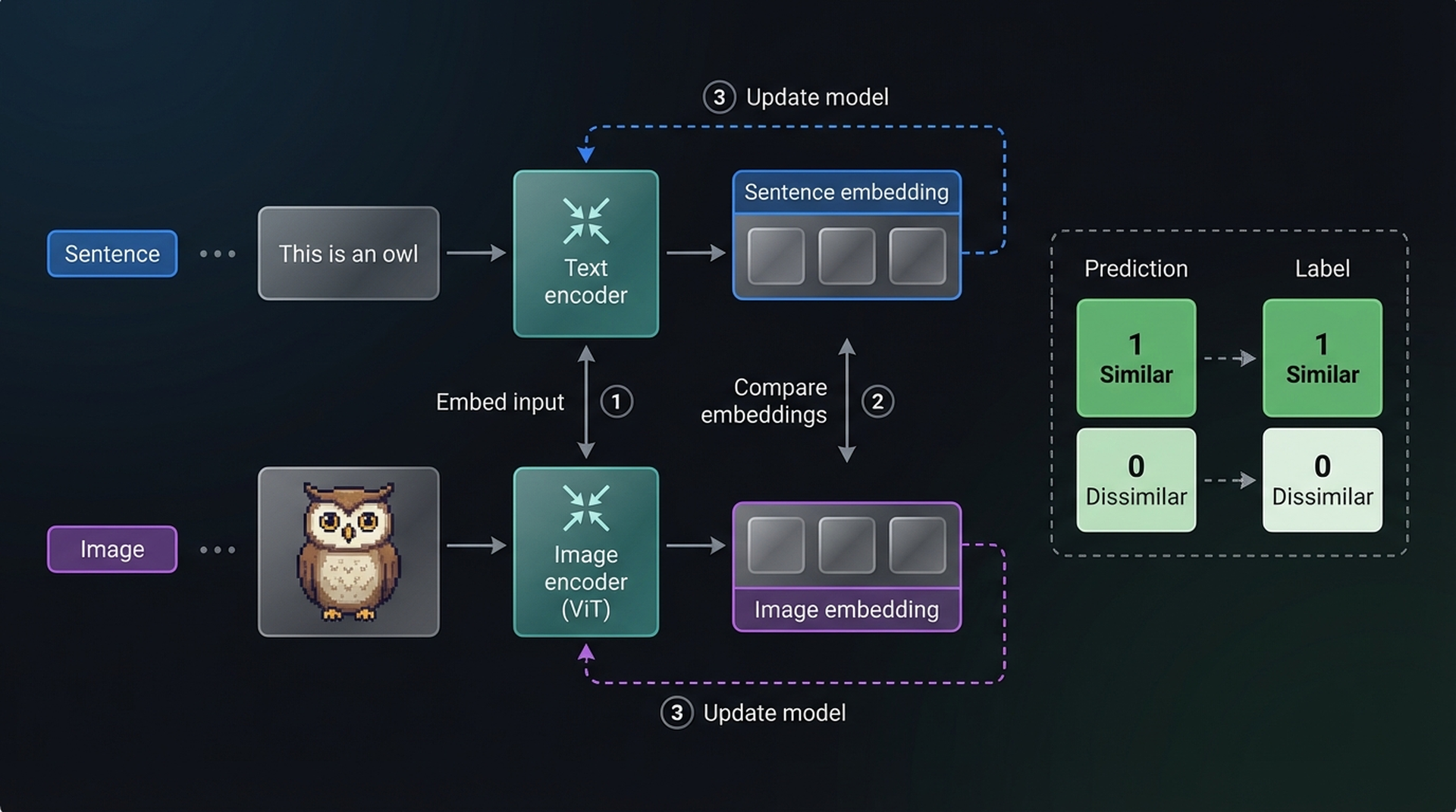
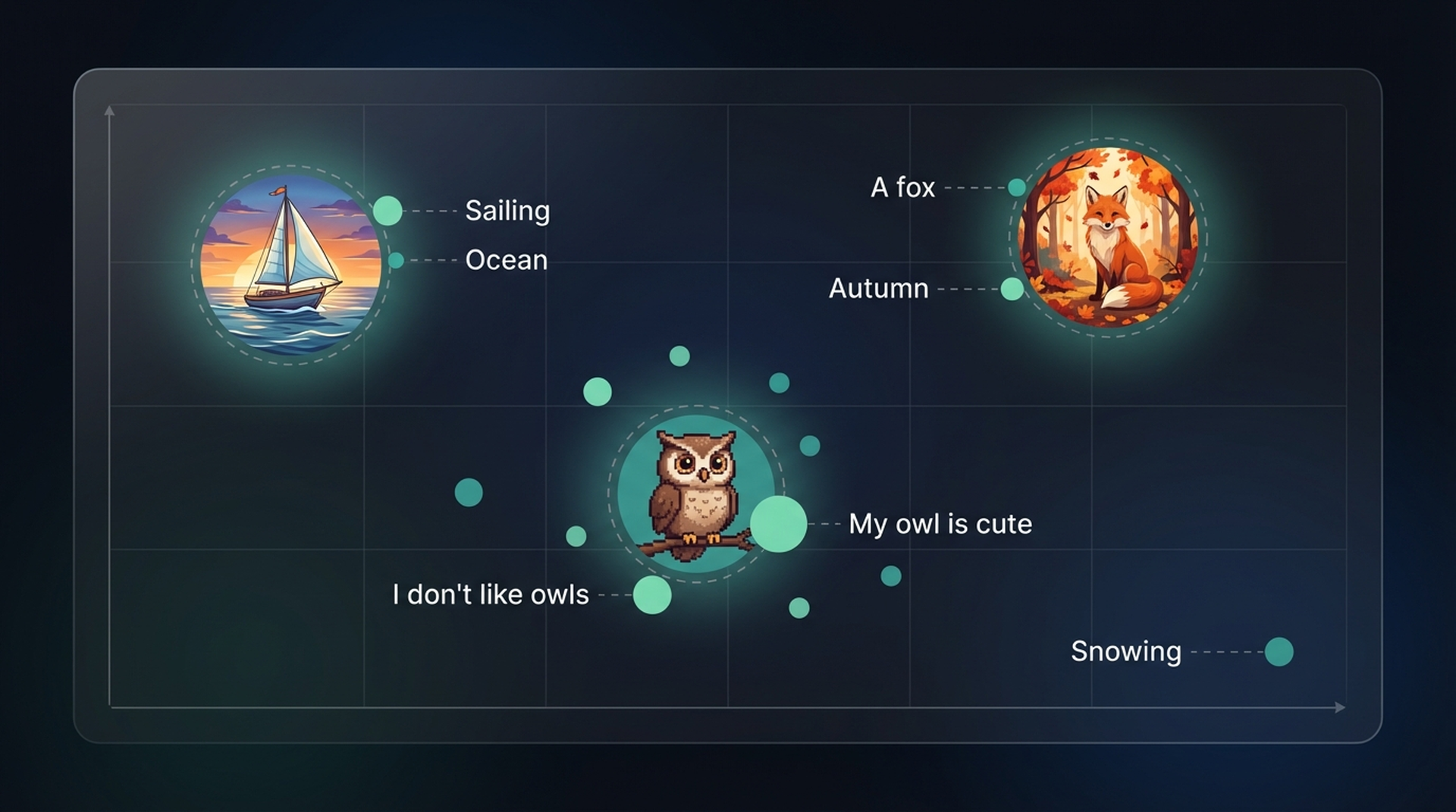
After calculating similarity, both encoders are updated and the process repeats with new batches. This is called contrastive learning — the model learns not just what makes things similar, but crucially what makes them different.
Eventually, the embedding of an owl image should be close to the embedding of “a pixelated image of a cute owl,” while being far from “a sailboat on the ocean.”
4. Hands-On: CLIP Experiments with OpenCLIP
Let’s get our hands dirty. We’ll use OpenCLIP through the transformers library to run real experiments and build intuition for how CLIP behaves.
Setup
import torch
import numpy as np
from PIL import Image
from urllib.request import urlopen
from transformers import CLIPTokenizerFast, CLIPProcessor, CLIPModel

model_id = "openai/clip-vit-base-patch32"

# Load tokenizer, processor, and model
clip_tokenizer = CLIPTokenizerFast.from_pretrained(model_id)
clip_processor = CLIPProcessor.from_pretrained(model_id)
model = CLIPModel.from_pretrained(model_id)
We have three components:
- Tokenizer — handles text input (splitting into tokens)
- Processor — handles image input (resizing, normalization)
- Model — produces embeddings for both modalities
Experiment 1: Embedding a Single Image-Caption Pair
Let’s start with a classic example — a Wikipedia image of an owl:
# Load an image of an owl from Wikipedia
owl_url = "https://upload.wikimedia.org/wikipedia/commons/thumb/2/23/Bubo_virginianus_06.jpg/800px-Bubo_virginianus_06.jpg"
image = Image.open(urlopen(owl_url)).convert("RGB")
caption = "a great horned owl"
First, let’s see how the tokenizer handles our caption:
# Tokenize the caption
inputs = clip_tokenizer(caption, return_tensors="pt")
print(inputs)
# {'input_ids': tensor([[49406, ..., 49407]]), 'attention_mask': tensor([[1, 1, ...]])}

# Convert IDs back to tokens
tokens = clip_tokenizer.convert_ids_to_tokens(inputs["input_ids"][0])
print(tokens)
# ['<|startoftext|>', 'a</w>', 'great</w>', 'horned</w>', 'owl</w>', '<|endoftext|>']
Notice the special start-of-text and end-of-text tokens that bracket the input. Now let’s create the text embedding:
# Create text embedding
text_embedding = model.get_text_features(**inputs)
print(text_embedding.shape)
# torch.Size([1, 512])
A 512-dimensional vector representing our caption. Now the image:
# Preprocess image
processed_image = clip_processor(
    text=None, images=image, return_tensors="pt"
)["pixel_values"]
print(processed_image.shape)
# torch.Size([1, 3, 224, 224])
The processor resized our image to 224×224 pixels — that’s CLIP’s expected input size. Now we embed it:
# Create image embedding
image_embedding = model.get_image_features(processed_image)
print(image_embedding.shape)
# torch.Size([1, 512])
Same shape as the text embedding — 512 dimensions. This is the key insight: both modalities produce vectors in the same space, making them directly comparable.
Computing Similarity
# Normalize embeddings
text_embedding = text_embedding / text_embedding.norm(dim=-1, keepdim=True)
image_embedding = image_embedding / image_embedding.norm(dim=-1, keepdim=True)

# Calculate cosine similarity
text_np = text_embedding.detach().cpu().numpy()
image_np = image_embedding.detach().cpu().numpy()
score = np.dot(text_np, image_np.T)
print(f"Similarity: {score[0][0]:.4f}")
A single similarity score is hard to interpret in isolation. Is 0.30 high? Low? We need a comparison.
Experiment 2: Multi-Image, Multi-Caption Similarity Matrix
This is where CLIP really shines. Let’s load three different images and three captions, then compute the full similarity matrix:
# Load three different images
owl_url = "https://upload.wikimedia.org/wikipedia/commons/thumb/2/23/Bubo_virginianus_06.jpg/800px-Bubo_virginianus_06.jpg"
fox_url = "https://upload.wikimedia.org/wikipedia/commons/thumb/1/1f/Vulpes_vulpes_laying_in_snow.jpg/1280px-Vulpes_vulpes_laying_in_snow.jpg"
sailboat_url = "https://upload.wikimedia.org/wikipedia/commons/thumb/a/a1/Sailboat_in_the_sunset.jpg/1280px-Sailboat_in_the_sunset.jpg"

images = [
    Image.open(urlopen(owl_url)).convert("RGB"),
    Image.open(urlopen(fox_url)).convert("RGB"),
    Image.open(urlopen(sailboat_url)).convert("RGB"),
]

captions = [
    "a photo of an owl",
    "a fox in the snow",
    "a sailboat at sunset",
]

# Embed all images
image_inputs = clip_processor(text=None, images=images, return_tensors="pt")
image_embeddings = model.get_image_features(**image_inputs)

# Embed all captions
text_inputs = clip_tokenizer(captions, padding=True, return_tensors="pt")
text_embeddings = model.get_text_features(**text_inputs)

# Normalize
image_embeddings = image_embeddings / image_embeddings.norm(dim=-1, keepdim=True)
text_embeddings = text_embeddings / text_embeddings.norm(dim=-1, keepdim=True)

# Compute similarity matrix
similarity = (text_embeddings.detach().cpu().numpy()
              @ image_embeddings.detach().cpu().numpy().T)

# Display
import pandas as pd
df = pd.DataFrame(
    similarity,
    index=captions,
    columns=["Owl", "Fox", "Sailboat"]
)
print(df.round(2))
You should see something like this:
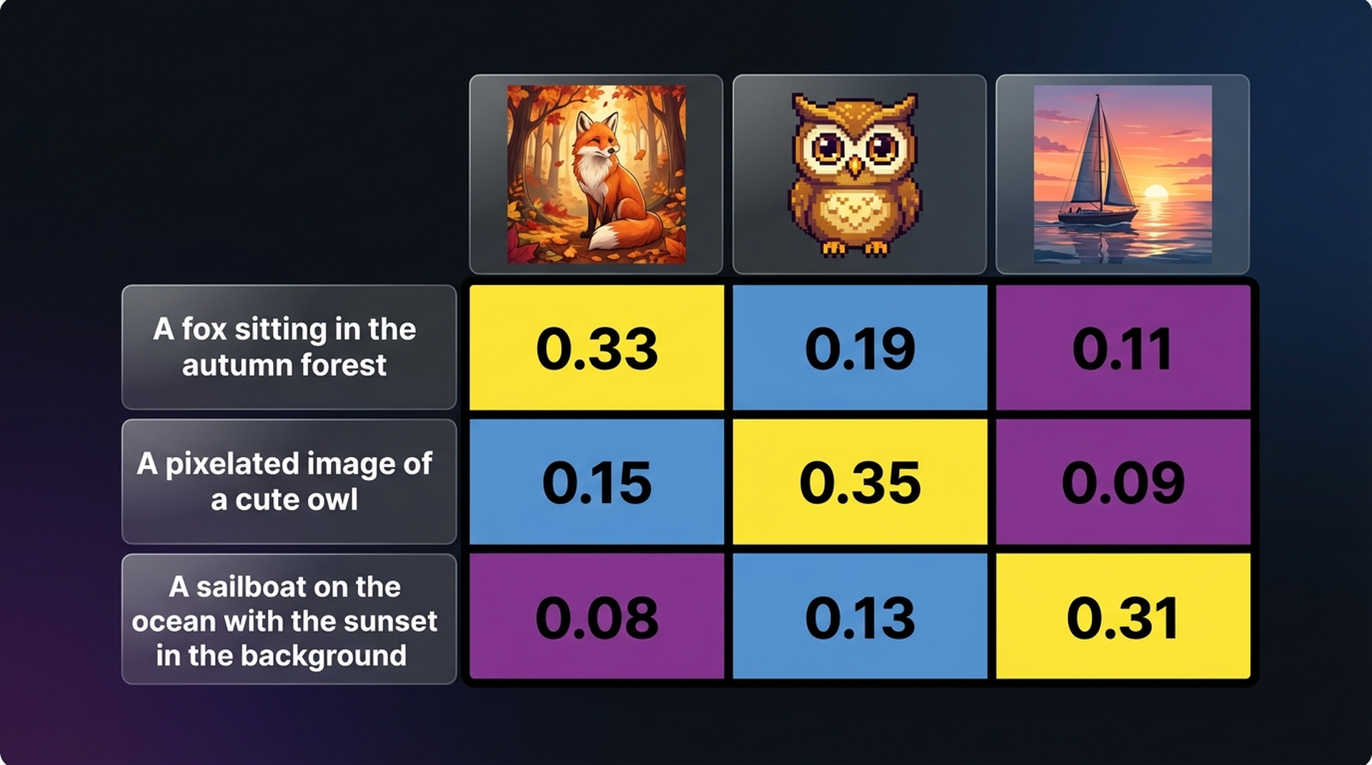
The diagonal dominates — each caption scores highest with its matching image. This is exactly what contrastive learning produces.
Experiment 3: Zero-Shot Image Classification
One of CLIP’s most powerful capabilities is classifying images without any task-specific training. We just embed candidate labels and find the best match:
# Load a test image
test_image = Image.open(urlopen(owl_url)).convert("RGB")

# Define candidate labels
labels = [
    "a photo of an owl",
    "a photo of a dog",
    "a photo of a car",
    "a photo of a mountain",
    "a photo of a flower",
]

# Embed the image
img_input = clip_processor(text=None, images=test_image, return_tensors="pt")
img_emb = model.get_image_features(**img_input)
img_emb = img_emb / img_emb.norm(dim=-1, keepdim=True)

# Embed all labels
txt_input = clip_tokenizer(labels, padding=True, return_tensors="pt")
txt_emb = model.get_text_features(**txt_input)
txt_emb = txt_emb / txt_emb.norm(dim=-1, keepdim=True)

# Compute similarities and convert to probabilities
similarities = (img_emb.detach().cpu().numpy()
                @ txt_emb.detach().cpu().numpy().T)[0]

# Softmax for probabilities
exp_sim = np.exp(similarities * 100)  # temperature scaling
probs = exp_sim / exp_sim.sum()

for label, prob in sorted(zip(labels, probs), key=lambda x: -x[1]):
    print(f"  {label}: {prob:.1%}")
CLIP will confidently assign the highest probability to “a photo of an owl” — despite never being explicitly trained on this classification task. This is the power of learning a shared embedding space.
Experiment 4: Semantic Search with CLIP
Let’s flip the script — instead of classifying an image, let’s search for the best image given a text query:
# We already have embeddings for our three images (owl, fox, sailboat)
# Let's search with a new query
query = "a bird sitting on a branch at night"

query_input = clip_tokenizer(query, return_tensors="pt")
query_emb = model.get_text_features(**query_input)
query_emb = query_emb / query_emb.norm(dim=-1, keepdim=True)

# Compute similarities against all images
sims = (query_emb.detach().cpu().numpy()
        @ image_embeddings.detach().cpu().numpy().T)[0]

image_names = ["Owl", "Fox", "Sailboat"]
for name, sim in sorted(zip(image_names, sims), key=lambda x: -x[1]):
    print(f"  {name}: {sim:.4f}")
Even though none of our captions mentioned “bird” or “branch” or “night,” CLIP’s semantic understanding will rank the owl image highest — it understands that an owl is a bird and is associated with nighttime.
Experiment 5: The Easy Way — sentence-transformers
If you want to skip the manual embedding pipeline, sentence-transformers provides a much cleaner interface for CLIP:
from sentence_transformers import SentenceTransformer, util

# Load CLIP through sentence-transformers
st_model = SentenceTransformer("clip-ViT-B-32")

# Encode images and text with the same API
image_embeddings = st_model.encode(images)
text_embeddings = st_model.encode(captions)

# Compute similarity matrix in one line
sim_matrix = util.cos_sim(image_embeddings, text_embeddings)
print(sim_matrix)
Same results, much less boilerplate. This is the recommended approach for production use.
5. Can AI See Wealth? Testing CLIP on Real House Prices
The experiments above showed that CLIP can match owls to owl descriptions and sailboats to sailing captions. But here’s the question that kept nagging: can CLIP perceive subjective visual qualities? Not just “this is an owl” but “this looks expensive” or “this feels luxurious.” In other words, does CLIP’s embedding space encode the kind of visual judgment that humans make instinctively when scrolling through real estate listings?
To find out, we need ground truth. We need images where we know the price — so we can test whether CLIP’s perception of “premium” correlates with actual market value.
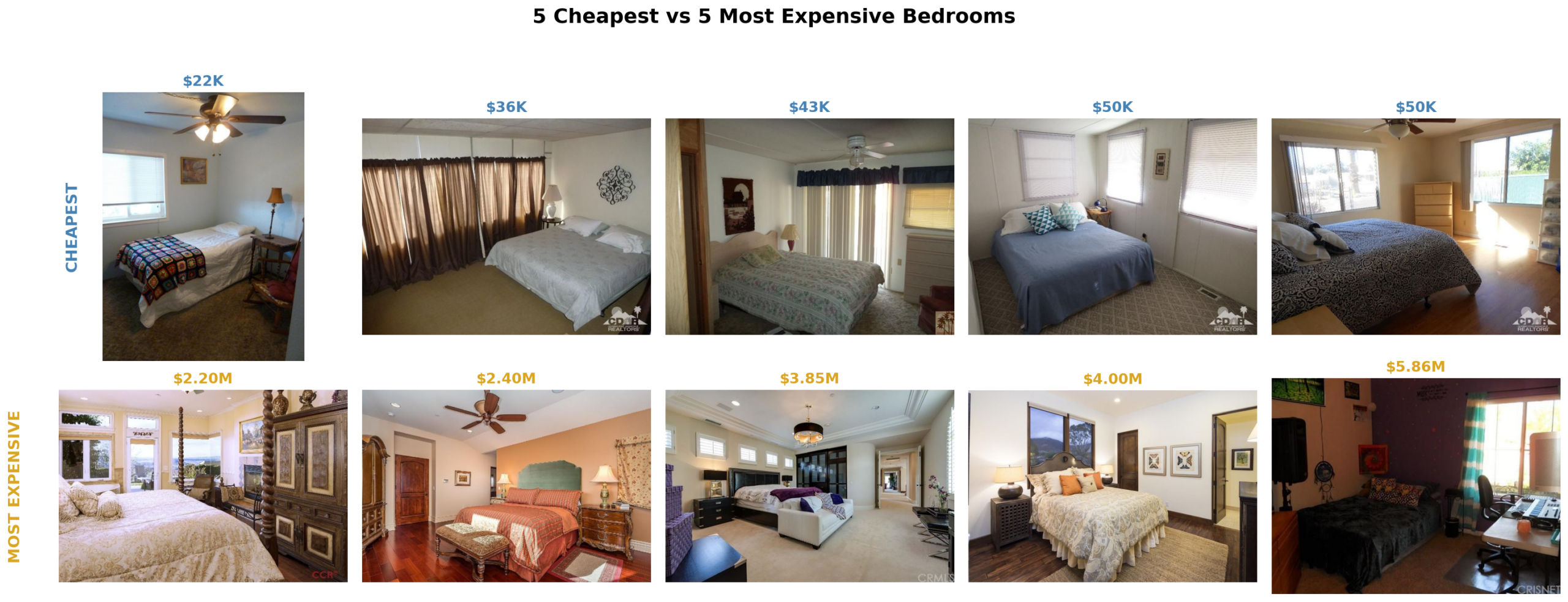
The Dataset: 535 Houses with Real Prices
We use the Houses Dataset by Ahmed & Moustafa (2016) — a benchmark dataset containing 535 houses from California with bedroom, bathroom, kitchen, and frontal photos, plus real sale prices ranging from $22,000 to $5.8 million.
For our experiments, we focus exclusively on bedroom images — interior shots where CLIP’s visual perception of quality matters most. Frontal (exterior) images would confuse the signal since curb appeal and interior quality are different things entirely.
We sort all 535 houses by price and take the 100 cheapest (avg ~$107K) and the 100 most expensive (avg ~$1.3M). The question is simple: when CLIP looks at these bedrooms, can it tell the difference?
Part 2 Setup: Embedding Helpers and Dataset Loading
We reuse the same CLIP model from above. Here are the helper functions that all Part 2 experiments share:
def embed_texts(texts):
    inputs = tokenizer(texts, padding=True, return_tensors="pt").to(device)
    with torch.no_grad():
        text_emb = model.get_text_features(**inputs)
    text_emb /= text_emb.norm(dim=-1, keepdim=True)
    return text_emb.detach().cpu().numpy()

def embed_images(images, bs=32):
    all_emb = []
    for i in range(0, len(images), bs):
        pv = clip_processor(text=None, images=images[i:i+bs],
                            return_tensors="pt")["pixel_values"].to(device)
        with torch.no_grad():
            img_emb = model.get_image_features(pv)
        img_emb /= img_emb.norm(dim=-1, keepdim=True)
        all_emb.append(img_emb.detach().cpu().numpy())
    return np.vstack(all_emb)
And the dataset loading:
# Download Houses Dataset
ZIP_URL = "https://github.com/emanhamed/Houses-dataset/archive/refs/heads/master.zip"
urllib.request.urlretrieve(ZIP_URL, "houses_master.zip")
with zipfile.ZipFile("houses_master.zip", "r") as z:
    z.extractall(".")

# Parse metadata, sort by price
info_path = "Houses-dataset-master/Houses Dataset/HousesInfo.txt"
img_dir = "Houses-dataset-master/Houses Dataset"

meta = []
with open(info_path) as f:
    for i, line in enumerate(f):
        p = line.strip().split()
        if len(p) >= 5:
            meta.append({"id": i+1, "price": float(p[4])})

df = pd.DataFrame(meta).sort_values("price")

def load_bedroom(house_id):
    fp = os.path.join(img_dir, f"{house_id}_bedroom.jpg")
    if os.path.exists(fp):
        try: return Image.open(fp).convert("RGB")
        except: pass
    return None

cheap_ids = df.head(100)["id"].tolist()
expensive_ids = df.tail(100)["id"].tolist()
cheap_imgs = [img for hid in cheap_ids if (img := load_bedroom(hid)) is not None]
exp_imgs = [img for hid in expensive_ids if (img := load_bedroom(hid)) is not None]
6. Experiment 6: Text Prompt Scoring
The most natural approach with CLIP is to use text prompts as measuring sticks. We define what “luxury” and “cheap” mean in words, then measure how close each bedroom image is to each concept. Instead of a single prompt per concept, we use 5 variations for robustness:
lux_prompts = [
    "a luxurious expensive high-end bedroom",
    "a premium elegant sophisticated bedroom interior",
    "a wealthy upscale designer bedroom",
    "a lavish opulent master bedroom suite",
    "a high-class refined luxury bedroom with fine furniture",
]
cheap_prompts = [
    "a cheap budget low-cost bedroom",
    "a basic simple affordable bedroom interior",
    "a poor run-down shabby bedroom",
    "a modest low-budget cramped bedroom",
    "a worn-out old dated bedroom with cheap furniture",
]

# Embed all prompts: (10, 512)
all_prompts_emb = np.vstack([embed_texts(lux_prompts), embed_texts(cheap_prompts)])

# Embed images
cheap_img_emb = embed_images(cheap_imgs)
exp_img_emb = embed_images(exp_imgs)

# Premium score = mean(luxury) - mean(cheap)
cheap_scores = cheap_img_emb @ all_prompts_emb.T
exp_scores = exp_img_emb @ all_prompts_emb.T
cheap_premium = cheap_scores[:, :5].mean(axis=1) - cheap_scores[:, 5:].mean(axis=1)
exp_premium = exp_scores[:, :5].mean(axis=1) - exp_scores[:, 5:].mean(axis=1)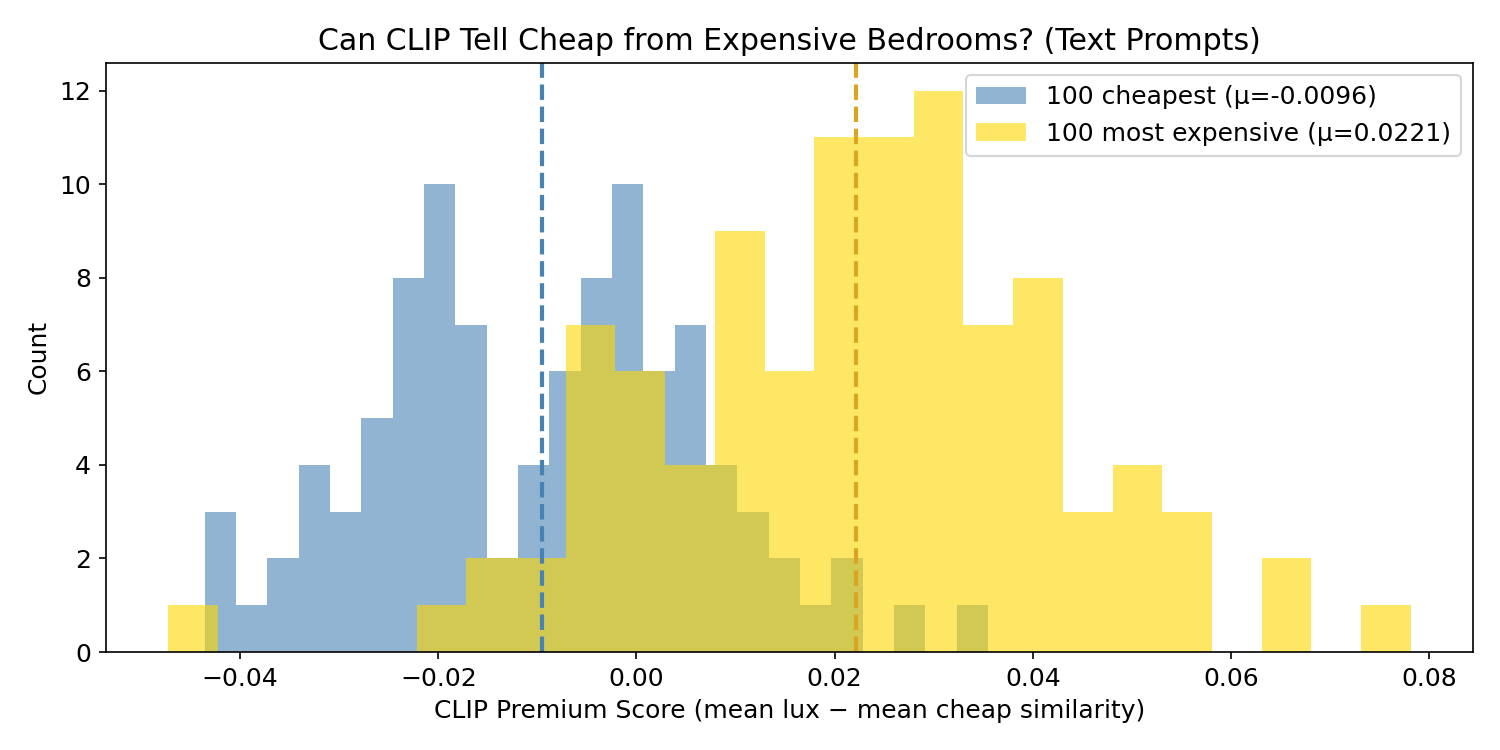
The distributions overlap heavily. The means are separated by only ~0.03 — barely distinguishable. CLIP sees something, but the text prompt approach produces a weak, noisy signal. Many cheap bedrooms score as “premium” and vice versa.
Why? CLIP’s idea of “luxurious” comes from internet image-caption pairs. The word “luxurious” in web captions might describe hotel rooms, magazine shoots, or staged real estate photos — not necessarily what a $1.3M California bedroom actually looks like. There’s a mismatch between CLIP’s learned text-image associations and the visual reality of price brackets.
7. Experiment 7: Data-Driven Centroids
Instead of telling CLIP what luxury looks like with words, what if we show it examples and let the data define the direction?
The idea is simple: compute the mean embedding (centroid) for each class from training data, then define a “luxury axis” as the direction from the cheap centroid to the expensive centroid.
# Split: 80 train, 20 test per group
cheap_train, cheap_test = cheap_img_emb[:80], cheap_img_emb[80:]
exp_train, exp_test = exp_img_emb[:80], exp_img_emb[80:]

# Compute centroids from training data
centroid_cheap = cheap_train.mean(axis=0)
centroid_exp = exp_train.mean(axis=0)

# Define the luxury axis: unit vector from cheap → expensive
luxury_axis = centroid_exp - centroid_cheap
luxury_axis /= np.linalg.norm(luxury_axis)

# Project test images onto this axis
cheap_proj = cheap_test @ luxury_axis
exp_proj = exp_test @ luxury_axis

gap = exp_proj.mean() - cheap_proj.mean()
print(f"Centroid gap: {gap:.4f}")  # ~0.25 — 10x larger than text prompts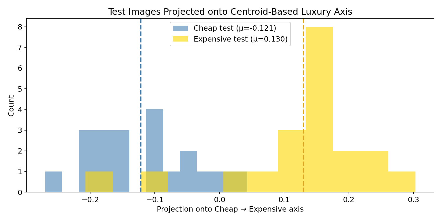
This is dramatically better. The gap between means is ~0.25 — roughly 10x larger than the text prompt approach. The overlap is minimal. CLIP’s embedding space does encode visual luxury — we just needed data-driven directions instead of text prompts to extract it.
The difference comes down to how the “luxury direction” is defined. Text prompts hope that “luxurious expensive high-end bedroom” lands near where real expensive bedrooms live in CLIP’s 512-dim space. But CLIP’s text-trained associations may not align with actual price-correlated visual features. Centroids let the actual bedroom images define the direction — no guessing with words.
Key insight: Prompt engineering has limits. Data-driven directions in embedding space are more powerful than any text prompt you can write.
8. Experiment 8: SVM vs Centroid
The centroid method uses the direction between two class means. But what if the optimal separating direction isn’t the line connecting the means? A Support Vector Machine (SVM) finds the hyperplane that maximizes the margin between classes — potentially a better separator.
We wrapped the centroid method as an sklearn classifier so both approaches could be compared under identical 5-fold cross-validation:
from sklearn.svm import SVC
from sklearn.decomposition import PCA
from sklearn.model_selection import cross_val_score, StratifiedKFold
from sklearn.base import BaseEstimator, ClassifierMixin

class CentroidClassifier(BaseEstimator, ClassifierMixin):
    def fit(self, X, y):
        self.classes_ = np.unique(y)
        self.centroids_ = {c: X[y == c].mean(axis=0) for c in self.classes_}
        self.axis_ = self.centroids_[1] - self.centroids_[0]
        self.axis_ /= np.linalg.norm(self.axis_)
        projs = X @ self.axis_
        self.threshold_ = (projs[y == 0].mean() + projs[y == 1].mean()) / 2
        return self

    def predict(self, X):
        return (X @ self.axis_ >= self.threshold_).astype(int)

# Scale up: 150 cheapest + 150 most expensive bedrooms
X = np.vstack([embed_images(cheap_imgs_150), embed_images(exp_imgs_150)])
y = np.array([0]*len(cheap_imgs_150) + [1]*len(exp_imgs_150))
cv = StratifiedKFold(n_splits=5, shuffle=True, random_state=42)

# Compare across PCA dimensions
dims = [2, 5, 10, 20, 50, 100, 200]
for d in dims:
    X_pca = PCA(n_components=d).fit_transform(X)
    sc_c = cross_val_score(CentroidClassifier(), X_pca, y, cv=cv, scoring="accuracy")
    sc_s = cross_val_score(SVC(kernel="linear", C=1.0), X_pca, y, cv=cv, scoring="accuracy")
    print(f"PCA({d:3d}): Centroid={sc_c.mean():.1%}  SVM={sc_s.mean():.1%}")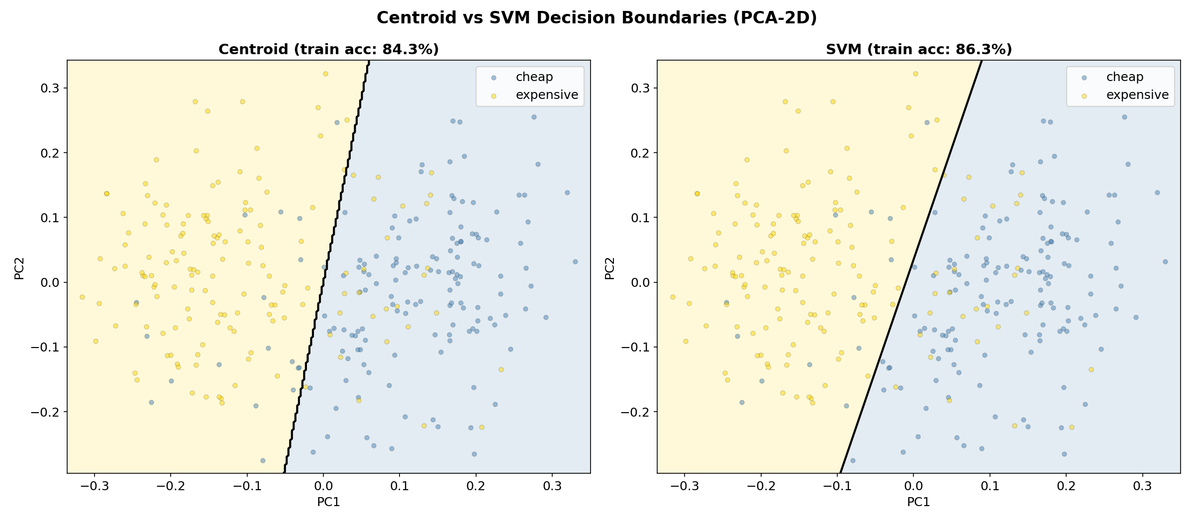
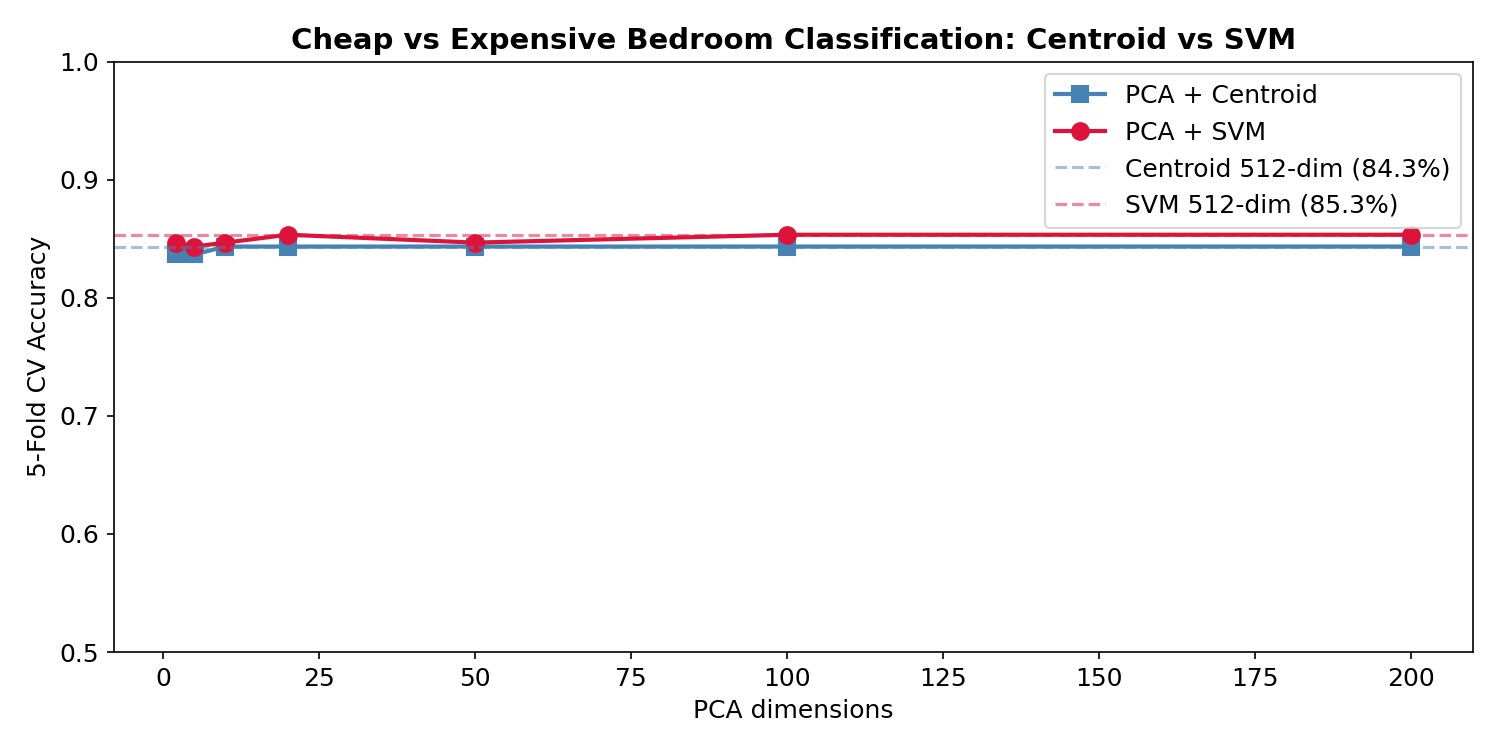
The SVM consistently edges out the centroid by a small margin — it’s optimizing the decision boundary rather than just connecting class means. But the gap is small (~2%), suggesting the class distributions are fairly symmetric in CLIP space.
9. Experiment 9: How Much Data Do You Need?
Perhaps the most practically useful experiment: if you only have a few labeled examples, which approach should you use?
We trained both methods at 10%, 20%, 40%, 60%, 80%, and 100% of the data (300 total samples), averaging over 10 random subsamples. The centroid operates on PCA-10 dimensions (which stabilizes it with few samples), while SVM uses the full 512-dim embeddings.
fractions = [0.1, 0.2, 0.4, 0.6, 0.8, 1.0]
n_repeats = 10
pca_dim = 10

X_pca = PCA(n_components=pca_dim).fit_transform(X)
total = len(X)

for frac in fractions:
    n_use = max(int(total * frac), 10)
    c_accs, s_accs = [], []

    for seed in range(n_repeats):
        rng = np.random.RandomState(seed)
        idx = rng.permutation(total)[:n_use]
        X_sub_pca, X_sub_full = X_pca[idx], X[idx]
        y_sub = y[idx]

        if len(np.unique(y_sub)) < 2: continue
        n_folds = min(5, min(np.bincount(y_sub)))
        cv = StratifiedKFold(n_splits=n_folds, shuffle=True, random_state=seed)

        sc_c = cross_val_score(CentroidClassifier(), X_sub_pca, y_sub, cv=cv, scoring="accuracy")
        sc_s = cross_val_score(SVC(kernel="linear", C=1.0), X_sub_full, y_sub, cv=cv, scoring="accuracy")
        c_accs.append(sc_c.mean())
        s_accs.append(sc_s.mean())

    print(f"{frac*100:5.0f}% ({n_use:3d}): Centroid={np.mean(c_accs):.1%}  SVM={np.mean(s_accs):.1%}")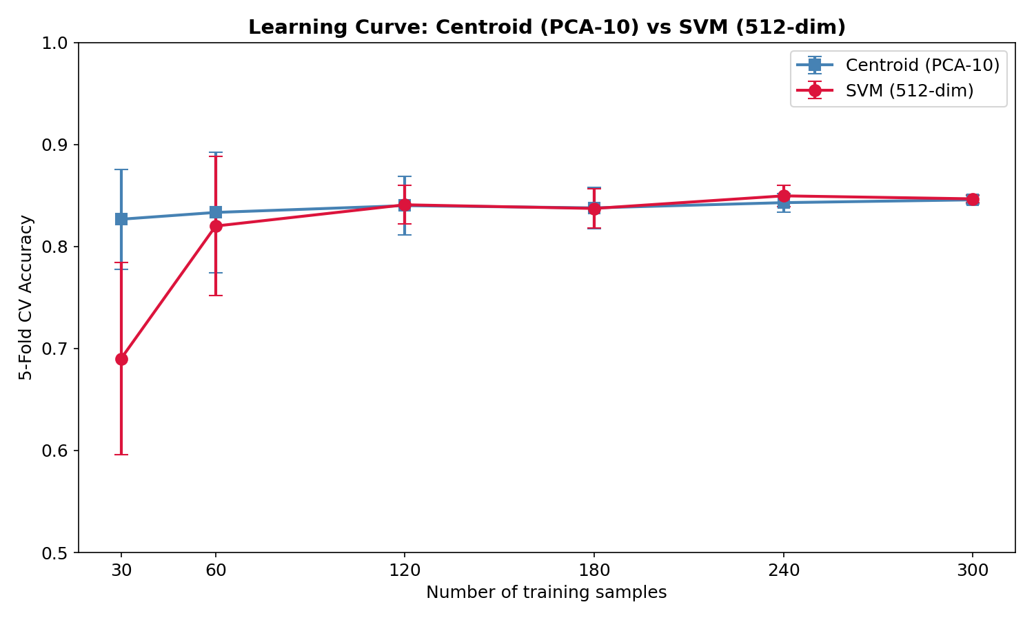
The key finding: at low data (30 samples, ~15 per class), the centroid method outperforms SVM. With only 15 examples per class, computing a mean is more stable than fitting a maximum-margin classifier in 512 dimensions. The SVM catches up around 60–120 samples and they converge at full data.
10. Key Takeaways
| Method | Accuracy | Labeled Data | Key Advantage |
|---|---|---|---|
| Text Prompts | ~55–60% | 0 (zero-shot) | No labeled data at all |
| Centroid | ~83–85% | 15+ per class | Stable at low N, simple |
| SVM | ~84–86% | 50+ per class | Optimal boundary |
Vision Transformers repurpose the text Transformer architecture for images by treating image patches as tokens — a beautifully simple idea that works remarkably well.
Multimodal embedding models place different modalities in the same vector space, enabling direct comparison between text and images.
CLIP learns these shared representations through contrastive learning — maximizing similarity for matching pairs while minimizing it for mismatches. The result is a model that can perform zero-shot classification, semantic search, and clustering across modalities without task-specific training.
For practical applications — brand perception, product quality, aesthetic scoring, design evaluation — the lesson from our house price experiments is clear:
Don’t rely solely on text prompt engineering. Collect a small set of labeled examples (even 20–30 per class), compute centroids in CLIP embedding space, and you’ll get dramatically better results than any prompt you can write. The centroid method is essentially a linear probe on frozen CLIP features — the simplest possible classifier on top of a powerful foundation model. And for most practical applications, it’s all you need.