LLM_log #007: From Random Text to Coherent Language – Pretraining Your First Large Language Model
Highlights: In this guide, you’ll learn how to pretrain a large language model from scratch — implementing training loops, evaluation metrics, and advanced text generation strategies. We’ll build a complete GPT-style training pipeline, watch it evolve from random gibberish to coherent text, and explore techniques like temperature scaling and top-k sampling. By the end, you’ll load professional pretrained weights into your own architecture.
Source: This is part of our ongoing “Building LLMs from Scratch” series on datahacker.rs. All code examples and figures have been adapted from the original concepts to provide a unique learning experience.
Tutorial Overview:
- The Big Picture: Where Pretraining Fits
- Generating Text with an Untrained Model
- Measuring Quality: The Cross-Entropy Loss Pipeline
- Preparing Training Data
- The Training Loop
- Beyond Greedy Decoding: Temperature and Top-k
- Saving, Loading, and Professional Weights
1. The Big Picture: Where Pretraining Fits
Every powerful language model starts life generating complete gibberish. GPT-4, Claude, Gemini — they all began producing random token sequences. Yet through pretraining, these models eventually learn to craft coherent prose and engage in meaningful conversations.
In the previous chapters we implemented a complete GPT-style architecture — data sampling, attention mechanisms, and the full transformer stack. Now it’s time to bring that architecture to life through training.
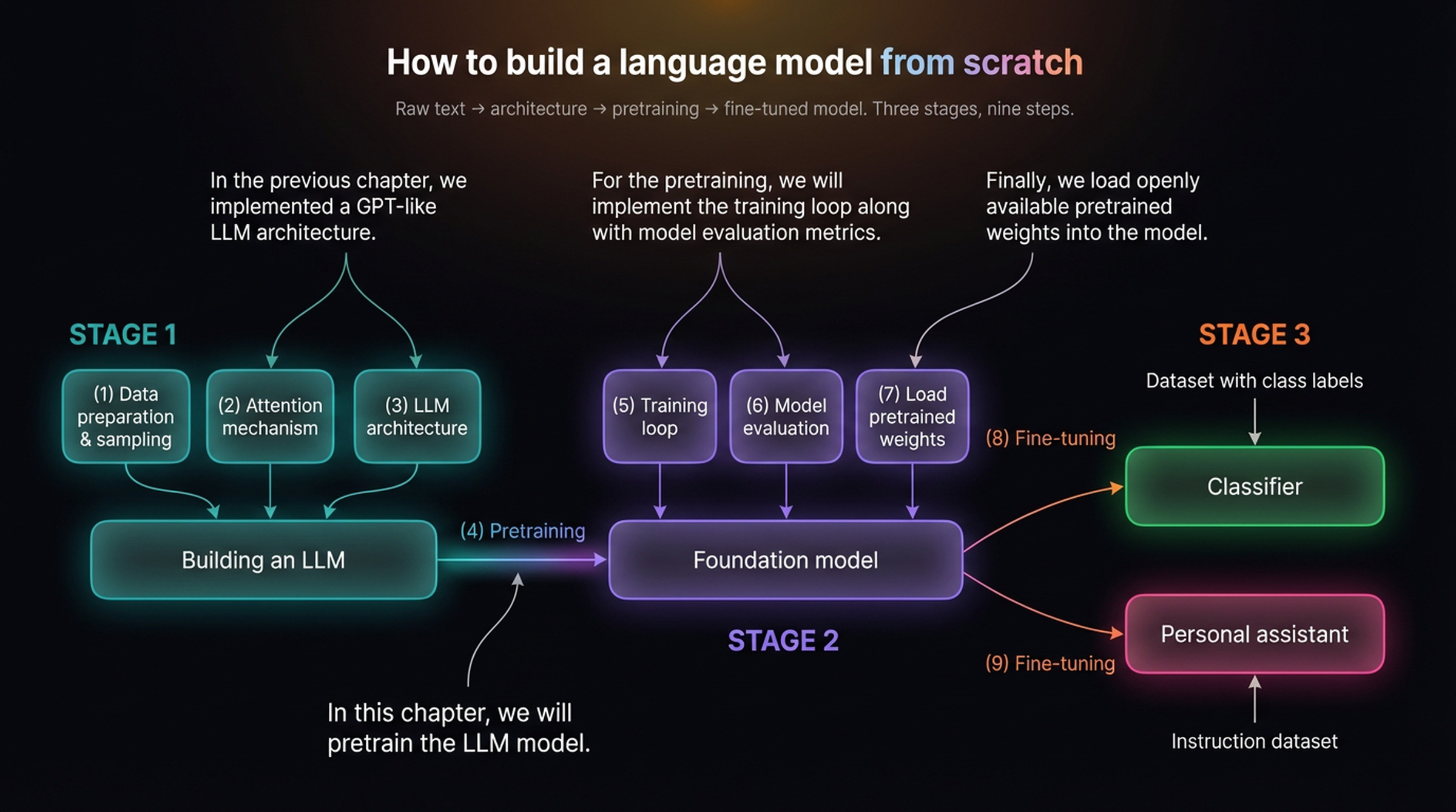
The three-stage journey of building an LLM. Stage 1 (architecture) is complete from previous chapters. This chapter tackles Stage 2: pretraining. Stage 3 (fine-tuning) comes next.
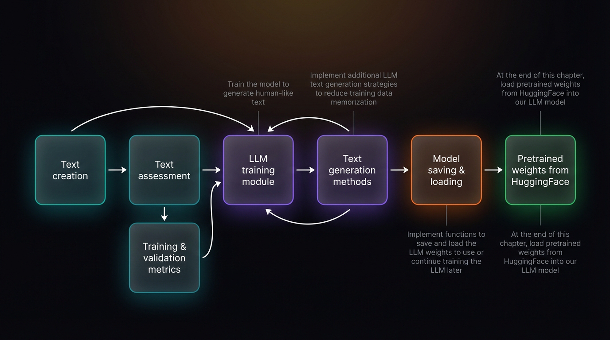
Our chapter roadmap breaks down into seven interconnected steps:
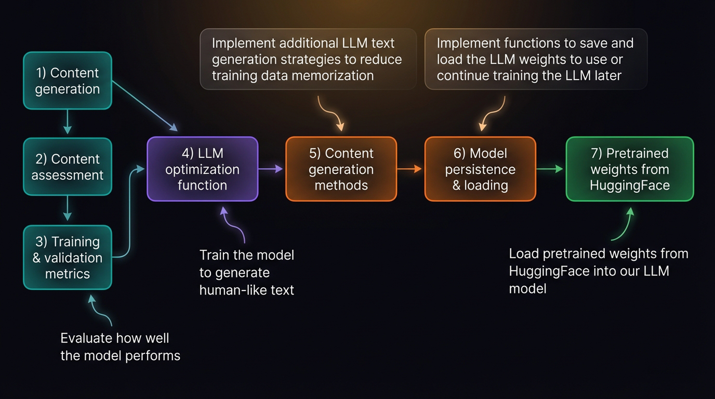
The seven steps: content generation → content assessment → training & validation metrics → LLM optimization function → content generation methods → model persistence & loading → pretrained weights from HuggingFace.
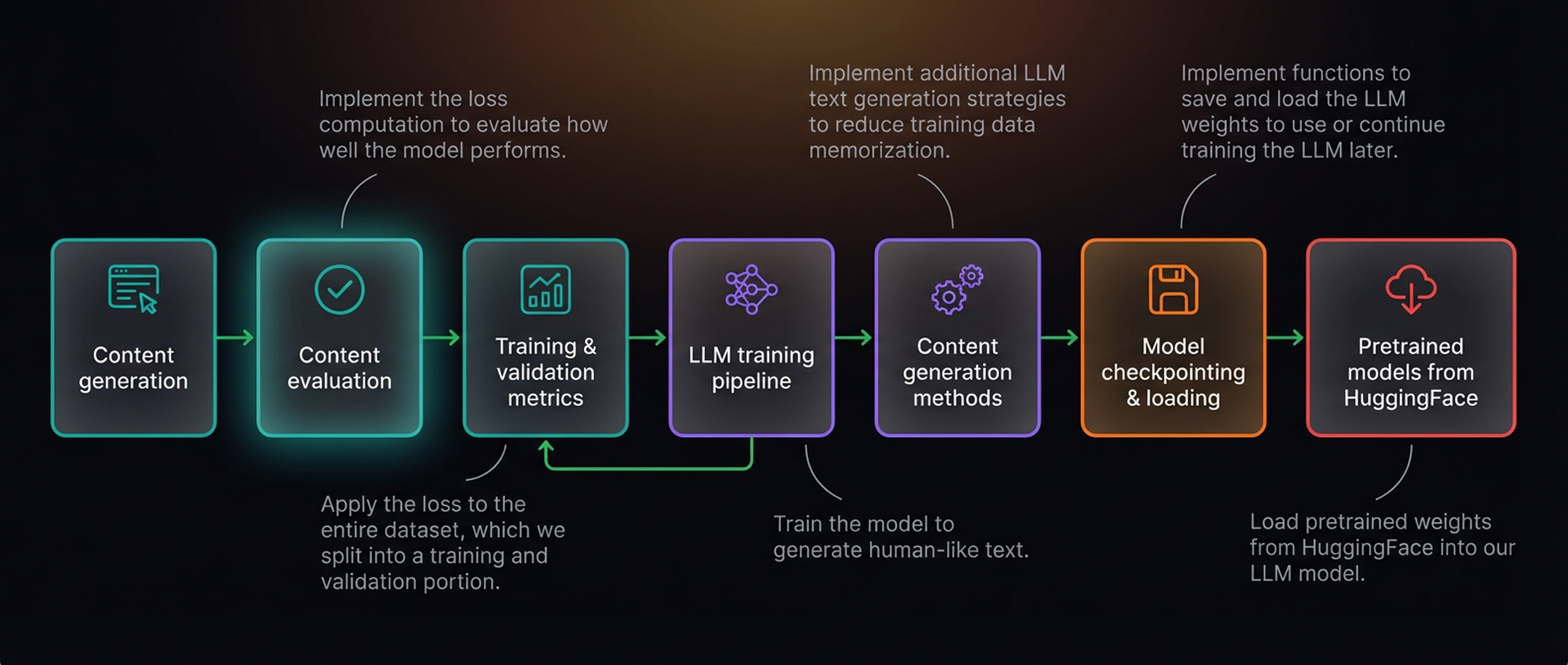
We also have a more detailed version with icons showing the same pipeline:
2. Generating Text with an Untrained Model
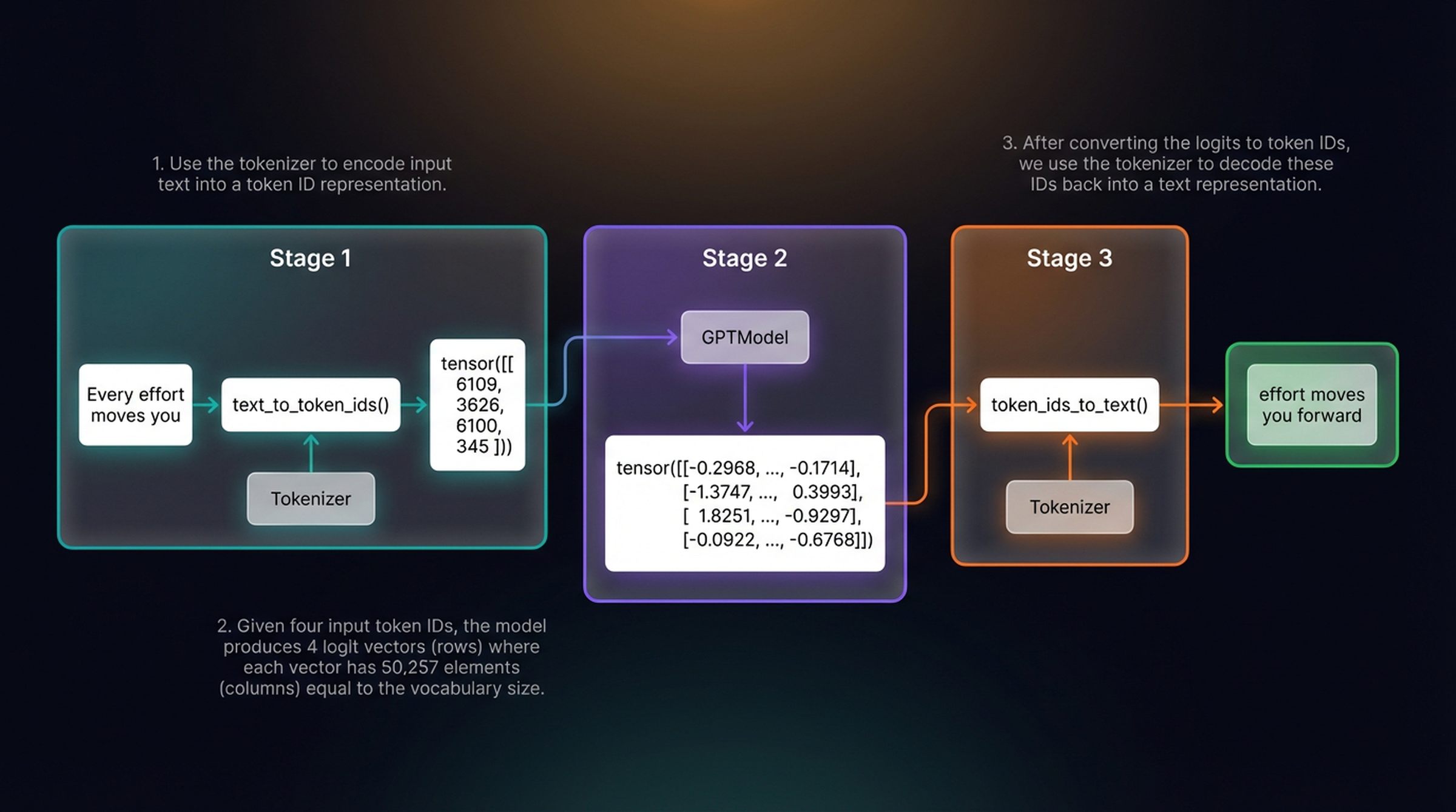
Before we can train anything, we need to understand what our untrained model produces. The text generation pipeline has three stages: encode text into token IDs, pass them through the GPT model to get logit vectors, then decode the output back into text.
The complete pipeline. Input text “Every effort moves you” is tokenized into IDs [6109, 3626, 6100, 345], processed by the GPTModel into logit vectors (4 rows × 50,257 columns), then decoded via token_ids_to_text() back into text.
Let’s set up our model and the essential conversion functions:
import torch
import tiktoken
from chapter04 import GPTModel

GPT_CONFIG_124M = {
    "vocab_size": 50257,
    "context_length": 256,    # Reduced from 1024 for training efficiency
    "emb_dim": 768,
    "n_heads": 12,
    "n_layers": 12,
    "drop_rate": 0.1,
    "qkv_bias": False
}

torch.manual_seed(123)
model = GPTModel(GPT_CONFIG_124M)
model.eval()

def text_to_token_ids(text, tokenizer):
    encoded = tokenizer.encode(text, allowed_special={'<|endoftext|>'})
    encoded_tensor = torch.tensor(encoded).unsqueeze(0)  # Add batch dim
    return encoded_tensor

def token_ids_to_text(token_ids, tokenizer):
    flat = token_ids.squeeze(0)  # Remove batch dim
    return tokenizer.decode(flat.tolist())
Let’s see what our randomly initialized model produces:
start_context = "Every effort moves you"
tokenizer = tiktoken.get_encoding("gpt2")

token_ids = generate_text_simple(
    model=model,
    idx=text_to_token_ids(start_context, tokenizer),
    max_new_tokens=10,
    context_size=GPT_CONFIG_124M["context_length"]
)

print("Output:", token_ids_to_text(token_ids, tokenizer))
# Output: Every effort moves you rentingetic wasn? refres RexMeCHicular stren
Complete nonsense — exactly what we expect from random weights. To fix this, we need a way to measure how bad the output is.
3. Measuring Quality: The Cross-Entropy Loss Pipeline
How do we quantify “nonsense” mathematically? For each input token, the model produces a probability distribution over the entire vocabulary. We want the probability assigned to the correct next token to be as high as possible.
Let’s first see this with a small toy vocabulary to build intuition. The figure below shows a 7-word vocabulary where input words “each”, “step”, “brings” are mapped to token IDs, processed through softmax to produce probability vectors, then argmax selects the highest-probability index:
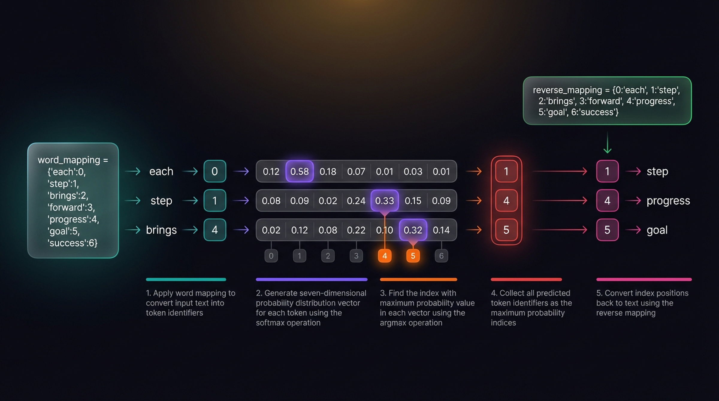
Text generation with a 7-word toy vocabulary: (1) map words to IDs, (2) generate probability vectors via softmax, (3) find the max probability index via argmax, (4) collect predicted token IDs, (5) convert back to text via reverse mapping. The model predicts “step → progress → goal”.
In practice, our GPT model uses a 50,257-token vocabulary. Let’s set up two training examples. The inputs and targets are shifted by one position — the model must predict each next token:
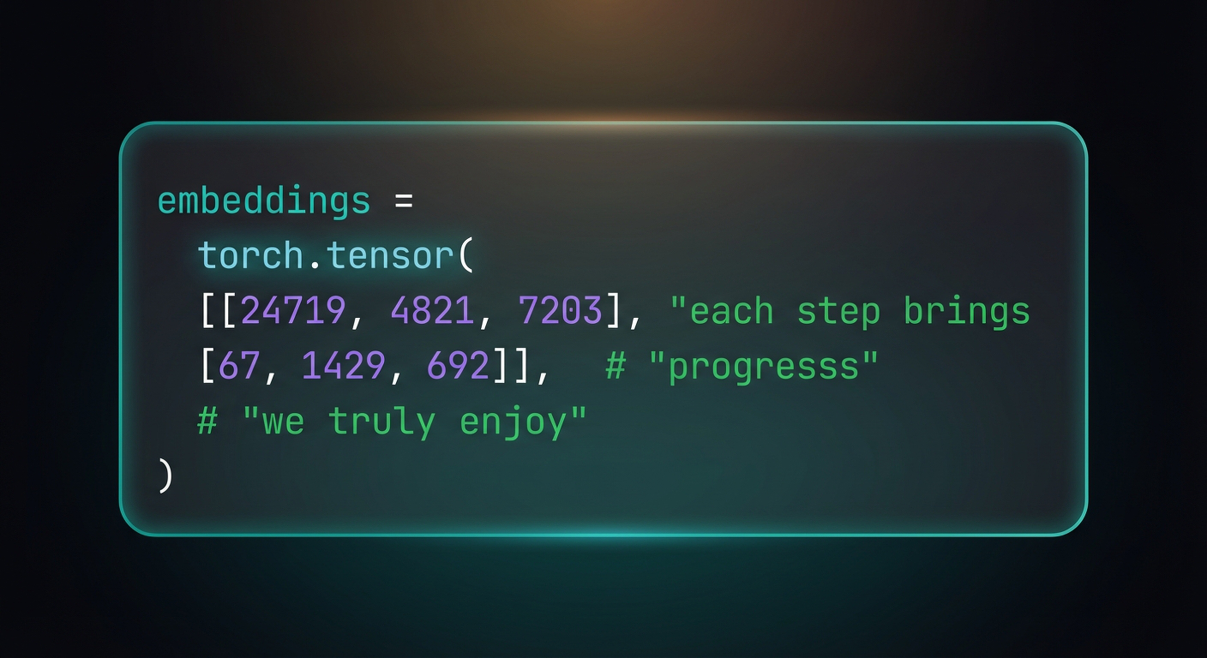
Our two training sequences as token ID tensors: [24719, 4821, 7203] for “each step brings” and [67, 1429, 692] for “we truly enjoy”.
# Two training sequences (matching the figure above)
sequences = torch.tensor([[24719, 4821, 7203],    # "each step brings"
                          [67,    1429, 692]])     # "we truly enjoy"

targets = torch.tensor([[4821, 7203, 16073],       # "step brings progress"
                        [1429, 692,  32945]])       # "truly enjoy learning"
We feed the sequences through the model and apply softmax to get probabilities. Notice how torch.no_grad() disables gradient tracking since we’re not training yet:
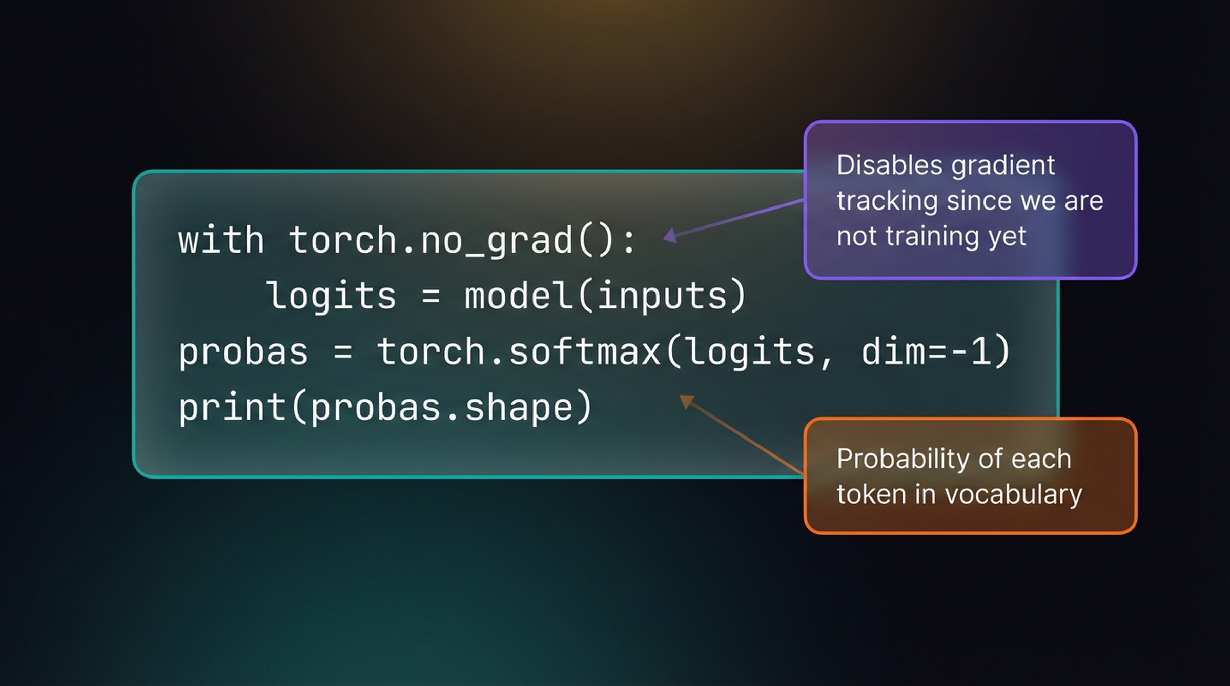
with torch.no_grad():
    logits = model(sequences)
probas = torch.softmax(logits, dim=-1)
print(probas.shape)  # torch.Size([2, 3, 50257])
From Probabilities to Loss
An untrained network produces roughly uniform random probability distributions. The training objective is to maximize the probabilities at the positions corresponding to the correct target tokens:
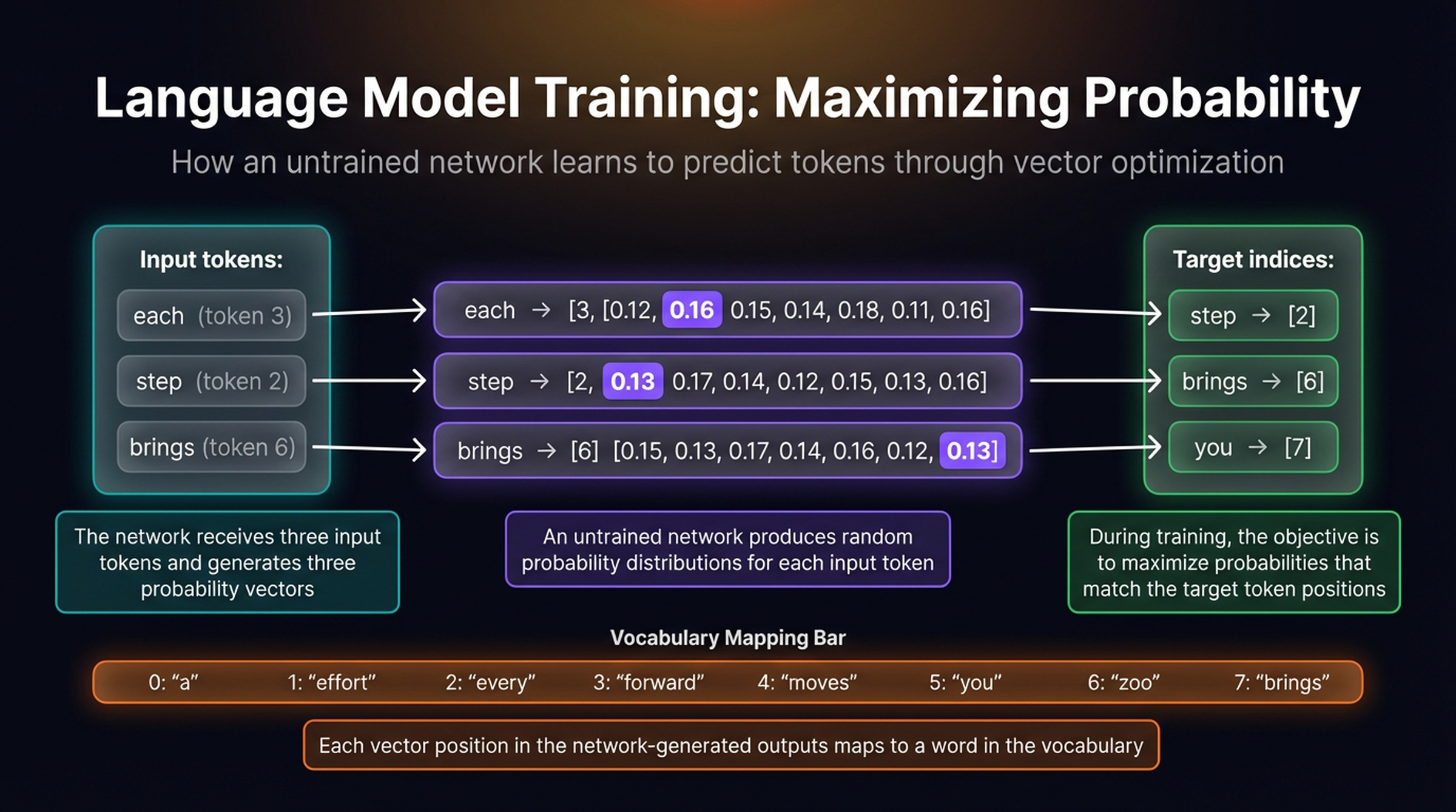
How training works: the network receives input tokens (“each”, “step”, “brings”) and produces random probability vectors. The goal is to maximize probabilities at the target positions (“step”, “brings”, “you”). Each position in the vector maps to a word in the vocabulary.
The loss computation follows six steps — from raw logits down to a single scalar we can optimize:
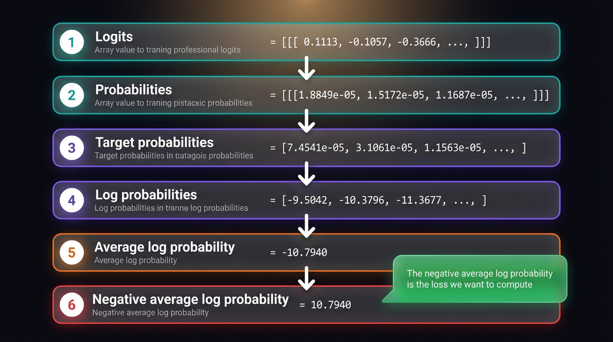
The complete loss pipeline: (1) raw logits, (2) softmax probabilities, (3) extract target probabilities, (4) take the logarithm, (5) compute the average, (6) negate it. The negative average log probability (10.7940) is our cross-entropy loss.
In practice, PyTorch’s cross_entropy handles all six steps:
# Manual approach (for understanding)
target_probas_1 = probas[0, [0, 1, 2], targets[0]]
target_probas_2 = probas[1, [0, 1, 2], targets[1]]
log_probas = torch.log(torch.cat((target_probas_1, target_probas_2)))
avg_log_probas = torch.mean(log_probas)
neg_avg_log_probas = avg_log_probas * -1
print(neg_avg_log_probas)  # tensor(10.7940)

# PyTorch shortcut (for production)
logits_flat = logits.flatten(0, 1)
targets_flat = targets.flatten()
loss = torch.nn.functional.cross_entropy(logits_flat, targets_flat)
print(loss)  # tensor(10.7940) — same result!
Perplexity: A related metric is perplexity = exp(loss). For our untrained model, that’s exp(10.794) ≈ 48,726 — meaning the model is equally uncertain among roughly 48,726 vocabulary tokens at each step.
4. Preparing Training Data
With evaluation in place, we can now prepare our training data. The roadmap shows where we are — steps 1-3 complete, moving into the training infrastructure:
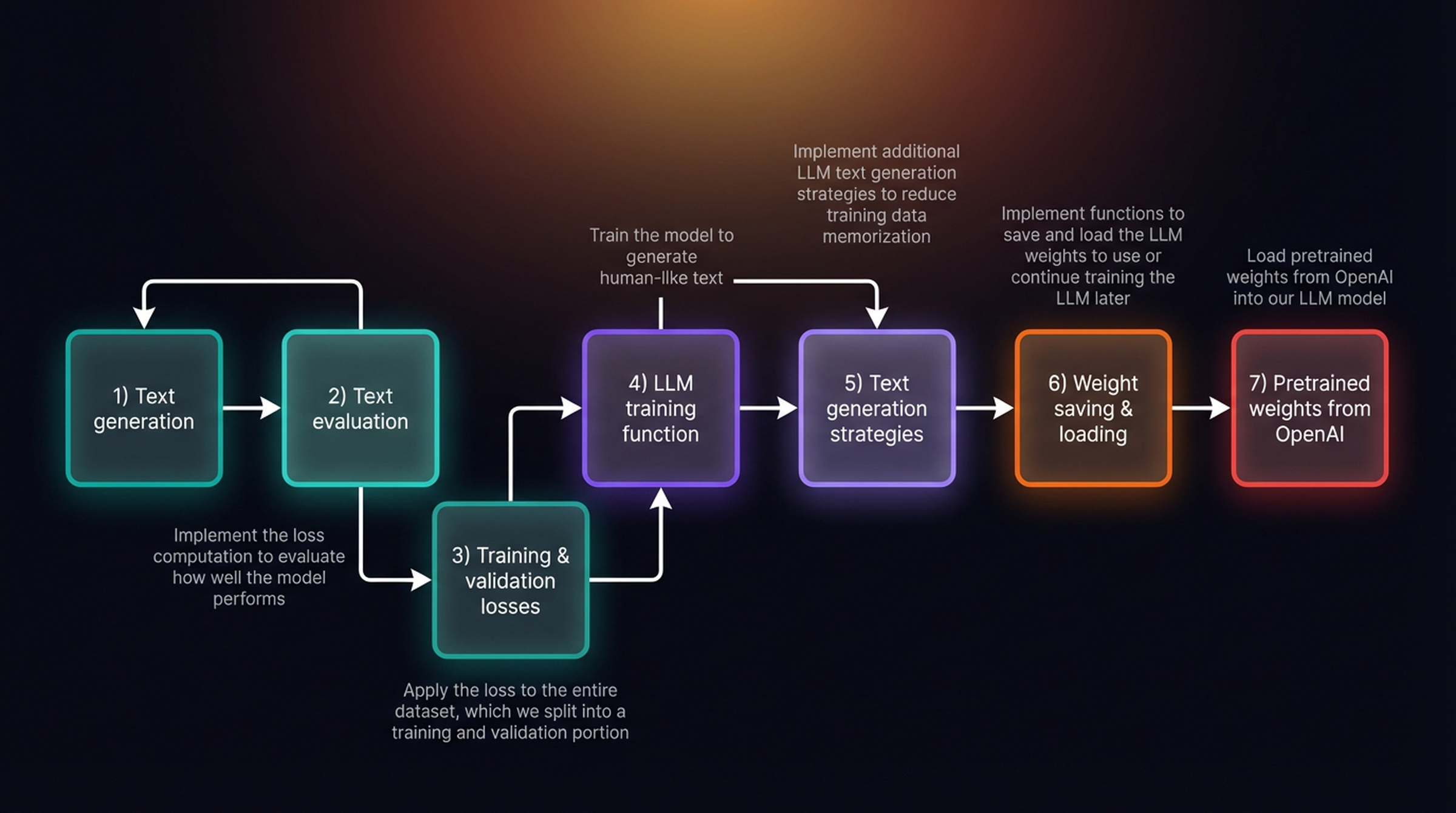
We’ll use “The Verdict” by Edith Wharton — a short public domain story with about 5,145 tokens. Tiny by LLM standards, but perfect for learning the mechanics on a laptop.
The data preparation pipeline tokenizes the raw text, chunks it into fixed-length sequences, and organizes those chunks into batches:
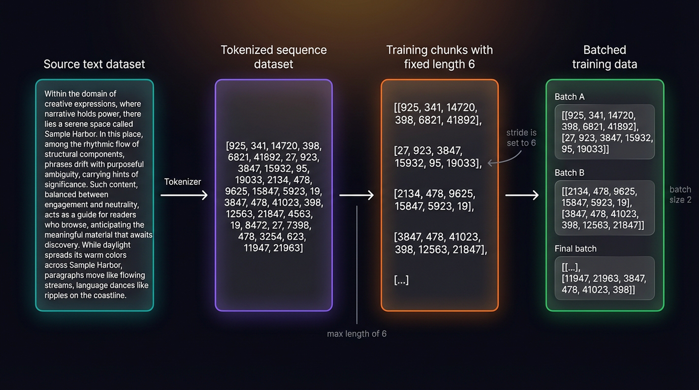
From raw text to batched training data. The tokenizer converts text into a long token ID sequence. We split this into fixed-length chunks (shown with length 6 for illustration; we use 256 in practice). Chunks are organized into batches of size 2 with shuffling enabled. Note the stride is set to 6 — matching the chunk length.
file_path = "the-verdict.txt"
with open(file_path, "r", encoding="utf-8") as file:
    text_data = file.read()

total_characters = len(text_data)
total_tokens = len(tokenizer.encode(text_data))
print("Characters:", total_characters)  # 20479
print("Tokens:", total_tokens)          # 5145

# 90/10 train/val split
train_ratio = 0.90
split_idx = int(train_ratio * len(text_data))
train_data = text_data[:split_idx]
val_data = text_data[split_idx:]

from chapter02 import create_dataloader_v1

torch.manual_seed(123)
train_loader = create_dataloader_v1(
    train_data, batch_size=2,
    max_length=GPT_CONFIG_124M["context_length"],
    stride=GPT_CONFIG_124M["context_length"],
    drop_last=True, shuffle=True, num_workers=0
)

val_loader = create_dataloader_v1(
    val_data, batch_size=2,
    max_length=GPT_CONFIG_124M["context_length"],
    stride=GPT_CONFIG_124M["context_length"],
    drop_last=False, shuffle=False, num_workers=0
)
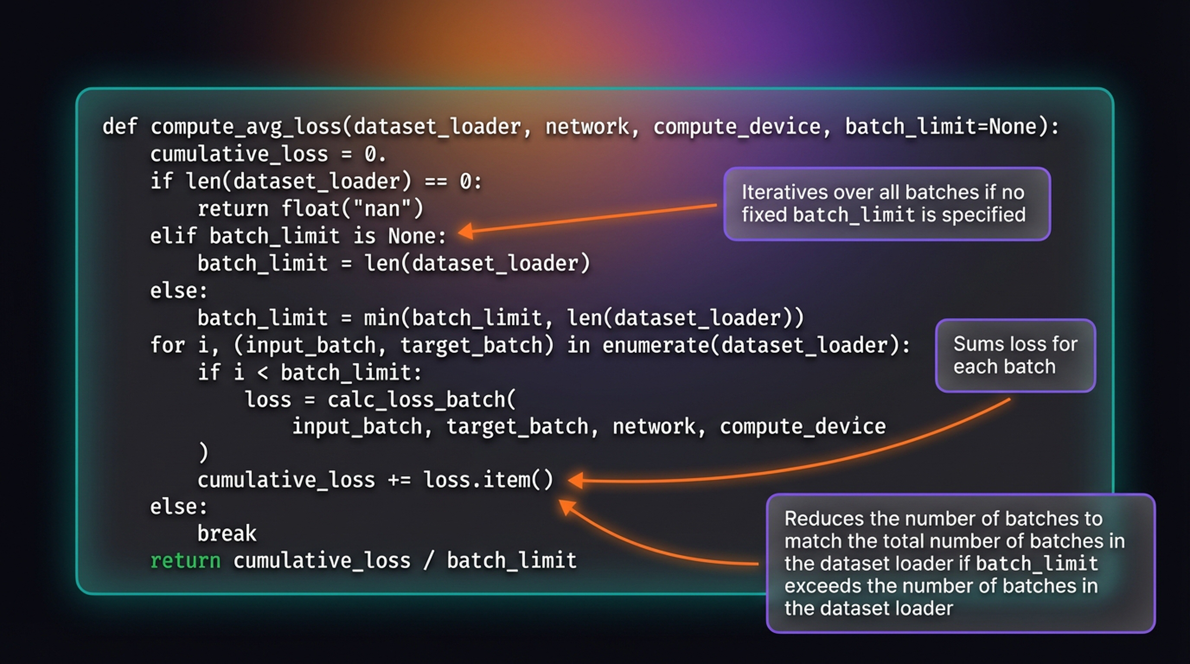
Now we need utility functions to compute the average loss across all batches in a data loader. The figure below shows the annotated function — notice how it handles edge cases and supports a batch_limit parameter for faster evaluation:
def calc_loss_batch(input_batch, target_batch, model, device):
    input_batch = input_batch.to(device)
    target_batch = target_batch.to(device)
    logits = model(input_batch)
    loss = torch.nn.functional.cross_entropy(
        logits.flatten(0, 1), target_batch.flatten()
    )
    return loss

def calc_loss_loader(data_loader, model, device, num_batches=None):
    total_loss = 0.
    if len(data_loader) == 0:
        return float("nan")
    elif num_batches is None:
        num_batches = len(data_loader)
    else:
        num_batches = min(num_batches, len(data_loader))
    for i, (input_batch, target_batch) in enumerate(data_loader):
        if i < num_batches:
            loss = calc_loss_batch(input_batch, target_batch, model, device)
            total_loss += loss.item()
        else:
            break
    return total_loss / num_batches
Here’s the roadmap showing our progress — the first three steps checked off:
Let’s compute the initial losses before any training. The figure shows the annotated code with automatic GPU detection:
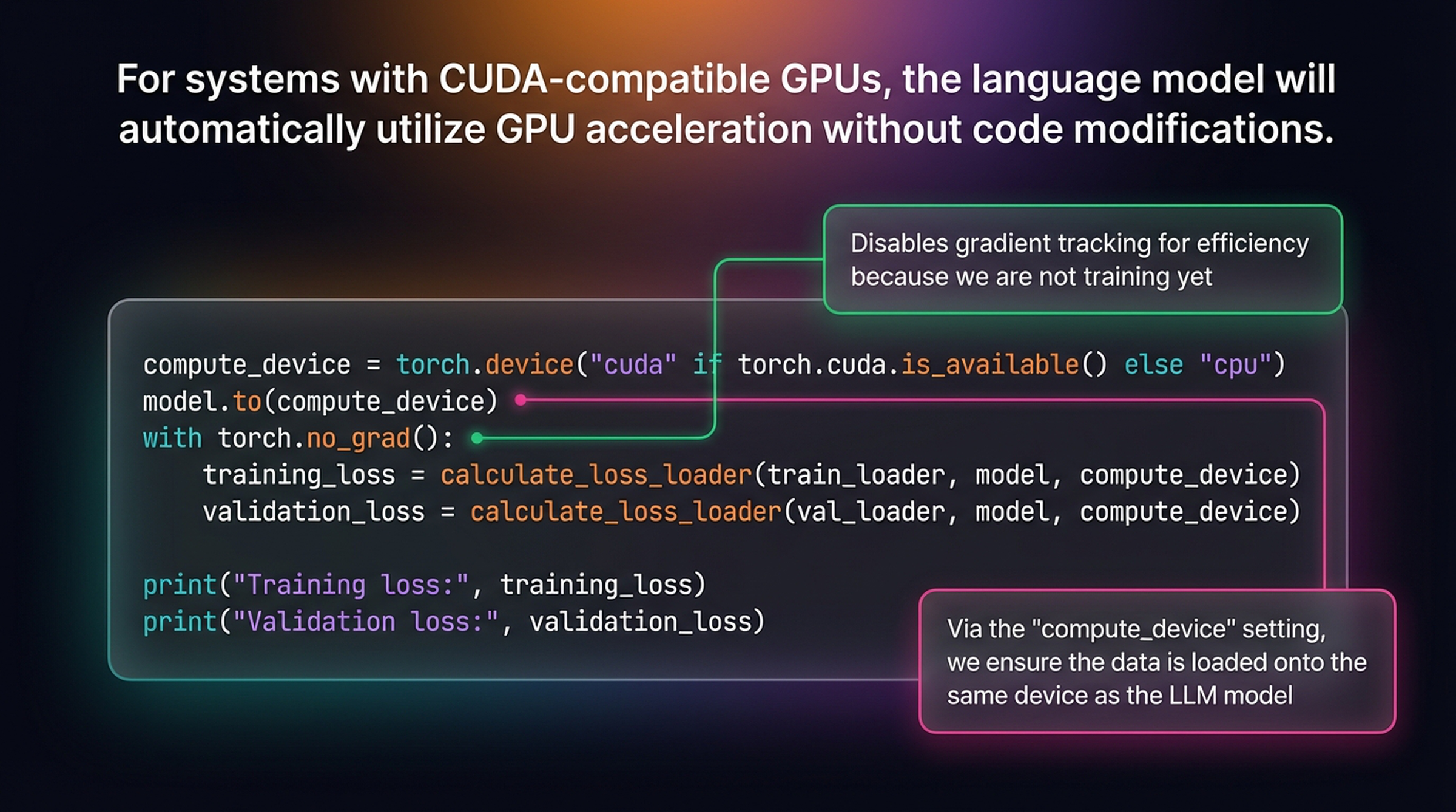
device = torch.device("cuda" if torch.cuda.is_available() else "cpu")
model.to(device)

with torch.no_grad():
    train_loss = calc_loss_loader(train_loader, model, device)
    val_loss = calc_loss_loader(val_loader, model, device)

print("Training loss:", train_loss)    # ~10.99
print("Validation loss:", val_loss)    # ~10.98
Both losses hover around 10.98 — very high. For reference, a loss near 0 means the model perfectly predicts every next token. Time to train.
5. The Training Loop
The training loop follows the standard PyTorch deep learning recipe. Here’s the high-level flow as a flowchart — eight steps from iterating over epochs to generating sample text:
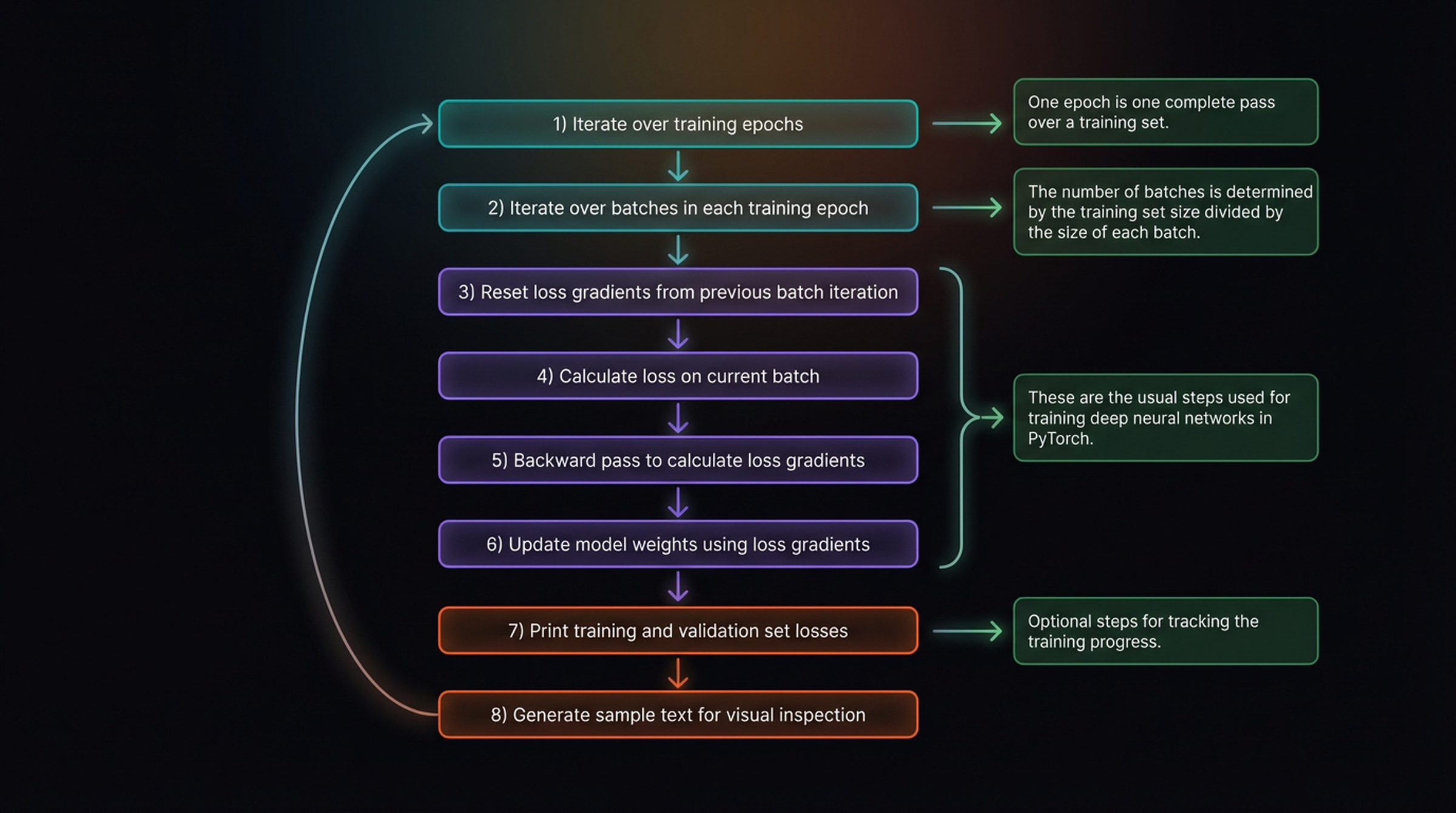
The standard training loop. Steps 1–6 (teal/purple) are the core optimization cycle used for any PyTorch neural network. Steps 7–8 (orange) are optional monitoring steps for tracking progress.
Now the full annotated implementation. Compare the code in the figure with what follows — the logic is the same:
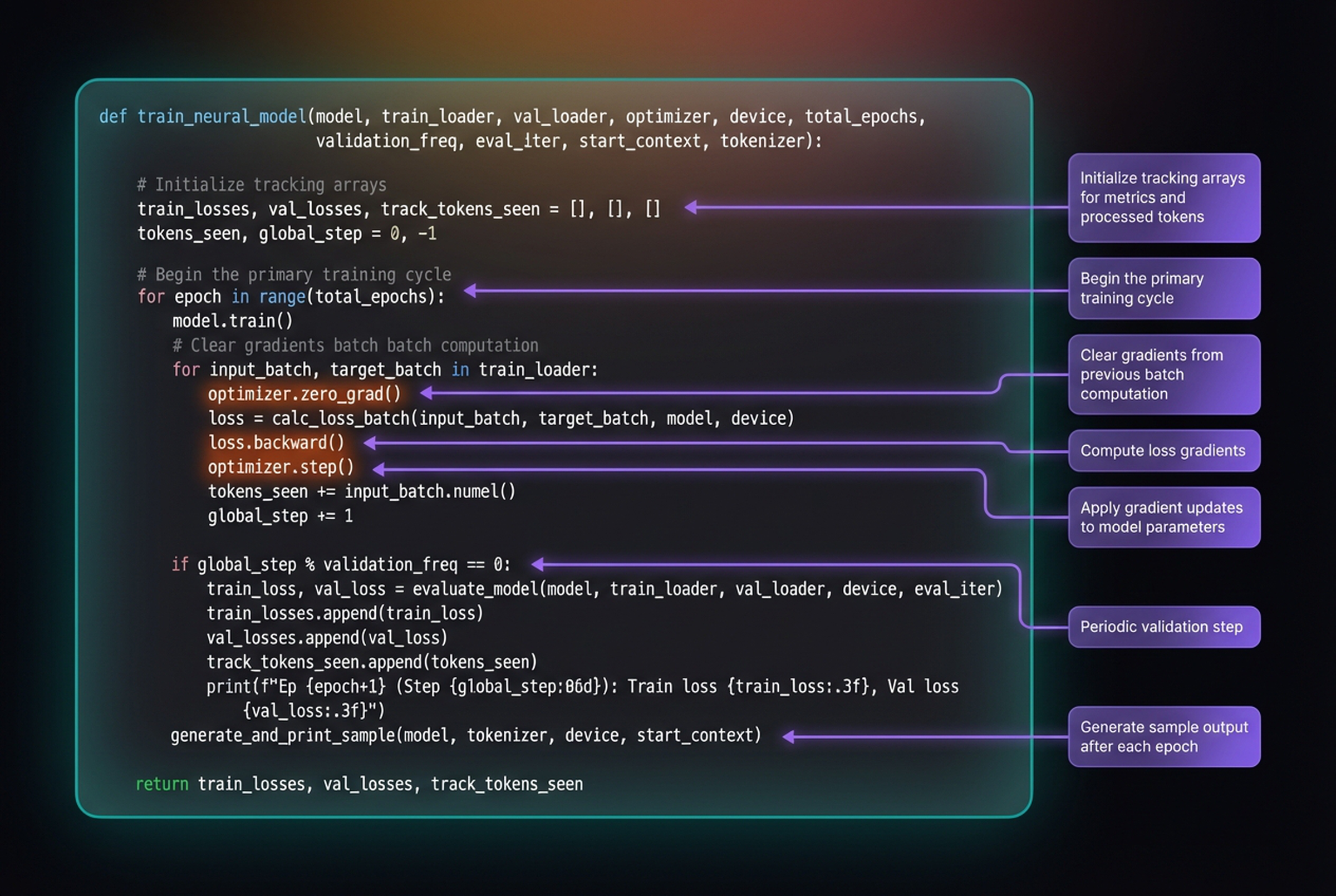
The complete training function: initialize tracking arrays, begin the epoch loop, clear gradients, compute loss, backpropagate, update weights, periodically evaluate, and generate sample text after each epoch.
def train_model_simple(model, train_loader, val_loader,
                       optimizer, device, num_epochs,
                       eval_freq, eval_iter, start_context, tokenizer):
    train_losses, val_losses, track_tokens_seen = [], [], []
    tokens_seen, global_step = 0, -1

    for epoch in range(num_epochs):
        model.train()
        for input_batch, target_batch in train_loader:
            optimizer.zero_grad()
            loss = calc_loss_batch(input_batch, target_batch, model, device)
            loss.backward()
            optimizer.step()
            tokens_seen += input_batch.numel()
            global_step += 1

            if global_step % eval_freq == 0:
                train_loss, val_loss = evaluate_model(
                    model, train_loader, val_loader, device, eval_iter)
                train_losses.append(train_loss)
                val_losses.append(val_loss)
                track_tokens_seen.append(tokens_seen)
                print(f"Ep {epoch+1} (Step {global_step:06d}): "
                      f"Train loss {train_loss:.3f}, Val loss {val_loss:.3f}")

        generate_and_print_sample(model, tokenizer, device, start_context)

    return train_losses, val_losses, track_tokens_seen

def evaluate_model(model, train_loader, val_loader, device, eval_iter):
    model.eval()
    with torch.no_grad():
        train_loss = calc_loss_loader(
            train_loader, model, device, num_batches=eval_iter)
        val_loss = calc_loss_loader(
            val_loader, model, device, num_batches=eval_iter)
    model.train()
    return train_loss, val_loss

def generate_and_print_sample(model, tokenizer, device, start_context):
    model.eval()
    context_size = model.pos_emb.weight.shape[0]
    encoded = text_to_token_ids(start_context, tokenizer).to(device)
    with torch.no_grad():
        token_ids = generate_text_simple(
            model=model, idx=encoded,
            max_new_tokens=50, context_size=context_size)
    decoded_text = token_ids_to_text(token_ids, tokenizer)
    print(decoded_text.replace("\n", " "))
    model.train()
Let’s launch the training:
torch.manual_seed(123)
model = GPTModel(GPT_CONFIG_124M)
model.to(device)

optimizer = torch.optim.AdamW(
    model.parameters(), lr=0.0004, weight_decay=0.1
)

num_epochs = 10
train_losses, val_losses, tokens_seen = train_model_simple(
    model, train_loader, val_loader, optimizer, device,
    num_epochs=num_epochs, eval_freq=5, eval_iter=5,
    start_context="Every effort moves you", tokenizer=tokenizer
)
Watch the transformation unfold:
# Epoch 1:  "Every effort moves you,,,,,,,,,,,,,."
# Epoch 2:  "Every effort moves you, and, and, and, and, and..."
# ...
# Epoch 9:  'Every effort moves you?" "Yes--quite insensible to the irony...'
# Epoch 10: 'Every effort moves you know," was one of the axioms he laid
#            down across the Sevres and silver of an exquisitely appointed...'
The training and validation loss curves tell the full story:
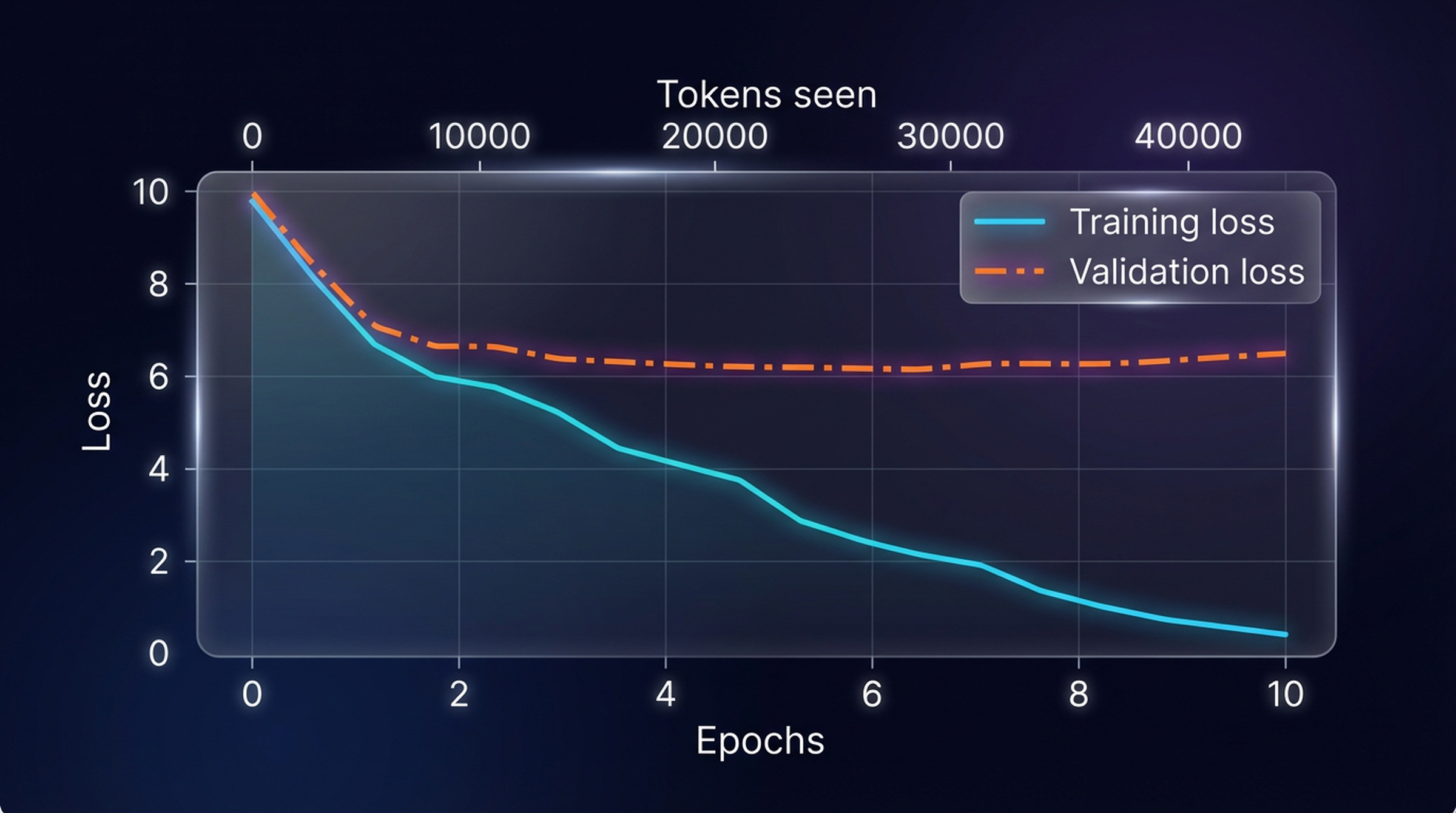
Training loss drops steadily from ~10 to near 0, while validation loss plateaus around 6.3 after epoch 2. The divergence signals overfitting — the model memorizes the tiny training set. This is expected with only 5,145 tokens.
Here’s where we stand after completing the training loop — steps 1-4 done, with the model generating coherent (but memorized) text:
6. Beyond Greedy Decoding: Temperature and Top-k
Our trained model always produces the same output for a given prompt — it greedily selects the highest-probability token at each step. This leads to repetitive, memorized text. Two techniques help: temperature scaling and top-k sampling.
Temperature Scaling
Temperature is simple: divide the logits by a scalar before applying softmax. Lower temperatures sharpen the distribution (more deterministic), higher temperatures flatten it (more diverse).
def softmax_with_temperature(logits, temperature):
    scaled_logits = logits / temperature
    return torch.softmax(scaled_logits, dim=0)

# Example logits for next token
next_token_logits = torch.tensor(
    [4.51, 0.89, -1.90, 6.75, 1.63, -1.62, -1.89, 6.28, 1.79]
)

temperatures = [1, 0.1, 5]
for T in temperatures:
    probs = softmax_with_temperature(next_token_logits, T)
    print(f"T={T}: max prob = {probs.max():.3f}")
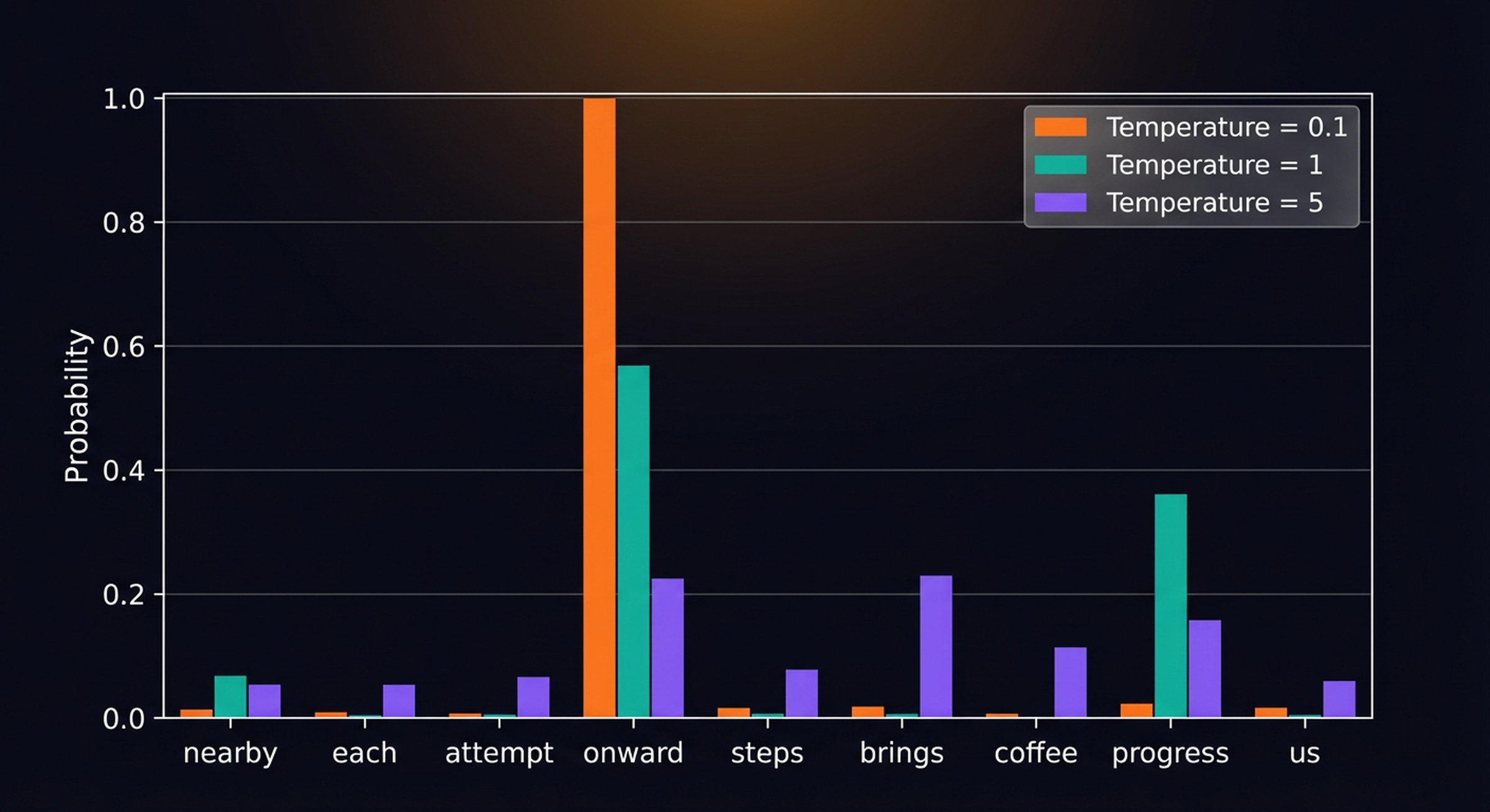
Temperature scaling in action. At T=0.1, the top token gets nearly 100% probability (almost deterministic). At T=1.0, the original distribution is preserved. At T=5.0, the distribution flattens — less likely tokens get meaningful probability mass.
Top-k Sampling
Temperature alone can produce nonsensical outputs. Top-k sampling restricts candidate tokens to only the k most likely ones, masking everything else with negative infinity before applying softmax:
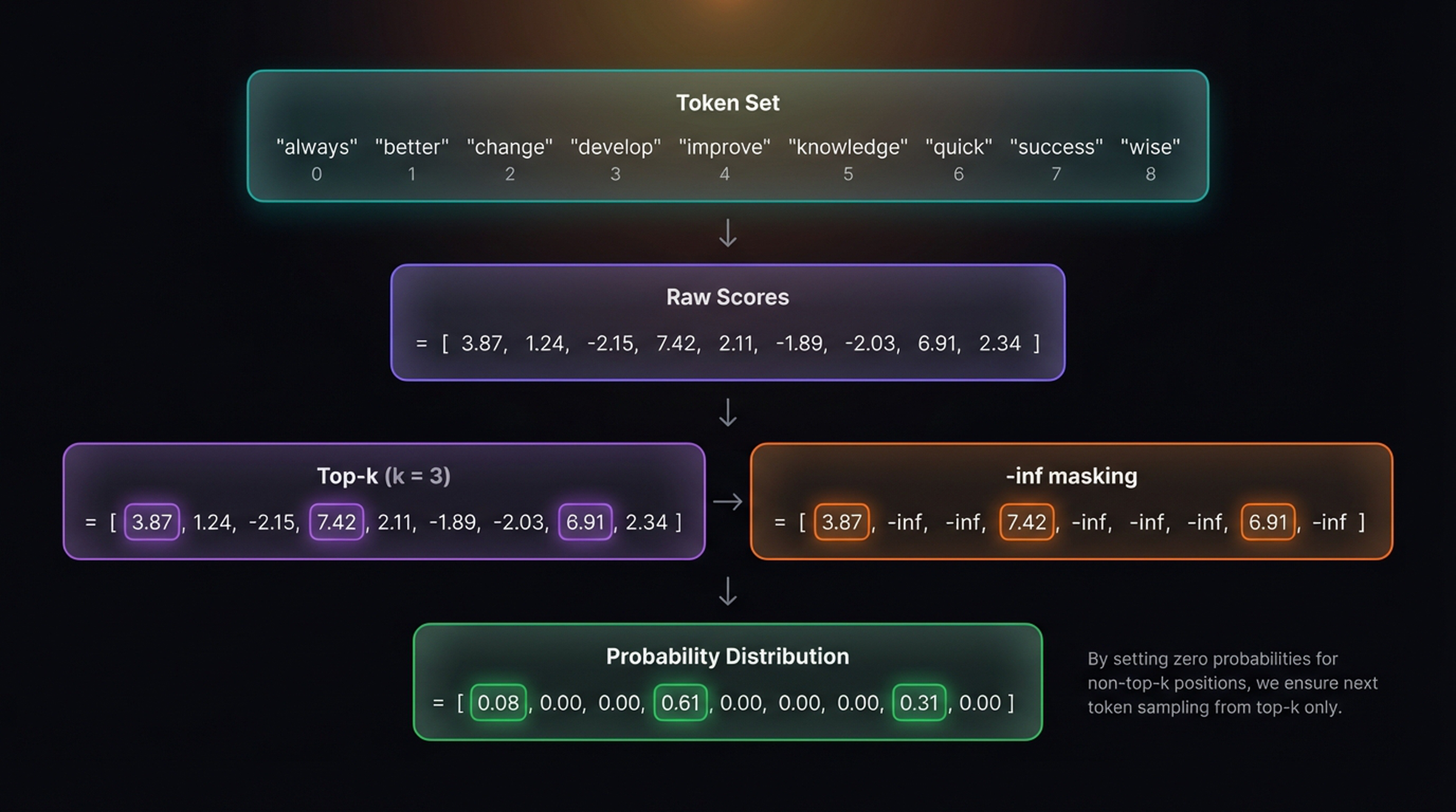
Top-k sampling with k=3. From the raw logits, we identify the three highest values, mask all others with -inf, and apply softmax. Only three tokens retain non-zero probability.
The actual tensor after top-k masking: only three positions retain their original logit values, all others are -inf.
Here’s the combined generation function with both techniques:
def generate(model, idx, max_new_tokens, context_size,
             temperature=0.0, top_k=None, eos_id=None):
    for _ in range(max_new_tokens):
        idx_cond = idx[:, -context_size:]
        with torch.no_grad():
            logits = model(idx_cond)
        logits = logits[:, -1, :]

        # Top-k filtering
        if top_k is not None:
            top_logits, _ = torch.topk(logits, top_k)
            min_val = top_logits[:, -1]
            logits = torch.where(
                logits < min_val,
                torch.tensor(float('-inf')).to(logits.device),
                logits
            )

        # Temperature scaling + multinomial sampling
        if temperature > 0.0:
            logits = logits / temperature
            probs = torch.softmax(logits, dim=-1)
            idx_next = torch.multinomial(probs, num_samples=1)
        else:
            idx_next = torch.argmax(logits, dim=-1, keepdim=True)

        if idx_next == eos_id:
            break
        idx = torch.cat((idx, idx_next), dim=1)
    return idx
torch.manual_seed(123)
token_ids = generate(
    model=model,
    idx=text_to_token_ids("Every effort moves you", tokenizer),
    max_new_tokens=15,
    context_size=GPT_CONFIG_124M["context_length"],
    top_k=25,
    temperature=1.4
)
print(token_ids_to_text(token_ids, tokenizer))
# "Every effort moves you stand to work on surprise, a one of us had gone with random-"
Much more diverse than the memorized output from greedy decoding.
7. Saving, Loading, and Professional Weights
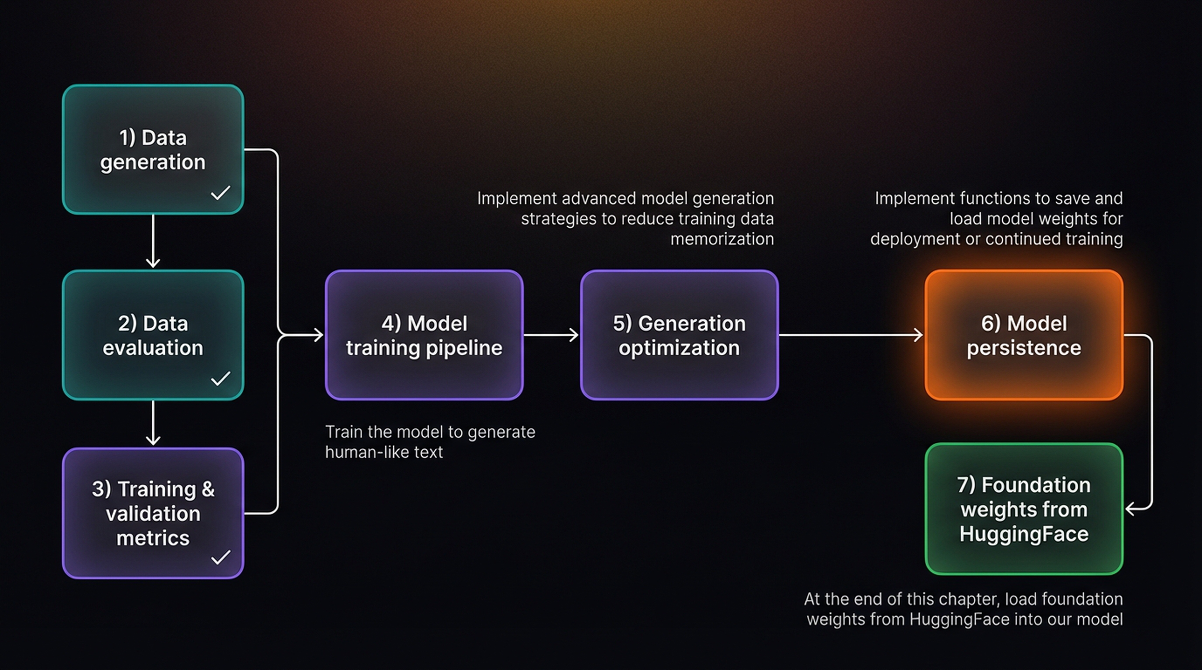
We’re now in the final stretch of our roadmap:
Model Checkpointing
Training is expensive — always save your work:
# Save model weights only
torch.save(model.state_dict(), "model.pth")

# Save everything for resuming training later
torch.save({
    "model_state_dict": model.state_dict(),
    "optimizer_state_dict": optimizer.state_dict(),
}, "model_and_optimizer.pth")

# Restore a saved model
model = GPTModel(GPT_CONFIG_124M)
model.load_state_dict(torch.load("model.pth", map_location=device))
model.eval()
Loading Pretrained GPT-2 Weights
The real power comes from loading professionally pretrained weights into our architecture. First, download the weights:
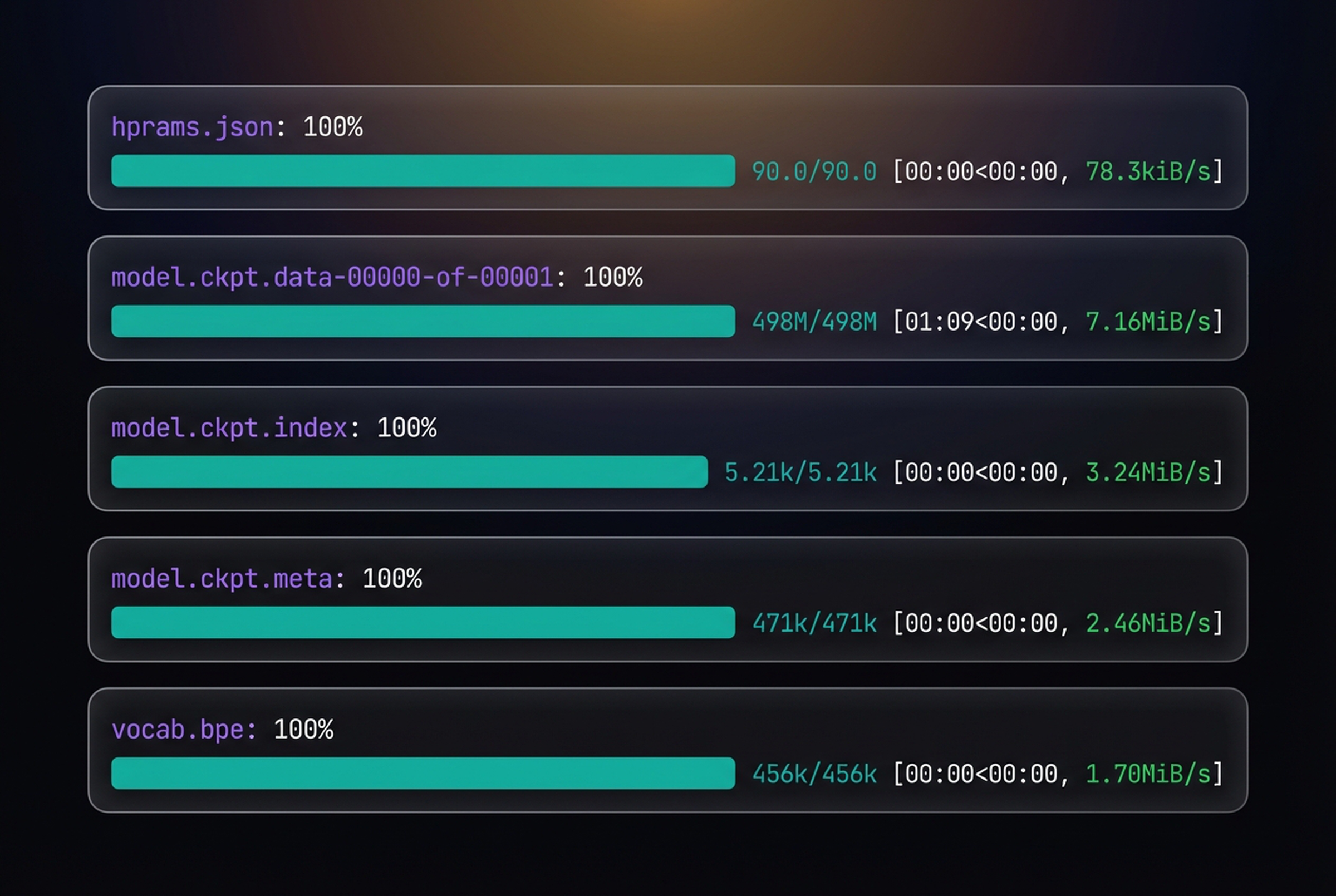
from gpt_download import download_and_load_gpt2

settings, params = download_and_load_gpt2(
    model_size="124M", models_dir="gpt2"
)

print("Settings:", settings)
print("Parameter keys:", params.keys())
OpenAI released weights for four GPT-2 model sizes. They all share the same core architecture — the differences are in embedding dimensions, number of transformer blocks, and attention heads:
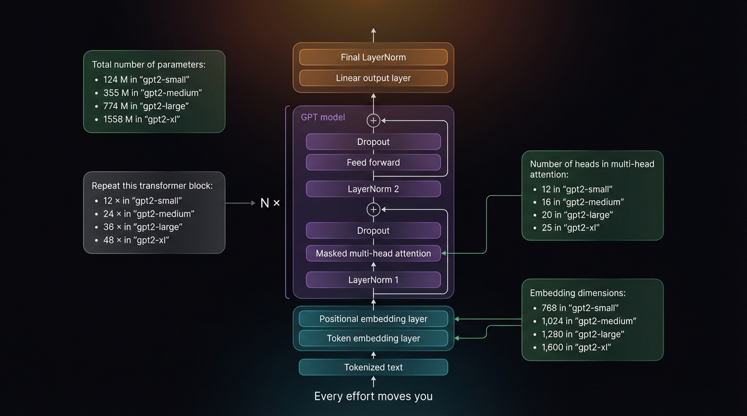
The GPT-2 model family. All four sizes share the same architecture: token + positional embeddings → N transformer blocks (each with masked multi-head attention + feedforward) → final LayerNorm → linear output. The differences: 768→1600 embedding dims, 12→48 blocks, 12→25 attention heads, 124M→1558M total parameters.
The weight loading function maps OpenAI’s naming convention to our GPTModel. The key insight: OpenAI stores Q, K, V attention weights as a single concatenated matrix that we split into three parts using np.split:
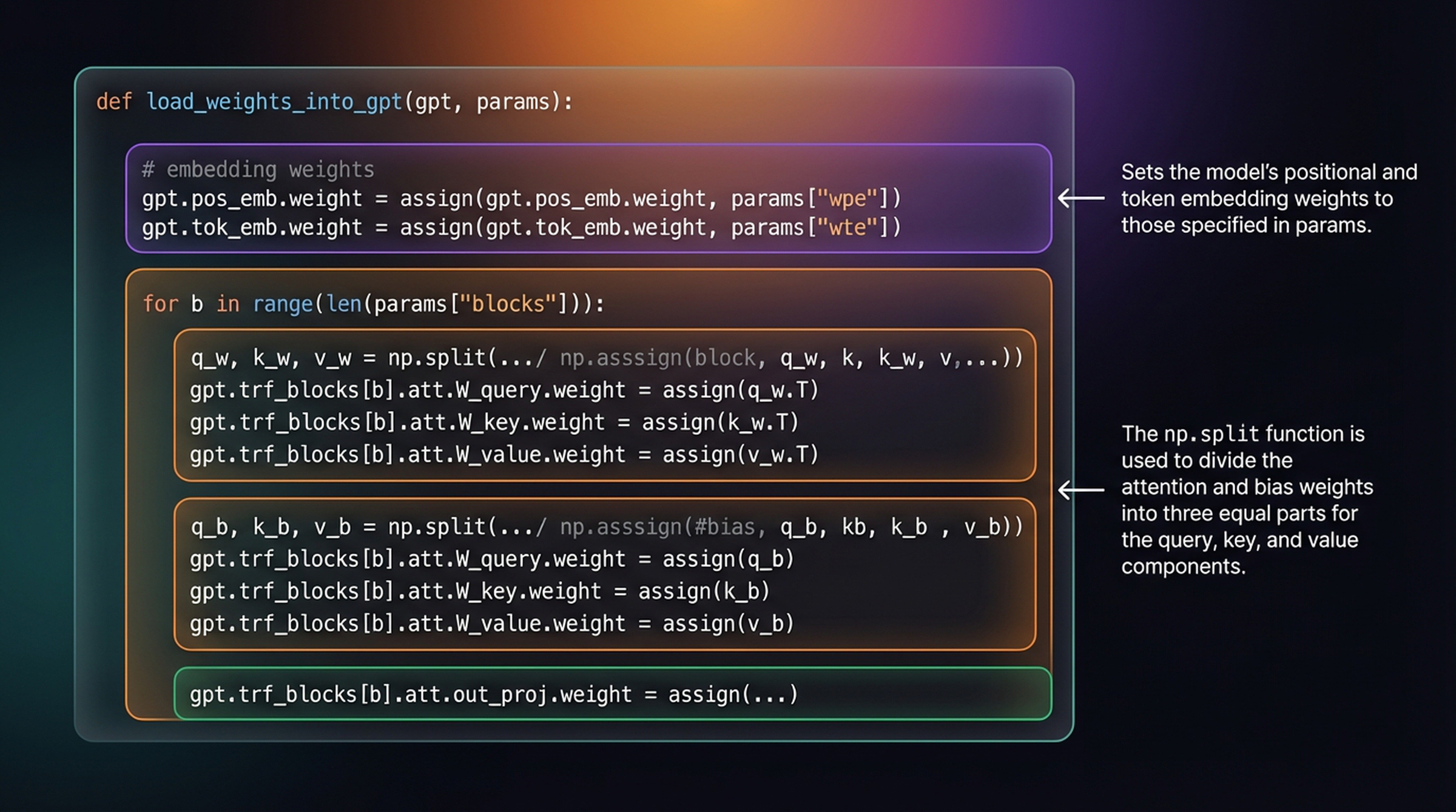
The weight loading function: assign positional and token embedding weights, then iterate through each transformer block splitting the combined attention weights into separate query, key, and value components.
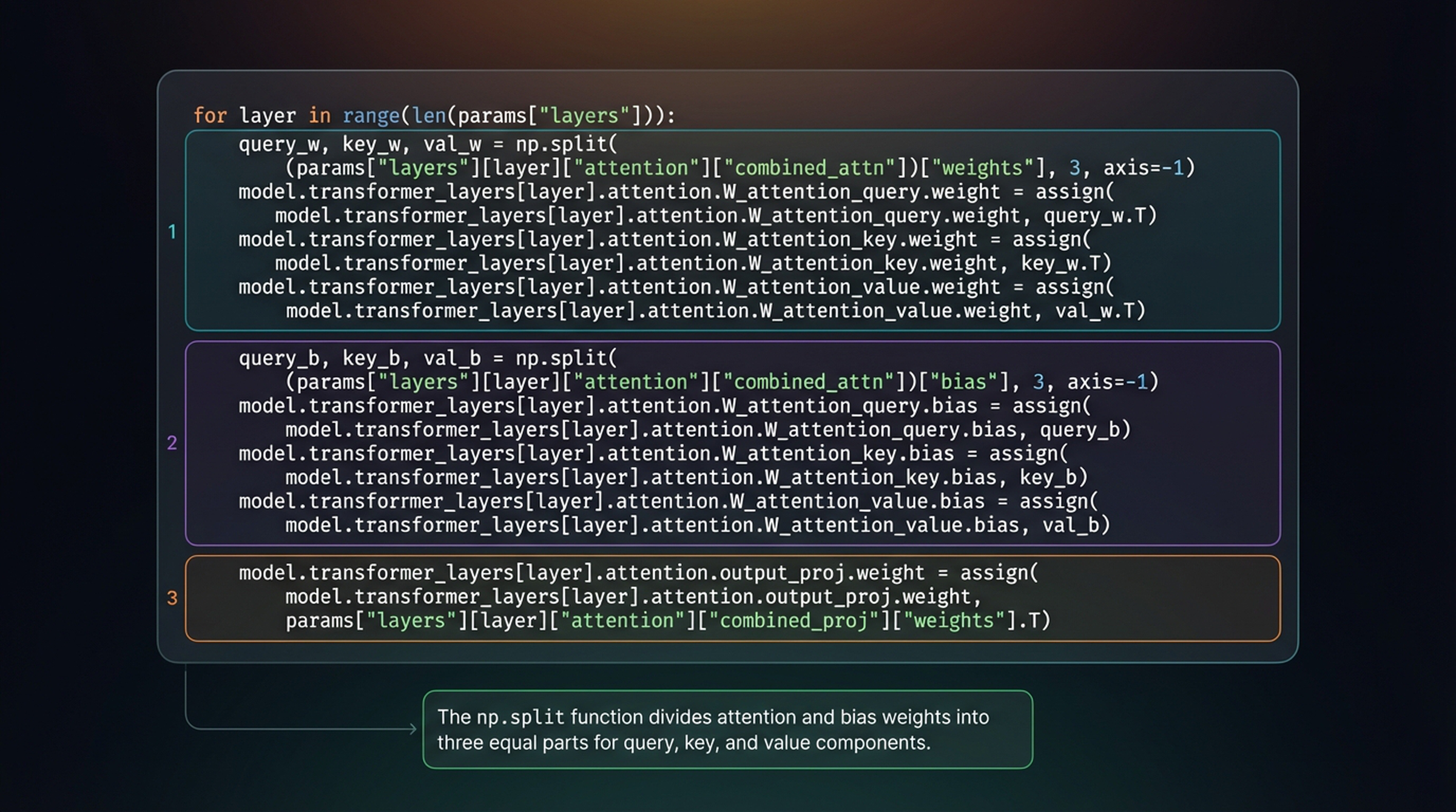
The full attention weight loading: for each transformer layer, (1) split combined attention weights into Q, K, V and assign transposed, (2) split combined biases, (3) assign output projection, feedforward, and layer normalization weights.
# Update config for pretrained model
NEW_CONFIG = GPT_CONFIG_124M.copy()
NEW_CONFIG.update({
    "context_length": 1024,   # Full GPT-2 context
    "qkv_bias": True,         # OpenAI models use bias
})

gpt = GPTModel(NEW_CONFIG)
load_weights_into_gpt(gpt, params)
gpt.to(device)
gpt.eval()

# Generate with professional weights
torch.manual_seed(123)
token_ids = generate(
    model=gpt,
    idx=text_to_token_ids("Every effort moves you", tokenizer).to(device),
    max_new_tokens=25,
    context_size=NEW_CONFIG["context_length"],
    top_k=50,
    temperature=1.5
)

print(token_ids_to_text(token_ids, tokenizer))
# "Every effort moves you toward finding an ideal new way to practice something!
#  What makes us want to be on top of that?"
The difference is stark. Our tiny model trained on 5,145 tokens produces grammatically correct but clearly memorized text from the training story. The professional GPT-2 model, trained on billions of tokens, generates genuinely novel, contextually rich language.
What You’ve Accomplished
You’ve implemented a complete LLM pretraining pipeline from scratch. Starting from an architecture that produced “rentingetic wasn? refres RexMeCHicular stren”, you built the machinery to transform random weights into a system that generates coherent text — and then went further by loading professional-grade weights.
Key takeaways: the training loop is standard PyTorch (zero grad → forward → loss → backward → step), but the loss function is cross-entropy over next-token predictions. Temperature and top-k sampling are essential for generating diverse outputs rather than memorized text. And model checkpointing is critical because training is expensive.