LLMs from Scratch #005: Mastering GPU Performance: From CUDA Fundamentals to Flash Attention
🎯 What You’ll Learn
In this comprehensive guide, we’ll demystify GPU hardware optimization for machine learning workloads. You’ll discover why GPUs exhibit mysterious performance patterns, understand the fundamental architectural differences between CPUs and GPUs, master six critical optimization techniques including low precision computation and operator fusion, and learn how Flash Attention cleverly combines tiling and recomputation to enable longer context windows in transformers. By the end, you’ll have the knowledge to write efficient CUDA kernels and optimize your deep learning models for maximum hardware utilization.
Tutorial Overview
- Course Introduction and Overview – Understanding GPU mysteries, course structure, and compute scaling fundamentals
- Historical Context of Parallel Computing – Evolution from Dennard scaling to GPU scaling
- GPU vs CPU Architecture Comparison – Architectural differences, execution units, and memory hierarchy
- GPU Execution and Memory Models – Blocks, warps, threads, and logical memory organization
- Performance Optimization Foundations – Roofline model and optimization strategy overview
- Low Precision Computation – Benefits of FP16/BF16 and arithmetic intensity improvements
- Operator Fusion Techniques – Memory access optimization through kernel fusion
- Memory Management Strategies – Recomputation and activation management
- Memory Access Pattern Optimization – Coalescing fundamentals and matrix multiplication
- Flash Attention Implementation – Tiling strategies, incremental softmax, and complete implementation
1. Course Introduction and Overview
Course Goals and Structure
Welcome to our deep dive into the world of GPUs – the powerhouse hardware that makes our language models possible. You may also check our previous posts [1], [2], [3] and [4]. If you haven’t really studied the hardware that makes your models run, GPUs can seem pretty mysterious and magical. You’ll get to implement Flash attention two or parts of Flash attention two, which I think will be nice, but first we need to understand what’s happening under the hood. My goal today is to make CUDA and GPUs less magic by helping you understand why GPUs get slow in very mysterious ways.
💡 The Performance Mystery
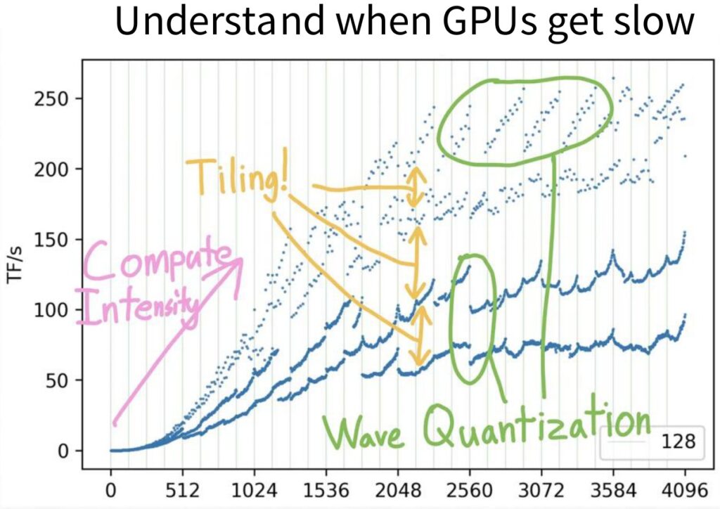
As you increase the size of your matrix multiplies, you might expect performance to scale predictably – either getting slower or faster in some consistent way. Instead, you get these very unpredictable looking wave-like patterns that leave you wondering why your GPU is fast at certain multiples of certain numbers and slow at others. Understanding these performance characteristics is crucial for developing efficient algorithms.
Understanding Flash Attention
The second major goal is understanding how to make fast algorithms like Flash attention, which makes much longer context possible by very cleverly computing the attention operation inside a transformer. Maybe you’d like to come up with new algorithms or new implementations like Flash attention – so what primitives and components do we need to understand to be able to do that?
There are great resources out there, including blogs with fun GPU facts that explain why matrix multiplies filled with zeros are faster than ones that aren’t, plus resources from the CUDA mode group and Google’s TPU book.
By the end of this lecture, you should feel comfortable with GPUs and understand how they work at a fundamental level. More importantly, you should feel confident about accelerating certain parts of your algorithms – when you create a new architecture, you should hopefully feel like you can try to accelerate that with CUDA. This foundation will be essential as we explore the specific performance characteristics and scaling behaviors that drive modern deep learning.
Performance Context and Compute Scaling
Building on our course goals, let’s now examine the structured approach we’ll take to understand GPU performance. Our exploration will be organized in three main parts: first, we’ll study GPUs in depth, examining how they work and their important components. I’ll also touch briefly on TPUs since they share many conceptual similarities with GPUs. Second, once we grasp the hardware and execution model of GPUs, we’ll analyze what makes them fast on certain workloads and what causes them to slow down, giving us a comprehensive understanding of GPU performance characteristics.
The third part will be our hands-on piece where we’ll put it all together by unpacking FlashAttention. I’ll walk you through this important algorithm, showing you exactly how all the lessons we’ve learned come together in practice. This approach will demonstrate the real-world application of our hardware understanding in optimizing deep learning operations.
The Scaling Laws Fundamental Truth
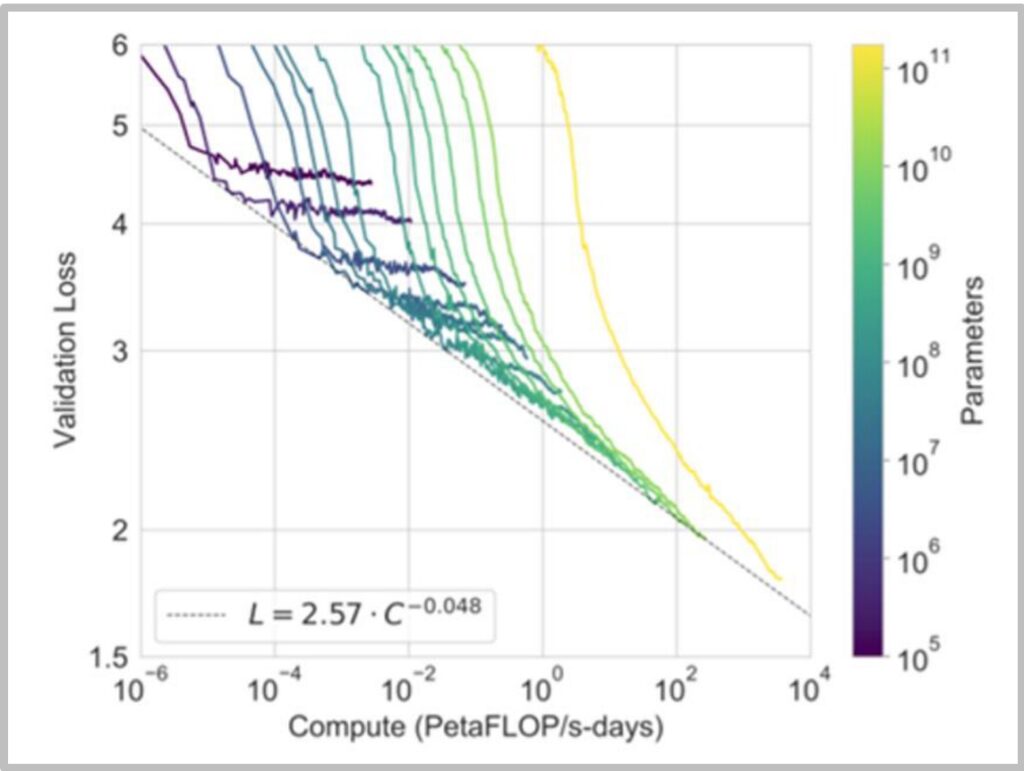
In today’s NLP landscape, we must teach scaling laws because we know that having more compute is fundamentally helpful for training large language models. This scaling relationship holds true whether we’re looking at pre-training or inference scenarios. It’s generally agreed upon that more compute enables more processing of your data, allows you to ingest larger datasets, and supports training of bigger models – all of which lead to improved performance.
Often times, compute leads to predictable performance gains for language models, following well-established mathematical relationships. The relationship follows a power law: \(L = 2.57 \cdot C^{-0.048}\) where \(L\) is loss and \(C\) is compute.
While deep learning algorithms are certainly important, what’s really driven performance improvements is the combination of faster hardware, better utilization, and improved parallelization. For now, these hardware advances alone can drive significant progress in our field. This understanding of compute scaling provides the crucial context for why we need to master GPU optimization – it’s not just about the algorithms we design, but how effectively we can execute them on the available computational resources.
2. Historical Context of Parallel Computing
Evolution from Dennard Scaling to GPU Scaling
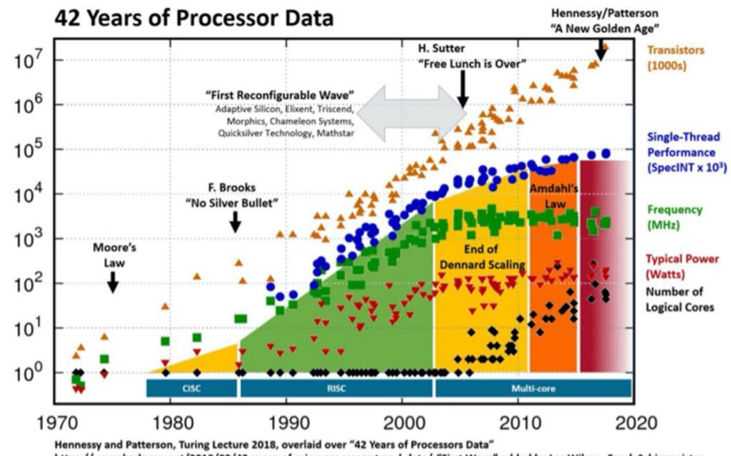
To understand the historical context of parallel computing and why it’s become so crucial for modern AI, we need to look at the evolution of processor performance. When we think about compute scaling and how to make our models train faster, it’s helpful to understand this historical evolution. In the early days of semiconductor scaling, CPUs got faster through something called Dennard scaling. With Moore’s law driving the doubling of transistors on a chip every year, smaller and smaller transistors could be driven at faster and faster clock speeds with lower and lower power consumption, which in turn delivered more performance. This was the golden age of single-thread scaling, where computations could simply be done faster in absolute terms.
🔴 The End of Single-Thread Scaling
However, this approach tapped out between the 1980s and 2000s. You can see in this chart by Hennessy and Patterson that single-thread performance – those blue dots – basically started to plateau. Interestingly, the number of transistors didn’t really start falling off, and chips continued to have higher and higher transistor densities, but this wasn’t helpful anymore. It wasn’t giving higher throughput on single threads. This fundamental shift meant that we couldn’t just do computation faster in absolute terms anymore.
The Transition to Parallel Computing
What we had to make up for it with was parallel scaling. So the story of scaling for deep learning and neural networks is fundamentally about this transition from single-thread scaling to parallel scaling, where you have many workloads that are all computed simultaneously. This shift has been absolutely crucial for the success of modern AI systems, as neural network computations are inherently well-suited to parallel execution.
💡 The GPU Scaling Success Story
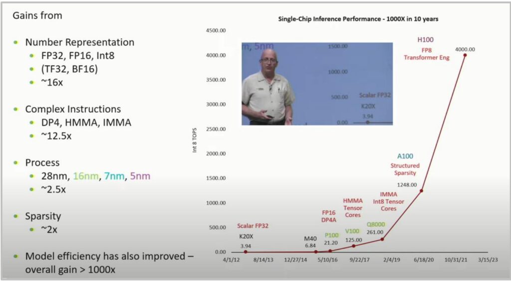
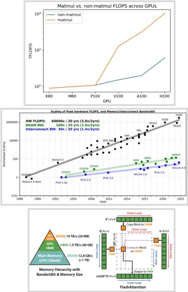
This brings us to one of my favorite computer scaling charts by Bill Dally from his keynote, which shows a super-exponential increase in the number of integer operations per second going from the earliest K20s to the H100. It’s really a remarkable exponential or super-exponential curve that demonstrates the power of parallel scaling with GPUs.
The gains come from multiple factors:
- Number representation (FP32, FP16, Int8, TF32, BF16): \(\sim 16\times\) improvement
- Complex instructions (DP4, HMMA, IMMA): \(\sim 12.5\times\) improvement
- Process technology (28nm to 5nm): \(\sim 2.5\times\) improvement
- Sparsity optimizations: \(\sim 2\times\) improvement
Result: Over 1000× performance improvement in just one decade!
This historical evolution from Dennard scaling to GPU scaling sets the foundation for understanding how we can effectively scale modern language models and neural networks.
3. GPU vs CPU Architecture Comparison
Fundamental Architectural Differences
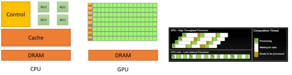
To understand why GPUs excel at parallel computing, we need to start with the fundamental architectural differences between CPUs and GPUs. CPU is something that I think everyone’s familiar with once you start doing programming. It follows this execution model where, in a single-thread, it executes step-by-step what’s happening. To support that kind of execution model, you need big control units that can run these things very quickly because you have a lot of branching and conditional control logic. So the CPU, in this abstracted diagram, dedicates a lot of its chip towards large control branch prediction and runs these very quickly because it doesn’t have that many threads. There are CPUs with lots and lots of cores now, but compared to a GPU, it’s almost nothing.
CPU vs GPU Design Philosophy
In contrast, the GPU has really tons and tons of compute units, ALUs – those little green boxes. There’s much smaller amounts of the chip dedicated to control, so there’s a little bit of control logic orchestrating tons and tons of compute units operating in parallel. If you look at what the design goals are, they are designed for very different objectives:
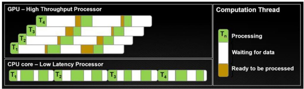
- CPUs optimize for latency: I want to finish my tasks as quickly as possible. If I have tasks \(T_1\) through \(T_4\), in a CPU, I’m going to try to finish each task as quickly as possible, so any one of these tasks will complete really quickly.
- GPUs optimize for throughput: I don’t care about latency – I just want all of my tasks in aggregate to complete as quickly as possible.
In GPU, you’re optimizing for high throughput. I don’t care about latency – I just want all of my tasks in aggregate to complete as quickly as possible. To support that, maybe you have lots of threads, and these threads can go to sleep and wake up very quickly. In the end, you finish all of your workload, \(T_1\) through \(T_4\), before the CPU does, even though individually, all of these have higher latency. You can think of each row as being an SM with its own control units. Each green block might be a FP32 processing unit inside of it, and each SM can operate various pieces that it owns like the tensor cores to do computation.
🔴 Memory is the Real Bottleneck
There are two important things to keep track of when thinking about GPUs. You think of GPU as computers that compute, but actually, computation is only one of the two important things. Memory is arguably more important at this point and will continue to be more important in terms of performance profiles.
To understand memory, you have to understand the physical layout of the GPU and the chip, because when you’re operating at such fast speeds, the physical proximity of the memory starts to matter quite a bit. The closer a piece of memory is to each SM, the faster it’s going to be.
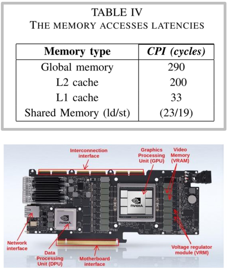
There’s very fast kinds of memory, like L1 and shared memory, that live inside the SM – things like registers that you’re reading and writing very frequently. L2 cache lives in those blue areas right next to the SMs, still on the GPU chip and still pretty fast, though a factor of 10 slower.
💡 The 10× Memory Performance Gap
Outside of the chip itself, you’ve got DRAM living next to the chip that has to physically go outside and connect through those yellow HBM connectors at the edges. The speed differences are dramatic:
- On-SM memory: About 20 clock cycles to access
- L2 cache or global memory: 200 or 300 clock cycles to access
This factor of 10 is going to hurt you real bad. If you have computation that requires accessing global memory, it might mean you actually run out of work to do on your SM. You’ve multiplied all the matrices, run out of work, and now you just have to idle, so utilization won’t be good.
This will be a really key theme – thinking about memory is, in some sense, the key to thinking about how GPUs work. Now let’s dive deeper into the specific components that make up these GPU architectures.
GPU Execution Units and Components
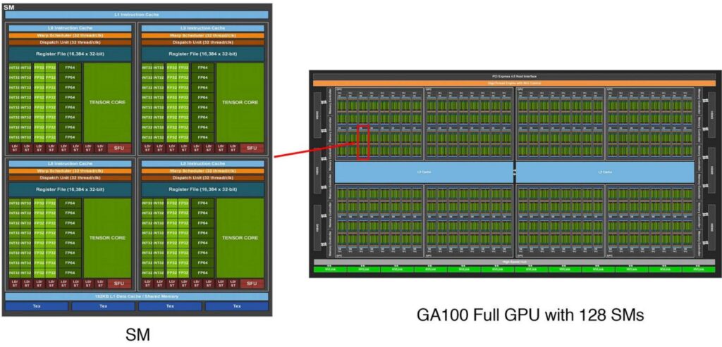
Building on our understanding of GPU’s throughput-oriented design, let’s examine the specific execution units that make this massive parallelism possible. GPUs have a fundamentally different anatomy compared to CPUs, built around a core architectural principle of massive parallelism. The key conceptual foundation of GPU design centers on streaming multiprocessors (SMs) – many independent execution units that serve as the atomic building blocks of GPU computation. When programming with frameworks like Triton, developers operate at the SM level, where each SM functions as a granular unit of control capable of making execution decisions and handling operations like branching. These SMs are designed to independently execute ‘blocks’ or jobs, providing the organizational structure for GPU’s parallel processing capabilities.
The Hierarchical Parallelism Architecture
Within each SM lies another layer of parallelism through streaming processors (SPs), which execute threads in parallel following the Single Instruction, Multiple Data (SIMD) paradigm. While SMs contain the control logic and decision-making capabilities, SPs are optimized for raw computational throughput – they take identical instructions and apply them simultaneously to different pieces of data.
This hierarchical design enables GPUs to perform massive amounts of parallel computation, with each SP handling individual computational tasks while the SM coordinates the overall execution flow.
The scale of this parallel architecture becomes apparent when examining modern GPUs like the A100, which contains 128 SMs – significantly more processing units than even the most advanced multi-core CPUs. Each of these 128 SMs houses a large number of SPs along with specialized matrix multiplication units, creating a computational powerhouse capable of executing thousands of threads concurrently. This massive parallelism is what makes GPUs exceptionally well-suited for workloads that can be decomposed into many independent, similar operations – the foundation of their effectiveness in machine learning and high-performance computing applications. However, to fully understand GPU performance, we need to examine how these execution units interact with the memory system.
GPU Memory Hierarchy Design
As we’ve seen, memory performance is arguably more critical than raw compute power in modern GPU architectures. Understanding GPU memory hierarchy is crucial for optimizing parallel computing performance. The fundamental principle governing this hierarchy is simple yet powerful: the closer the memory is to the Streaming Multiprocessor (SM), the faster it operates. At the innermost level, we have L1 cache and shared memory residing directly inside the SM, providing the fastest access times. Moving outward, L2 cache sits on the GPU die itself, while global memory consists of separate memory chips positioned next to the GPU core.
💡 The Economics of GPU Memory
The performance differences between these memory types are dramatic and directly impact computational efficiency:
- SRAM technology (shared memory/cache): Delivers approximately \(8\times\) faster access speeds compared to DRAM
- DRAM (global memory): Slower but more affordable
- Cost difference: SRAM is roughly \(100\times\) more expensive to manufacture than DRAM
This economic reality drives the hierarchical design, where small amounts of fast SRAM are complemented by larger pools of slower but more affordable DRAM.
The physical layout of modern GPU architectures reflects this memory hierarchy design philosophy. Streaming multiprocessors are strategically distributed across the die, each equipped with its own L1 cache and shared memory resources. Memory controllers and L2 cache partitions are positioned to optimize data flow between the processing units and external memory. This careful spatial organization minimizes latency by reducing the physical distance data must travel, while the hierarchical structure ensures that frequently accessed data can be kept in the fastest available memory tier.
4. GPU Execution and Memory Models
GPU Execution Model Details
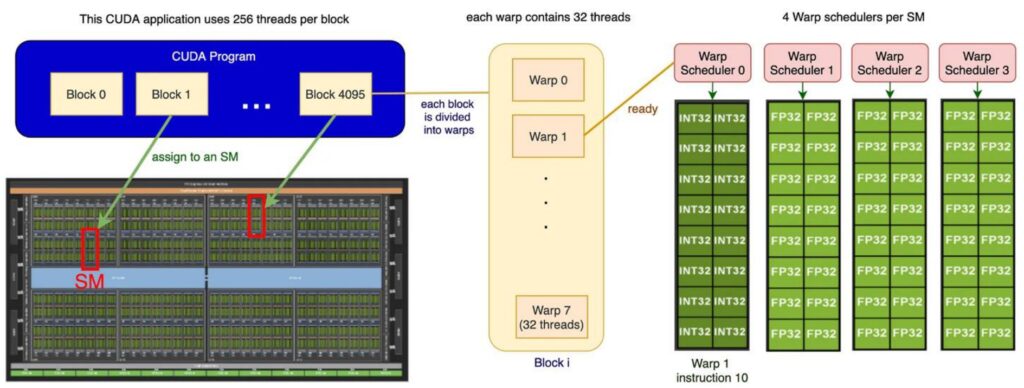
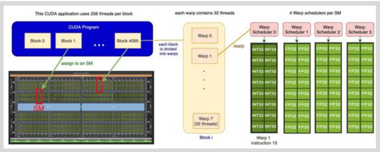
To write high-performance GPU code for assignment two, you need to understand the execution model of how GPUs actually work. There are three important players in the GPU execution model that operate at different granularities: blocks, warps, and threads. This hierarchy narrows down in scope, with blocks being the largest organizational unit consisting of big groups of threads. Each block gets assigned to a streaming multiprocessor (SM), and you can think of each SM as an autonomous worker unit that processes its assigned block independently.
The Three-Level Execution Hierarchy
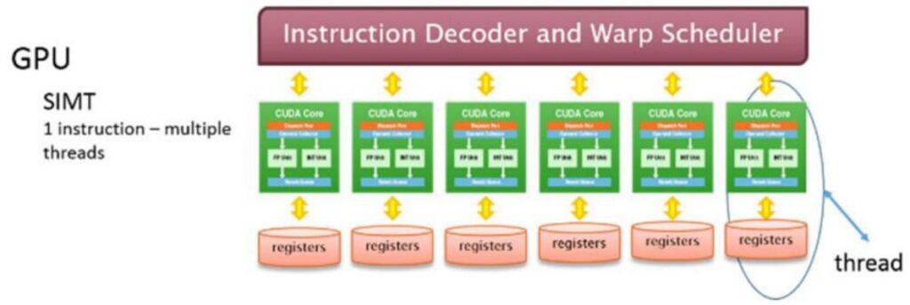
Within each block, you have a collection of threads that represent the actual work units – these threads ‘do the work’ in parallel using a model called SIMT (Single Instruction, Multiple Thread). All threads execute the same instructions but operate on different input data.
However, threads don’t execute individually; instead, they execute in groups called warps. Each warp consists of exactly 32 consecutively numbered threads that execute together as a unit.
So the complete picture looks like this: you have multiple blocks distributed across different SMs, and within each block, there are many different warps. Each SM has its own shared memory that the block can utilize, and the warp schedulers manage how these groups of 32 threads execute their instructions. All threads within a warp execute the same instruction simultaneously but on different pieces of data, which is the essence of the GPU’s parallel execution model.
🔴 Critical Design Implication
Understanding this three-level hierarchy is crucial – threads within warps, warps within blocks, and blocks distributed across SMs – because it has important implications for performance and how we design CUDA kernels.
The way you organize your data and structure your parallel algorithms needs to align with this execution model to achieve optimal GPU performance, which brings us to the equally important topic of how memory is organized and accessed in this execution environment.
GPU Memory Model Architecture
Now that we understand how GPU execution is organized, let’s explore the GPU’s logical memory model – not the physical hardware itself, but rather how you conceptualize GPU programming from a memory perspective. The GPU memory hierarchy consists of several distinct levels, each with different performance characteristics and access patterns. At the fastest level, we have registers for storing individual values, followed by local memory, then shared memory, and finally global memory. As we move up this hierarchy, memory access becomes progressively slower, creating a critical performance consideration for GPU programming.
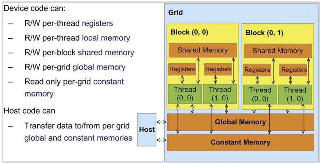
Memory Access Rules and Patterns
The access patterns within this memory hierarchy follow specific rules that directly impact performance:
- Thread-level access: Each thread can access its own registers and the shared memory within its block
- Block-level sharing: Your code can write to global memory and occasionally to constant memory (though the latter isn’t used frequently)
- Cross-block communication: Crucially, any information that needs to be shared across different blocks must be written to and read from global memory, which represents the slowest tier in the hierarchy
💡 The Golden Rule of GPU Memory Programming
This memory architecture has profound implications for optimal GPU programming strategies. The ideal execution model involves loading a small amount of data into shared memory, where all threads within a block can access it quickly and efficiently. This creates a scenario where threads operate on the same localized dataset, maximizing performance through fast shared memory access.
Conversely, if your threads need to access data scattered across different memory locations, they’ll be forced to use global memory access patterns, which are significantly slower and can severely impact performance.
Understanding both the execution model and memory hierarchy gives you the foundation needed to write efficient CUDA kernels that leverage the GPU’s parallel architecture effectively.
6. Performance Optimization Foundations
ML Performance Analysis with Roofline Model
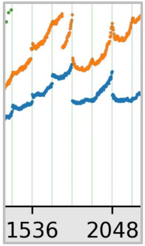
To build a solid foundation for GPU optimization, we need to start by understanding the complex performance characteristics that emerge when running machine learning workloads. Let’s begin by examining what happens when we multiply square matrices together – a fundamental operation in ML. As we look at performance data, the \(x\)-axis represents the size of our square matrix multiplications, while the \(y\)-axis shows the number of operations per second, which we can think of as hardware utilization. As matrices get bigger, we achieve better hardware utilization because we have more work to do, which overwhelms the overhead of launching jobs and similar tasks.
💡 The Performance Mystery
However, there are many strange phenomena happening in these performance curves. You’ll notice multiple different lines that are wavy in unpredictable ways – this behavior might seem chaotic, but it’s actually a natural characteristic of GPU performance. By understanding these patterns, we can make sense of what initially appears to be erratic behavior and learn to optimize our machine learning workloads accordingly.
The overall shape of these performance curves follows what’s known as the Roofline model, a fundamental concept from computer systems. This model reveals that there are essentially two performance regimes when looking at throughput or utilization. On the left side of the curve, we have a memory-limited regime where our computation is constrained by memory bandwidth. On the right side, we enter a compute-limited regime where we’re fully utilizing our compute units – all the matrix multiply units are working continuously.
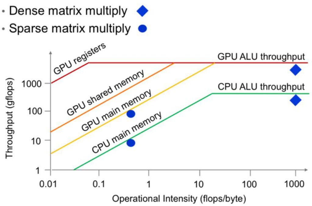
Understanding the Roofline Model
The diagonal portion of the roofline represents the memory-bound region where our performance is limited by memory bottlenecks rather than computational intensity. Our goal is to avoid being stuck in this left-side region and instead operate in the right-side regime where we achieve full utilization of all compute units.
The ideal roofline model shows this characteristic shape: a diagonal part transitioning into a flat plateau at the top, representing maximum computational throughput. This theoretical framework gives us the foundation we need to understand specific optimization strategies.
GPU Optimization Strategy Overview
Building on our understanding of the roofline model, let’s dive into the practical side of GPU optimization. While the fundamental principle is straightforward – minimize unnecessary memory accesses, particularly to slow global memory – achieving this requires mastering a large array of optimization tricks, as there are many pitfalls that can severely impact performance. We’ll explore six core areas critical to GPU performance: control divergence (which isn’t actually a memory bottleneck), low precision computation, operator fusion, recomputation, coalescing memory, and tiling.
🔴 Control Divergence: The SIMT Penalty
The first critical issue to understand is control divergence, which stems from GPU’s SIMT (Single Instruction Multi-Thread) execution model. In this architecture, every thread within a warp must execute the same instruction simultaneously, operating on different data. This creates serious performance problems when we introduce conditional statements within a warp.
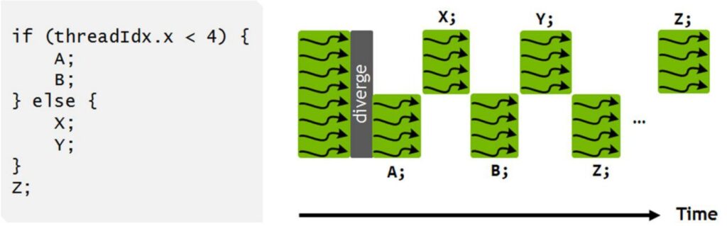
Consider this simple conditional code example:
if (threadIdx.x < 4) {
    A;
    B;
} else {
    X;
    Y;
}
Z;
When executed on a GPU, the hardware cannot run both branches simultaneously. Instead, it first executes the ‘A’ and ‘B’ instructions on the four threads where \(threadIdx.x < 4\), while pausing the remaining threads. Then those paused threads wake up to execute the ‘X’ and ‘Y’ instructions while the original four threads go idle. This serialized execution of divergent control paths within a single warp can be extremely damaging to performance, as it forces threads that should be running in parallel to instead wait for each other.
7. Low Precision Computation Optimization
Low Precision Benefits and Implementation
Moving beyond the obvious advice about avoiding conditionals in massively parallel compute units, we need to focus on memory-based optimization tricks. The first and most important technique I want to discuss is lower precision arithmetic – this is a big trick that you should implement all the time. When you look at the impressive performance gains shown in GPU development over the years, the numbers keep climbing exponentially, which looks fantastic on paper.
The Secret Behind GPU Performance Gains
However, when you dig deeper into what’s actually driving this GPU progress over all these years, you discover that it’s fundamentally about number representations. The evolution from FP32 to FP16 to Int8 and beyond has delivered many orders of magnitude gains simply by using lower and lower precision in GPU operations. This progression represents one of the most significant factors behind the dramatic performance improvements we’ve witnessed.
💡 Memory Efficiency Through Lower Precision
The beauty of lower precision lies in its direct impact on memory efficiency. When you have fewer bits in all the computations, weights, and data structures you’re working with, you dramatically reduce the number of bits that need to be moved around.
Even when you’re accessing these bits from global memory – typically the most expensive memory operation – they become much less of a performance concern because there’s simply less data to transfer. This memory efficiency becomes particularly important when we consider how arithmetic intensity affects different types of operations.
Arithmetic Intensity and Matrix Multiplication Improvements
Building on the memory efficiency benefits we just discussed, let’s explore arithmetic intensity through a simple example of an element-wise operation. Consider implementing ReLU (\(x = \max(0, x)\)) on a vector of size \(n\) using float32 precision. For memory accesses, we need to read \(x\) and write the result if \(x < 0\), which totals 8 bytes in float32. The operations involve one comparison (\(x < 0\)) and one FLOP, giving us an arithmetic intensity of 8 bytes per FLOP. However, if we switch to float16 precision, we haven’t changed the FLOP count, but we’ve halved the memory access to 4 bytes per FLOP. In essence, we’ve doubled our effective memory bandwidth for free, assuming we can work with float16 precision.
Mixed Precision in Matrix Multiplication
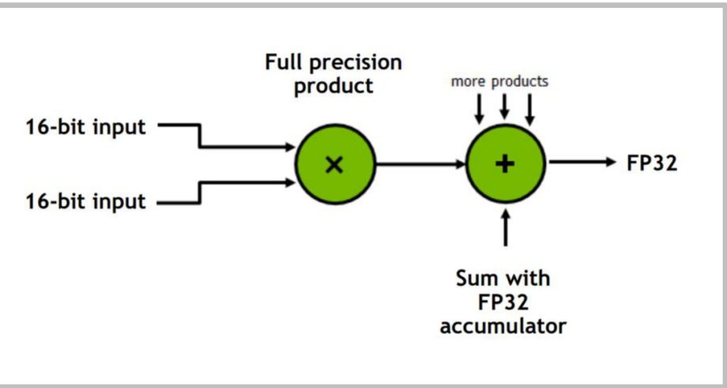
This principle of mixed precision becomes particularly important in matrix multiplications. The strategy involves:
- Storing inputs in 16-bit precision for memory efficiency
- Performing the actual multiplication and accumulation in full 32-bit precision
- Returning an FP32 result, which can then be downcast back to 16-bit if desired for storage
This approach is crucial because intermediate computations, especially when accumulating partial sums, benefit from higher precision to avoid rounding errors that can occur when adding small values to large sums.
🔴 When NOT to Use Low Precision
However, not all operations in your network should use low precision. While matrix multiplications and most pointwise operations like ReLU, tanh, add, subtract, and multiply can often work well with 16-bit storage, other operations require more careful consideration:
- Reduction operations such as sum, softmax, and normalization typically need higher precision due to their accumulative nature
- Pointwise operations where \(|f(x)| \gg |x|\) (like exp, log, pow) and loss functions often require more dynamic range and precision
- Operations that lack sufficient dynamic range might blow up or zero out, making BF16 a better choice for its extended range compared to FP16
💡 The Engineering Challenge
The engineering challenge lies in carefully balancing precision requirements across different parts of your network and training algorithm. When done correctly, mixed precision training can effectively double your throughput by moving from 32 to 16-bit precision, especially when memory bandwidth is your bottleneck.
This requires thoughtful consideration of which operations can safely use lower precision while maintaining model stability and training convergence.
8. Operator Fusion Techniques
Fusion for Memory Access Optimization
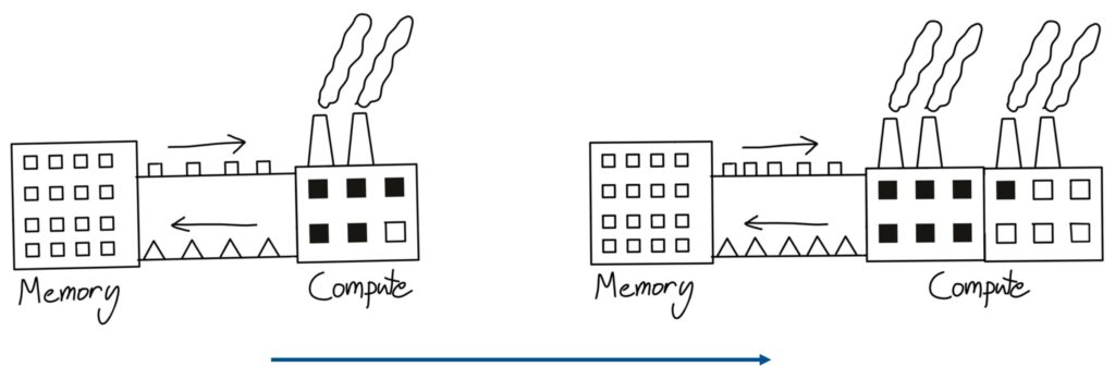
When people think about writing CUDA kernels, operator fusion is both intuitive and naturally appealing to consider. One useful mental model for understanding how GPUs and memory work comes from this factory analogy. Imagine you have a factory that represents your compute unit – it takes in little box widgets and outputs triangle widgets. If you scale up your compute capacity by adding more factories, but your conveyor belt that transfers memory to compute has finite bandwidth, you won’t be able to utilize that second factory effectively. You’re still bottlenecked by the speed at which you can transfer data from memory to compute.
💡 The Naive Computation Pattern
One insidious way you can incur tremendous overhead without realizing it follows this naive computation pattern. Picture the left side as your memory and the right side as your compute unit. To perform computation, you start with squares and move them from memory to compute, do some operation to turn them into triangles, then shift the triangles back to memory. When you realize you need those triangles again, you shift them back to the compute unit where triangles become circles, and so on.
This back-and-forth data movement between compute and memory represents a very naive approach that incurs tons of memory overhead.
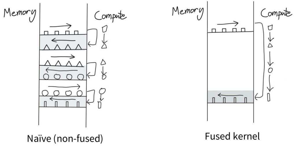
The Fused Kernel Mental Model
The key insight is recognizing that when there are no dependencies between operations, you should be able to go from square to triangle to circle to rectangle and only then ship the final result back to memory. You can keep everything in the compute unit the entire time, avoiding the constant back-and-forth transfers.
This represents the mental model of a fused kernel – when you have multiple operations that need to happen on a piece of data in sequence, instead of writing intermediate results back to storage after each step, you perform as much computation as possible in one place and only ship the final result back to memory when necessary.
This concept becomes especially important when you need to perform many operations in sequence. The naive approach of shipping data back and forth between memory and compute for each individual operation is frankly quite silly from an efficiency standpoint. Kernel fusion addresses this by consolidating multiple operations into a single execution unit, dramatically reducing memory access overhead and improving overall performance. Now let’s see how this plays out in practice with some concrete examples.
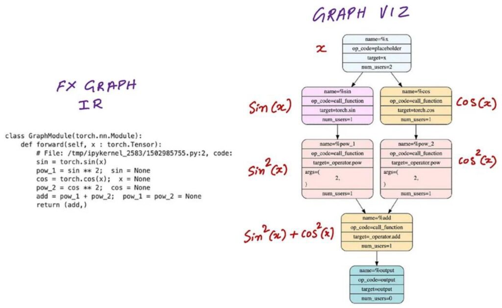
Practical Fusion Examples and CUDA Optimization
Building on our theoretical understanding, let’s explore some very simple examples of how naive code can lead to inefficient CUDA kernel launches. Consider writing a neural network module that takes input \(x\) and produces \(\sin^2(x)\) and \(\cos^2(x)\). When you run this in PyTorch, the computation graph will launch a whole bunch of separate CUDA kernels – one to compute \(\sin(x)\), another for \(\cos(x)\), then separate kernels for \(\sin^2(x)\) and \(\cos^2(x)\), and finally one more for the addition \(\sin^2(x) + \cos^2(x)\). This creates a lot of back-and-forth communication between GPU memory and compute units, exactly like the inefficient pattern we discussed earlier.
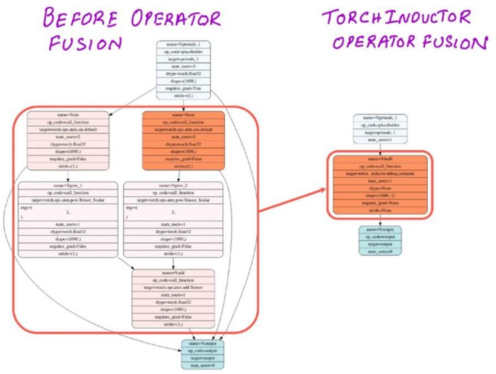
Smart Operator Fusion
However, if you’re a bit smarter about this – either by writing your own CUDA kernel or using something like Torch Compile – you can easily realize that those five operations don’t really depend on very much external memory. They use only a small amount of local memory, which means you can fuse them into a single operation that does everything on the GPU within a single thread block without constantly sending intermediate results back to global memory.
This kind of operator fusion transforms what would be five separate kernel launches into just one optimized kernel call.
💡 Automatic Fusion with Modern Compilers
The great news is that really easy fusion operations like this can be done automatically by modern compilers. I just mentioned Torch Compile, and if you aren’t already using this feature, you should strongly consider incorporating Torch Compile everywhere in your code.
These ‘easy’ fusions involving pointwise operations are exactly the kind of optimizations that compilers excel at, and we’ll be showing you how to use Torch Compile effectively in the upcoming assignment as well.
9. Memory Management Strategies
Recomputation for Memory Optimization
Moving beyond precision and fusion techniques, another powerful optimization strategy we can employ on GPUs is called recomputation. This approach involves spending additional compute cycles to avoid costly memory access operations. The basic idea works like this: we start with our inputs at the bottom (shown as yellow values), propagate activations upward through the computational tree, then compute the Jacobians backward (represented as green values on the edges). To calculate gradients, we multiply the Jacobians with the activations and propagate the gradients backward through the network.
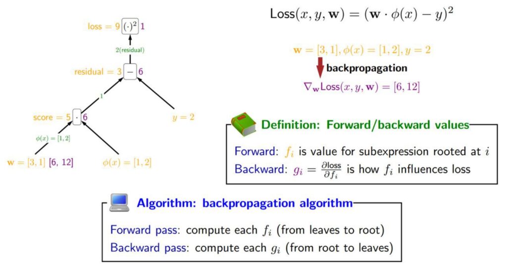
🔴 The Traditional Backpropagation Bottleneck
The challenge with traditional backpropagation is that those yellow activation values from the forward pass must be stored in global memory, then retrieved and loaded into compute units during the backward pass. This creates a significant amount of memory input and output operations that can become a performance bottleneck.
However, recomputation offers an elegant solution to avoid this memory overhead by trading compute for memory bandwidth.
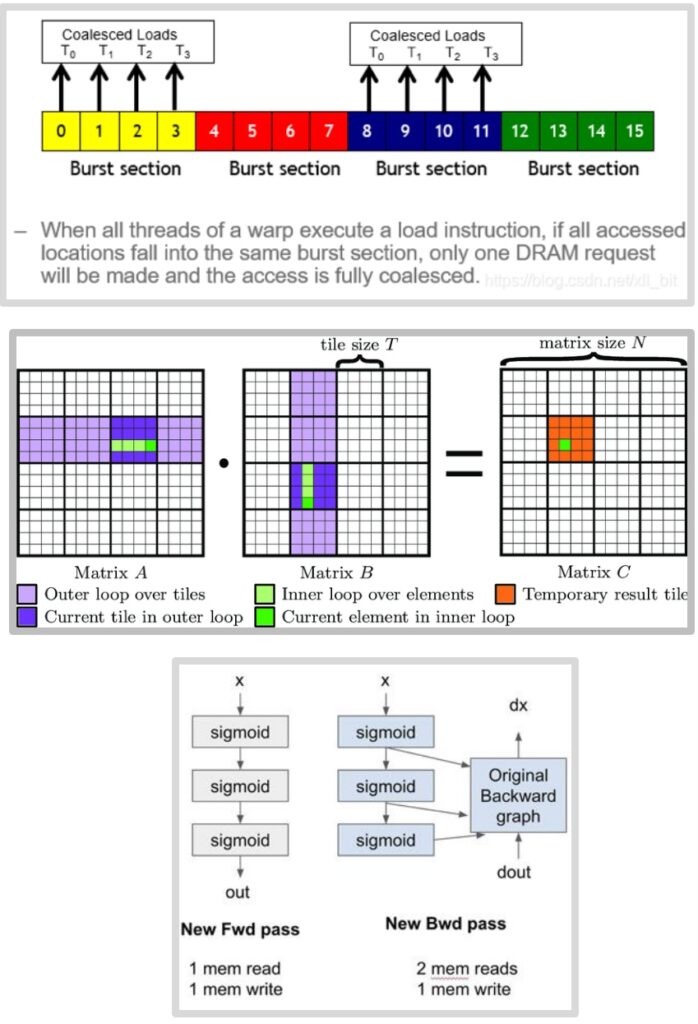
Let me illustrate this with a concrete example: imagine we stack three sigmoid activation functions on top of each other. The forward graph shows the sequential computation through each sigmoid layer. In the traditional approach, we compute the sigmoids and store the intermediate activations \(S_1\) and \(S_2\), along with our final outputs. During the forward pass, we perform one memory read of \(x\) and three memory writes for \(S_1\), \(S_2\), and the output.
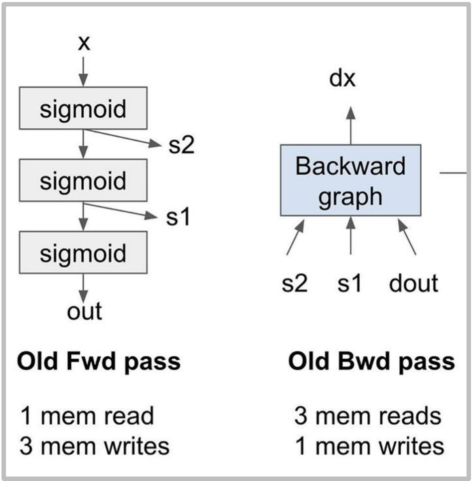
The Memory Access Problem
The backward pass becomes particularly problematic in this scenario. We need to retrieve the stored values \(S_1\) and \(S_2\) from memory, combine them with the gradients flowing backward, and push the results through the backward computation to obtain the gradient of \(x\). This requires three memory reads and one memory write for the backward pass alone.
In total, we’re performing eight memory operations with very low arithmetic intensity since there are no matrix multiplications involved. This is really terrible for performance and demonstrates why recomputation can be such a valuable optimization technique.
Activation Recomputation Implementation
So how do we actually implement this recomputation strategy? The core idea is elegantly simple: instead of storing intermediate activations in memory, we throw them away and recompute them on the fly during the backward pass. In this new approach, the forward pass takes \(X\) as input, computes the sigmoid operations, and produces the output without storing intermediate values like \(S_1\) and \(S_2\). This results in just one memory read for \(X\) and one memory write for the output, dramatically reducing our memory footprint.
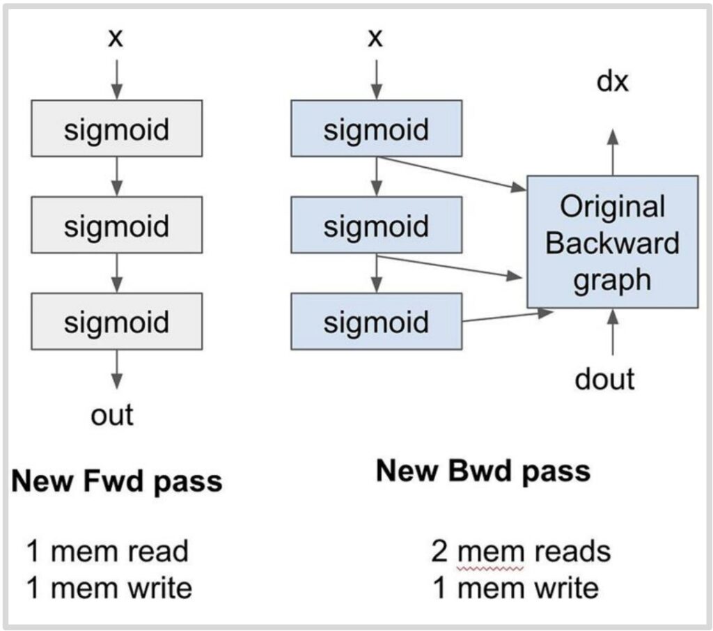
💡 The Recomputation Magic
During the backward pass, since we no longer have stored activations, we need both the gradient signal \(D_{out}\) coming from above and the original input \(X\) – that’s two memory reads. The magic happens in the streaming multiprocessor’s local memory, where we recompute \(S_1\), \(S_2\), and the output on the fly, feeding them directly into the backward computation graph.
Because this recomputation happens entirely in local memory, there are no additional global memory reads, and we only have one final memory write for \(D_X\).
The Striking Results
The results are striking: we achieve \(5/8\) of the memory accesses for the exact same computation. Yes, we pay the price of recomputing those three sigmoid operations, but here’s the beautiful insight – if you were already running idle because you were memory-bound, this becomes a fantastic trade-off. You’re essentially trading excess compute capacity, which you had too much of, for memory bandwidth, which was your bottleneck.
This technique shares DNA with gradient checkpointing and activation recomputation for memory savings, but the motivation is fundamentally different. While traditional checkpointing is about surviving when you’re running out of memory, this recomputation strategy is about execution speed optimization. It’s the same core technique applied to different goals – a perfect example of how throwing away computation can actually be optimal when it unlocks better resource utilization. This completes our exploration of memory management strategies, showing how clever trade-offs between compute and memory can lead to significant performance gains.
10. Memory Access Pattern Optimization
Memory Coalescing Fundamentals
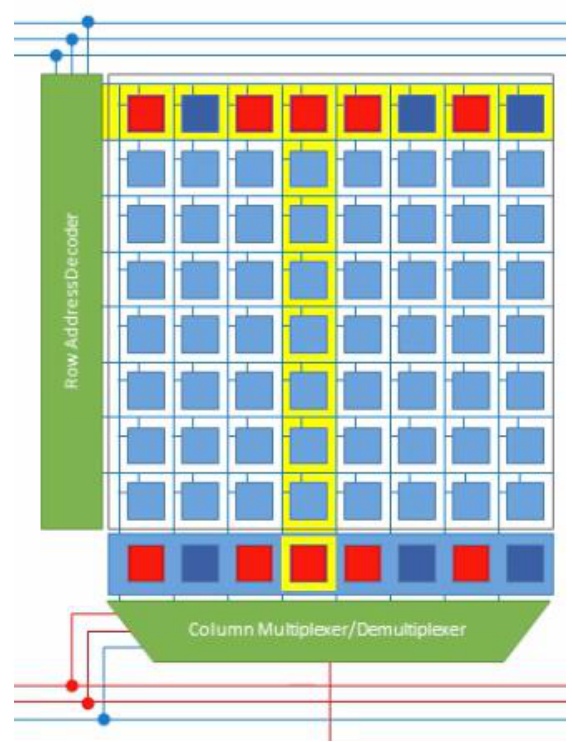
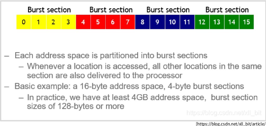
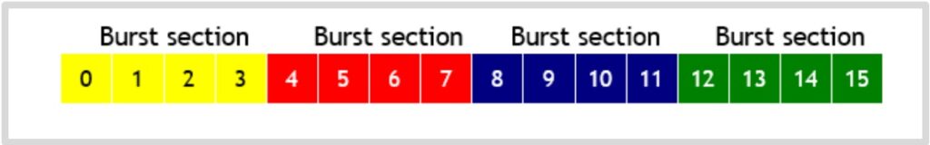
To truly optimize memory access patterns, we need to understand how GPU memory systems work at the hardware level. Here’s something really fascinating that I didn’t know until I started diving deep into how GPU hardware and DRAM actually work. The slow memory – what we call global memory or DRAM in a GPU – is incredibly slow. But there are clever hardware-level optimizations designed to make it faster, and one of the most important is called burst mode. When you request a single piece of memory, you don’t just get that one value back. Instead, the memory system gives you a whole chunk of contiguous memory. So if I tried to read the very first value from a memory block, instead of just getting that single byte, the system would actually return four values at once – giving me the requested byte plus three additional ones it assumes I’ll probably need soon.
Why Burst Mode Exists
Why would memory give you three extra bytes for free when you only asked for one? There’s a fascinating hardware reason behind this. When you’re addressing memory, the expensive step is moving the data from storage to the amplifier – that’s what takes time. But once you’ve done that costly operation, you can grab many additional bytes essentially for free.
The entire address space gets divided into these burst sections, and you receive the complete section rather than just your specific request.
💡 The Throughput Opportunity
This creates an opportunity to dramatically accelerate memory access if your access pattern is smart. If you access memory randomly, you’ll need roughly as many queries as the length of your data. But if you access the first value of a burst section, you get the entire section at once. Then when you access the first value of the next burst section, you get that entire section too.
This means you can potentially achieve four times the throughput if you’re clever about only accessing the bits you need from each burst section.
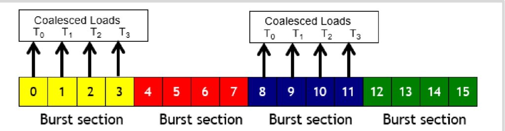
This optimization is called memory coalescing, and it’s particularly powerful in GPU computing. Remember that a warp consists of 32 numbered threads, and memory accesses from a warp happen together. When all threads in a warp execute a load instruction and all their accessed locations fall within the same burst section, the smart hardware groups those queries together. Instead of making separate requests for threads \(T_0\), \(T_1\), \(T_2\), and \(T_3\), it makes just one request and delivers all the data at once through burst mode DRAM. When memory accesses are fully coalesced like this – meaning all threads fall within the same burst section – you can achieve a 4× improvement in memory throughput. Now let’s see how these coalescing principles apply to one of the most important operations in neural networks.
Coalescing in Matrix Multiplication
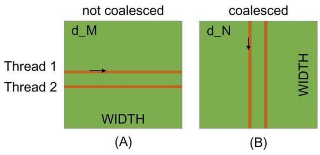
When implementing neural networks from scratch in CUDA, understanding memory coalescing in matrix multiplication becomes absolutely critical. There are fundamentally two ways to read matrices: you can traverse by rows, where each thread goes across a row, or you can read in column order, where each thread moves down a column. The choice between these approaches has dramatic performance implications that many developers overlook.
🔴 The Performance Trap
The left approach, where each thread accesses different rows and goes through columns, turns out to be quite slow because the memory reads are not coalesced. In contrast, the right side approach, where threads increment down rows, enables coalesced memory reads.
For row-major matrices, threads that move along rows are not coalesced, which creates significant performance bottlenecks that can cripple your implementation.
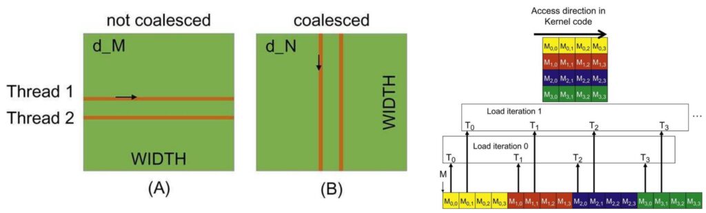
To understand why this happens, consider what occurs at each time step. In the non-coalesced approach, at time step 1, the first thread loads one point, the second thread loads a completely different point, and so on. These threads end up reading from different burst sections, which means you have to read entire chunks of memory just to perform simple operations. This is incredibly inefficient and wasteful.
The Correct Approach: Column-Wise Access
However, when you go in the column direction, all threads read within a single burst section, meaning only one memory read operation needs to be performed and you get all the memory at once. Note how the second diagram reads the entire vector at each step!
This is a very low-level optimization, but it’s incredibly important. If your memory traversal order is wrong, you’ll get much slower memory accesses than you want, and your neural network implementation will suffer dramatically. Understanding these coalescing patterns is essential for writing high-performance CUDA kernels.
11. Advanced Tiling Optimization
Tiling Concepts and Shared Memory Usage
Now we come to the very last and perhaps most important optimization concept: tiling. Tiling is the idea of grouping together memory accesses to minimize the amount of global memory access we have to do. To explain this, let me walk through a matrix multiply example that will hopefully show you why a naive algorithm for matrix multiplication is very problematic, and then demonstrate how a tiled version reduces the number of global memory reads required.
🔴 The Naive Matrix Multiply Problem
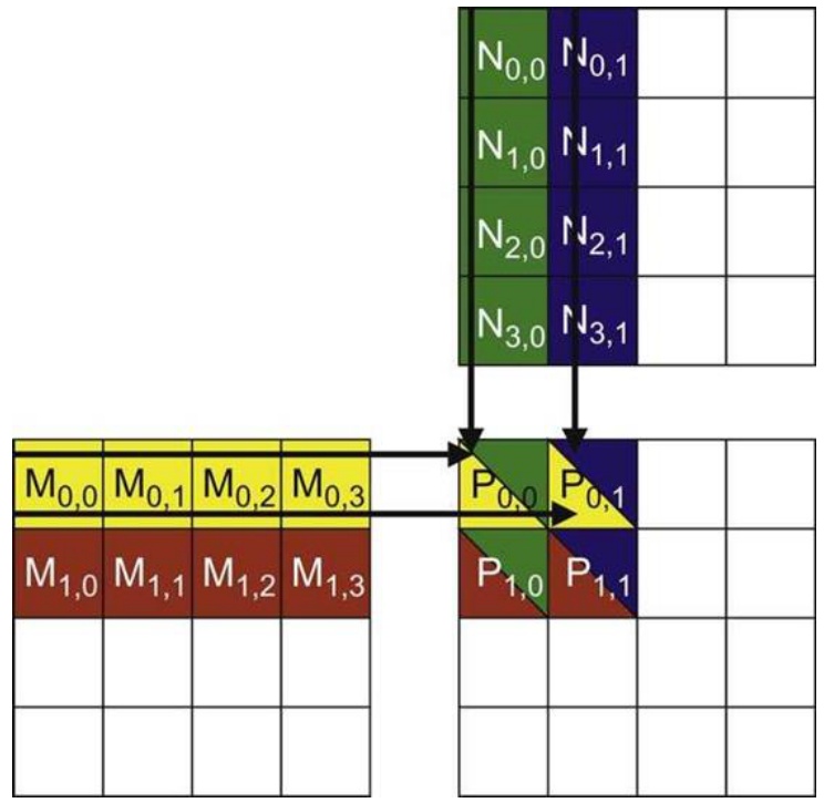
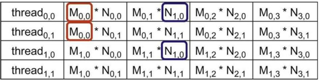
Let’s start with a simple matrix multiply algorithm. I have an \(M\) matrix on the left and an \(N\) matrix on the top. To compute the matrix-matrix product, I need to traverse over the rows of \(M\) and the columns of \(N\), take their inner product, and store that into the corresponding position in the \(P\) matrix.
Each thread (thread\(_{0,0}\), thread\(_{0,1}\), thread\(_{1,0}\), thread\(_{1,1}\)) accesses elements in a specific order to compute their assigned output. Notice that the memory access here is not coalesced – the row matrices are accessed in a non-coalesced order. More importantly, I have repeated memory accesses: \(M_{0,0}\) is accessed by multiple threads, and \(N_{1,0}\) is accessed by different threads. These values are being read over and over from global memory into many different threads, making this potentially very slow.
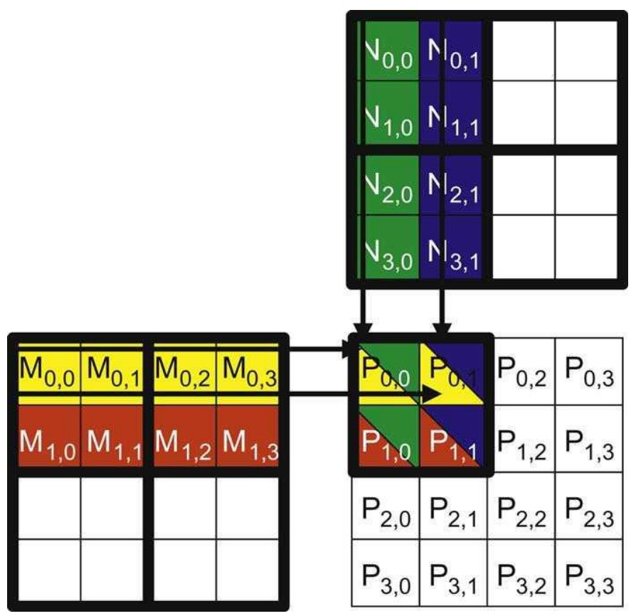
The question becomes: can we avoid having too many global memory reads and writes? The ideal outcome would be to spend one chunk of time loading pieces from global memory to shared memory where things are fast, do a ton of computation in shared memory, and then be done with that piece of data – minimizing global memory accesses. Here’s how we can achieve this in matrix multiplication: I’m going to take both the \(M\) matrix and the \(N\) matrix and cut them up into tiles. In this example, I’ve created 2×2 tiles, giving me smaller sub-matrices within each matrix. If my shared memory is big enough to fit these sub-matrices within each SM, this gives us a very simple and efficient algorithm.
The Tiled Algorithm
The tiled algorithm works as follows: First, I load the \(M_{0,0}\) and \(N_{0,0}\) tiles into shared memory. Now I can compute partial sums by taking the row products and incrementing them into \(P_{0,0}\). I can do the same with all the different sub-matrices that I can process with these loaded tiles.
Once I’m completely done processing these two tiles, I can load new tiles – say \(M_{0,0}\) and \(N_{2,0}\) – into shared memory and repeat the computation, incrementing my partial sums in \(P\). This approach has really consolidated and reduced the amount of global memory access I need to do.
Mathematical Foundations of Tiling
Let me show you mathematically why this tiling approach is so powerful and delivers such dramatic performance improvements. The key to understanding tiling’s effectiveness lies in carefully tracking where data is being read from – whether from fast shared memory or slow global memory.
💡 The Mathematics of Memory Reduction
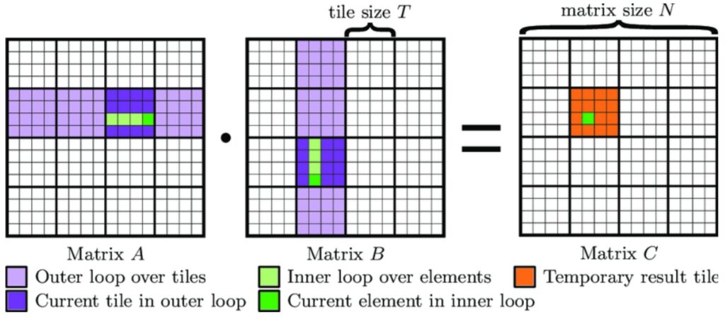
The mathematics of tiling reveals a powerful optimization opportunity. In a non-tiled matrix multiply, where we simply iterate over rows and columns, every input element must be read from global memory each time it’s processed. This means each input is read approximately \(n\) times from global memory throughout the entire computation. However, with a tiled approach, the global memory reads operate over tiles rather than individual elements.
In the tiled matrix multiply, each input is read only \(\frac{n}{t}\) times from global memory, while being read \(t\) times within each tile from the much faster shared memory. We can’t reduce the total number of reads – we still need to access all matrix elements – but we can strategically shift these reads from slow global memory to fast shared memory. This results in \(t\) times memory reads into shared memory and \(\frac{n}{t}\) times from global memory, giving us a factor of \(t\) reduction in the total amount of data that must come from global memory.
This tiling strategy becomes incredibly powerful when working with matrices, especially when we have substantial shared memory that can accommodate large tiles. The larger our tile size \(t\), the greater the reduction in global memory access, making tiling one of the most effective optimization techniques for matrix operations. However, as we’ll see next, implementing tiling effectively comes with its own set of complex challenges that can make or break your performance gains.
Tiling Implementation Challenges
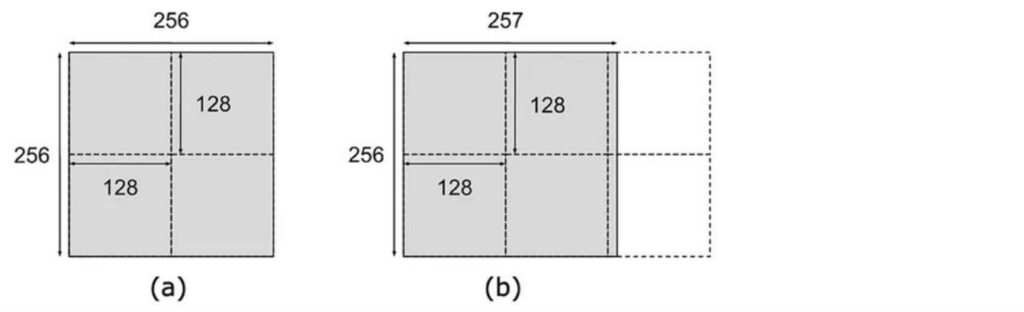
While the mathematical benefits of tiling are clear, the practical implementation is quite complex and serves as the source of many confusing aspects about GPU and matrix multiply performance. The challenge begins with discretization – imagine having a tile size of \(128 \times 128\), which seems like a nice, round tile size. When you have a matrix of size \(256 \times 256\), that’s perfect – you get a clean \(2 \times 2\) tiling pattern and things load nicely. However, problems arise when dimensions don’t align well. For instance, if you have a matrix that’s \(256\) on one dimension but requires six tiles to cover completely, the two tiles on the right become very sparse with minimal data. This creates a serious performance bottleneck because each tile gets assigned to a streaming multiprocessor (SM), and those underutilized tiles leave their corresponding SMs sitting idle when you’d prefer to distribute the computational load evenly across all available resources.
🔴 The Balancing Act
Optimizing tile sizes requires balancing multiple competing constraints. You need to:
- Ensure coalesced memory access patterns
- Stay within shared memory size limits
- Achieve divisibility of the matrix dimensions to avoid the underutilized SM scenario
The tiles can’t be too large or they’ll exceed your shared memory capacity, but they need to divide the matrix dimensions as evenly as possible. While GPUs naturally overlap memory reads and computation to utilize available bandwidth, the reality is that when you’re effectively utilizing your SMs, you’re typically maxed out on shared memory – that’s the bottleneck resource. This leaves no room for prefetching, creating additional performance considerations.
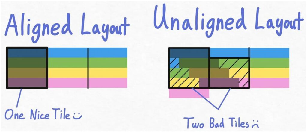
The interaction between tiling and burst sections adds another layer of complexity. In an ideal scenario, your matrix layout aligns perfectly with burst sections, where each burst section lines up nicely with a tile boundary. To read such a tile, you only need to fetch four different burst sections to get the entire tile efficiently. However, adding even a single extra element can completely disrupt this alignment. When burst sections flow over due to misalignment, loading a tile becomes much more expensive – the first row might load as a complete burst section, but subsequent rows may span two different burst sections, requiring double the memory reads. This misalignment can easily double your memory access requirements simply because the rows don’t line up with burst section boundaries.
💡 The Solution: Strategic Padding
The solution to these alignment issues involves strategic padding to achieve nice, round matrix sizes that ensure burst sections align properly with tile dimensions. If your matrix sizes aren’t multiples of your burst section size, you’ll inevitably encounter these performance-killing scenarios.
While this might seem like a minor detail, these considerations become critical when you want to squeeze out maximum performance from your matrix multiplications. These are exactly the kinds of subtle issues that will bite you if you’re not thinking about them upfront, but mastering them is essential for achieving optimal GPU performance.
12. Performance Analysis Case Study
Matrix Performance Mystery Introduction
Let’s dive into a fascinating real-world performance case study that perfectly illustrates the optimization principles we’ve been exploring. Modern optimization frameworks like Torch Compile and CUDA optimizations for matrix multiplies are implementing exactly these kinds of performance techniques we’ve been discussing. This leads to some fascinating real-world examples, like Andre Karpathy’s tweet about nano-GPT optimization. The most dramatic performance boost came from simply increasing the vocabulary size from 50,257 to 50,304 – making it the nearest multiple of 64. This seemingly minor change of adding just 47 dimensions to the vocabulary resulted in a 25% speedup due to much higher GPU occupancy. It’s a perfect illustration of how careful attention to powers of 2 and memory alignment can yield dramatic performance gains.
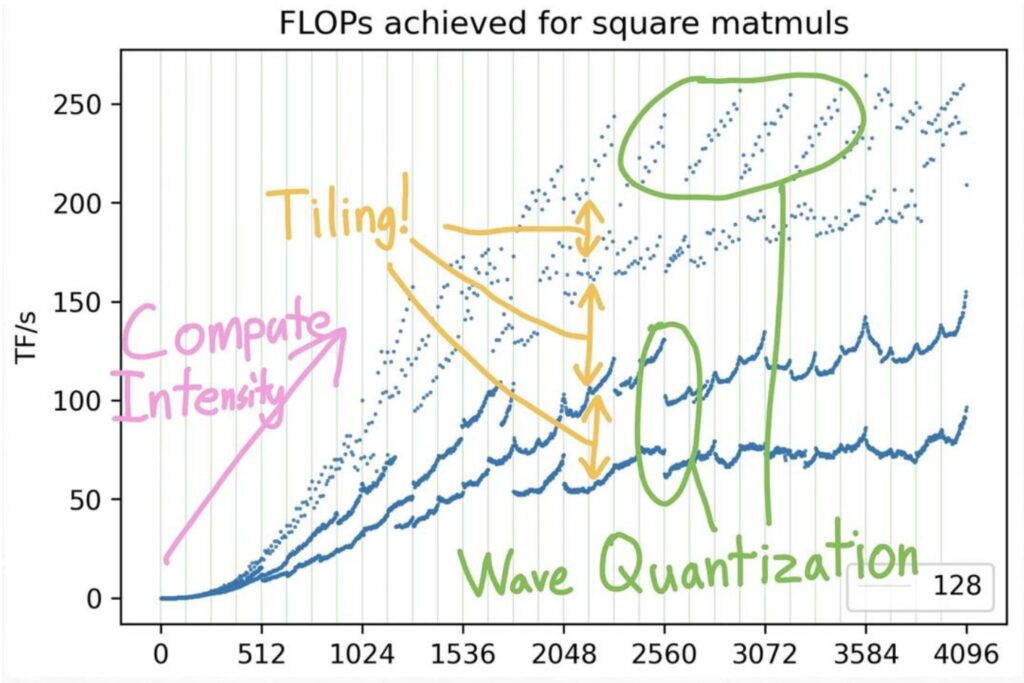
This brings us to the heart of our matrix performance mystery, and now we can finally explain how these complex performance patterns emerge. The concept of compute intensity becomes crucial here – it’s exactly the roofline model we pointed out at the beginning of our discussion.
Understanding the Performance Regions
Looking at this performance chart, we can see distinct regions that explain the mystery. Up until around matrix size 1536, there simply isn’t enough matrix multiply work to keep the GPU busy – just loading the matrix and doing basic I/O operations becomes the bottleneck. Below this point, throughput falls dramatically because you don’t have sufficient memory bandwidth to support your compute units.
On the right side of the chart, we see the theoretical upper envelope representing maximum achievable performance, where it’s possible to saturate all compute units and achieve excellent performance.
However, the real complexity lies in those strange performance valleys and peaks throughout the chart. If you mess up your matrix sizing, you can end up in these peculiar performance troughs, even within regions where good performance should be achievable. The first major factor behind these mysterious patterns is memory alignment – let’s examine how tiling alignment creates these dramatic performance variations.
Memory Alignment Impact Analysis
Building on those performance valleys we just observed, the very first thing we need to understand is this tiling alignment issue. When you look at the multiples here, I’ve colored each of these lines based on the visibility of the matrix, and this represents the size by which it’s divisible. If your matrix is divisible by 32, then you’re in good shape – you’re in these purple dots up here. If you’re divisible by 16, you’re actually still performing well up here, and there are two colors representing this. The green dots indicate your \(k\) equals 8, while orange represents \(k\) equals 2, and if your \(k\) equals 1, you’re all the way down here at the bottom.
🔴 Critical Advice: Avoid Prime Dimensions
Here’s a crucial piece of advice: don’t pick prime dimensions if you want good throughput on your matrix multiplies. If you’re not divisible by any reasonable number, you’re going to suffer performance-wise. A big part of this problem emerges once you get to \(k\) equals 2 and \(k\) equals 1, because you’re basically forcing a situation where you can no longer read tiles in this nicely aligned way with your burst reads. This leads to some serious performance issues that can be quite dramatic.
The performance degradation can be quite shocking – you can see this dramatic drop from high-performance regions all the way down to these bottom points, where you’re left wondering what happened. How could you possibly lose so much performance by simply increasing your dimension by 2? This is the power of alignment issues in memory access patterns, and it’s something that can catch you completely off guard if you’re not aware of these underlying hardware constraints. But memory alignment is just one piece of the puzzle – there’s another equally important phenomenon that creates these performance valleys.
Wave Quantization Effects
Beyond memory alignment issues, there’s another critical factor creating those mysterious performance drops: wave quantization effects. Let’s examine what happens when we look at the performance characteristics within this orange line. If you zoom in closely, you’ll notice a dramatic drop that occurs when transitioning from a matrix size of 1792 to what we’ll call 1792 by 4 (keeping it as a factor of two). For our analysis, let’s consider using a tile size of 256 by 128, which is quite natural since the matrix multiply units in GPUs operate efficiently on matrices of roughly size 128. This makes 256 by 128 an optimal tile configuration.
$\(\frac{1792}{256} \times \frac{1792}{128} = 7 \times 14 = 98\)$
The Tile Count Problem
With our tile dimensions established, we can calculate that there are exactly \(7 \times 14 = 98\) different tiles when dividing our matrix dimensions by the tile sizes. However, when we increase the matrix size by just one dimension, we’re forced to round up each coordinate, dramatically increasing our tile count to 120. This seemingly small change has profound implications for GPU utilization.
$\(8 \times 15 = 120\)$
🔴 The SM Capacity Bottleneck
The problem becomes clear when we consider that an A100 GPU has exactly 108 streaming multiprocessors (SMs), which are the parallel execution units. With 98 tiles, all SMs can run simultaneously, achieving excellent utilization. But once we jump to 120 tiles, we exceed the SM capacity – only 108 tiles execute initially, leaving 12 tiles for a second wave with dramatically reduced utilization.
This phenomenon is called wave quantization, and it creates a characteristic performance pattern: good utilization initially, followed by a dramatic drop-off, then a period of very low utilization as the remaining tiles complete. To avoid this quantization error, it’s ideal to design tile sizes that are either much larger than the number of SMs, or structured so you don’t end up just barely exceeding the SM count and triggering this inefficient second wave of execution. Now that we understand both memory alignment and wave quantization effects, let’s synthesize these insights into practical optimization strategies.
ML Optimization Summary
Having explored memory alignment and wave quantization effects in detail, let’s step back and synthesize the key optimization principles that emerge from this analysis. I know this is low level details, but in many ways, you know, I’ve been saying through many classes that language models and deep learning is attention to detail. And these kinds of attention to details, the things that allow people to scale up LMs to really, really large sizes and get great performance. So it’s worth knowing, even if you’re not a person that’s going to do systems engineering.
Key Optimization Principles
First one is you’ve got to reduce the amount of memory accesses. So there’s lots of ways to do it:
- Coalescing: You can reuse reads that you’re getting for free
- Fusion: You can fuse multiple operations together and avoid unnecessary reads and writes
- Move memory to shared memory: Even if you’re going to do reads, they’re going to be from much faster memory
And that’s going to be sort of piling tricks that you can do.
💡 Trading Memory for Other Resources
And then finally, you can kind of trade memory for other resources that you do have. So you can trade it for compute, which is going to be recomputation. Or you can trade it for just numerical precision or stability, which is going to be quantization.
So there’s lots of bags of tricks that you have in order to get sort of performance out. You just have to be really mindful of kind of the role that memory plays in the performance of a GPU. That’s kind of the key thing to get the most out.
13. Flash Attention Foundations
Flash Attention Introduction and Setup
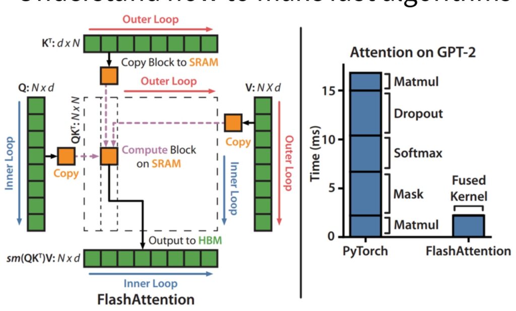
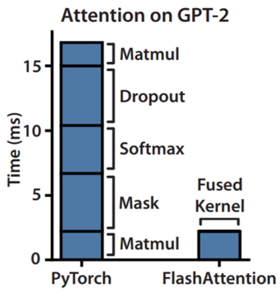
Let’s dive into Flash Attention, which beautifully demonstrates how all the GPU optimization tricks we’ve learned come together in practice. I’m going to try to make it so that all the tricks that I taught you aren’t these random disconnected facts about GPUs. They’re kind of part of the standard performance optimization toolkit, and Flash Attention and Flash Attention 2 will hopefully teach you how that all comes together to build one of the foundations of modern high performance transformers. Flash Attention dramatically accelerates attention computation, and most of you probably know that’s done through some CUDA kernel magic. What the paper shows is that if you take attention on an unoptimized PyTorch transformer implementation and fuse the kernel while doing some optimizations, you can get significant, significant speed ups.
The Flash Attention Strategy
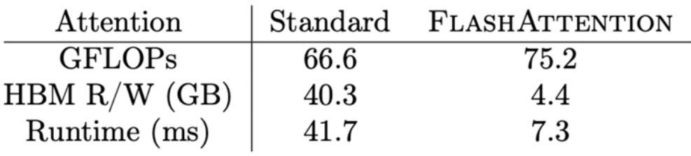
From the paper, they say we apply two established techniques – tiling and recomputation – to overcome the technical challenge of computing exact attention and subcredits quadratic HBM accesses. It’s not subcredits computation, because you can’t do that – you have to compute attention in general. But they’re going to get subcredits accesses to the high bandwidth memory or global memory, and that’s really the key.
Memory is the bottleneck. You want to make that not quadratic, so that at least you can pay for a quadratic cost with your compute rather than with your memory.
Now that we’ve seen the impressive performance gains Flash Attention achieves, let’s step back and understand exactly what makes attention computation so challenging from a mathematical perspective. To properly appreciate the elegance of Flash Attention’s solution, we need to review the core attention mechanism and identify where the computational bottlenecks really lie.
Attention Mechanism Mathematical Review
The attention mechanism fundamentally relies on three different matrix multiplications involving the key (\(K\)), query (\(Q\)), and value (\(V\)) matrices, with a crucial softmax operation positioned between them. These matrix multiplications themselves are relatively straightforward computationally and can be efficiently handled using standard tiling techniques that we’ve discussed for optimizing matrix operations.
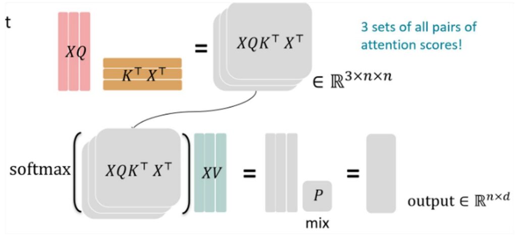
🔴 The Softmax Challenge
However, what makes attention computation particularly challenging is the softmax operation that sits right in the middle of this process. This softmax step is going to be the real tricky bit that we need to tackle carefully. The softmax introduces numerical stability concerns and requires special handling to ensure we don’t run into overflow or underflow issues during computation.
💡 The Key Insight
Once we can effectively deal with the softmax computation and its associated challenges, all of the matrix multiplication optimization techniques and tiling strategies that we’ve been discussing will naturally come into play. The key is solving that softmax bottleneck, and then the rest of the attention mechanism can leverage the same efficient computational patterns we use for standard matrix operations.
This understanding sets the stage for appreciating how Flash Attention’s clever algorithmic innovations address these exact challenges.
14. Flash Attention Tiling Implementation
Matrix Multiplication Tiling for Attention
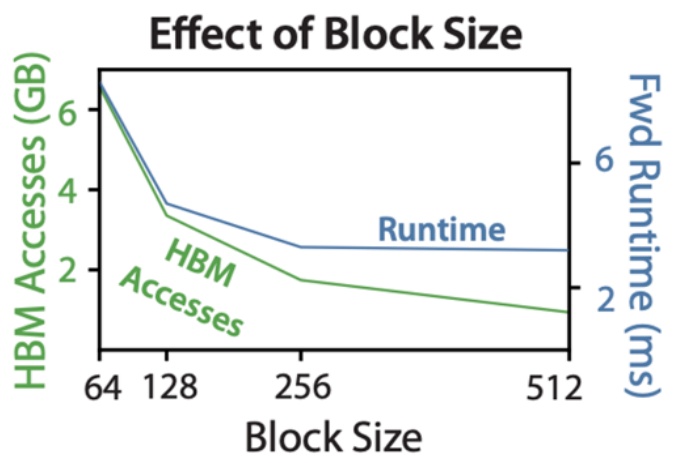
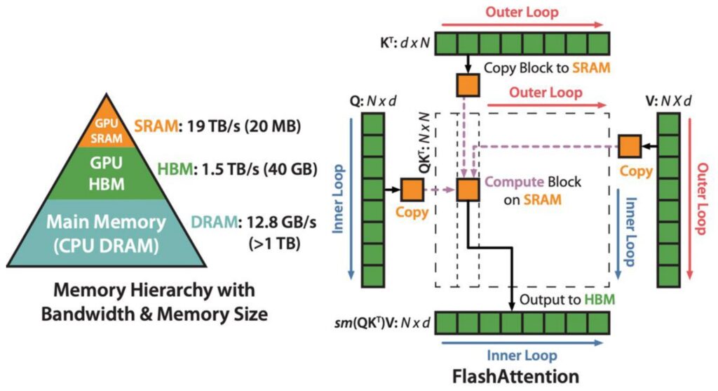
Let’s dive into the FlashAttention approach, which is essentially a clever implementation of tiled matrix multiplication for the attention mechanism. The core concept is beautifully simple: we take the \(K\) matrix and \(Q\) matrix and divide them into small, manageable blocks. These blocks are then copied into SRAM where the actual multiplication takes place, followed by accumulation before being sent to HBM for softmax operations and subsequent multiplication with \(V\).
🔴 The Softmax Problem
However, the real challenge emerges when we consider the softmax operation. The fundamental problem with softmax in attention is that it’s inherently a global operation that must process entire rows. To compute the normalizing term, you need to sum across the complete row, which creates a significant computational bottleneck when working with tiled approaches.
The ideal scenario for efficient tiled computation would be to perform all operations within individual tiles without ever needing to write back to the larger matrix. This requires developing a softmax that can be computed online within each tile, maximizing the amount of computation we can accomplish locally. This brings us to the crucial innovation that makes FlashAttention possible.
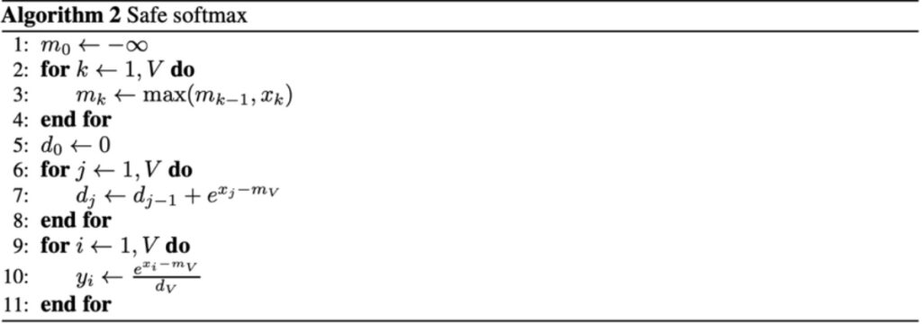
Incremental Softmax Computation
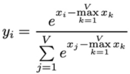
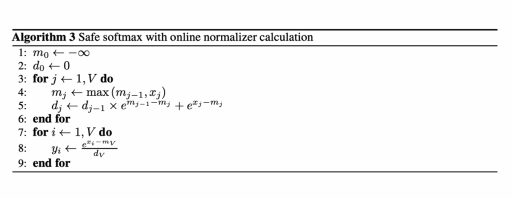
The key innovation that solves our tiling challenge is using what’s called the online softmax algorithm. In the traditional batch version of softmax, you take all of your values \(x_1\) through \(x_n\), exponentiate them, sum them, and divide. You also compute the maximum value and subtract it to ensure numerical stability. The online softmax, developed by Nikolau and Gimelstein in 2018, allows you to compute this incrementally by maintaining a current running normalizer term and the current top term of \(e^{x_i – \max x_k}\).
How Online Softmax Works
The algorithm maintains your current max that you’ve seen over \(x_1\) through \(x_j\) (where \(j\) is your current iteration), along with a correction term that updates when the max changes. The variable \(d_j\) tracks the top term of the equation online, and at the end, you can compute the normalizer to get the normalized \(y_i\) that you want.
The crucial advantage is that this can be done online – you don’t need \(x_1\) through \(x_n\) up front, just a stream of values. This enables computing the softmax tile by tile, where within each tile you run this algorithm to compute the partial softmax for that tile.
This approach means you never have to materialize the full \(n^2\) matrix to compute the softmax. In the FlashAttention implementation, you start with your \(K\) and \(Q\) matrix multiply using tiled chunks. You maintain a running value of the exponentiated sums and incrementally update while correcting for the maximum terms. By computing all necessary quantities tile by tile, you can then multiply with tiles of \(V\) at the end to get your full softmax output. While you do need to go through all tiles before outputting the final softmax (since you need the complete denominator sum), once you’ve processed all \(n^2\) tiles, you have all components needed to directly output the softmax without recomputation.
💡 Backward Pass Strategy
For the backward pass, the same principle applies – you perform recomputation tile by tile to avoid storing anything of size \(n^2\). Since storing the activations would already require \(n^2\) memory, you instead recompute them on the fly tile by tile during the backward pass. This recomputation strategy is a key trick that makes the backward pass memory-efficient. Now let’s see how all these pieces come together in the complete implementation.
Complete Flash Attention Forward Pass
Now that we understand both the tiling strategy and incremental softmax computation, let’s put it all together in the complete forward pass of flash attention. The process begins with your \(KQ\) matrix multiply using tiled chunks that are multiplied together. To compute the softmax efficiently, you maintain a running value of the exponentiated sums and keep incrementally updating it while correcting for the maximum terms. This tile-wise computation of the inner products (\(S\)) includes fusion of the exponential operator, allowing you to compute all necessary quantities tile by tile as you progress from one tile to another.
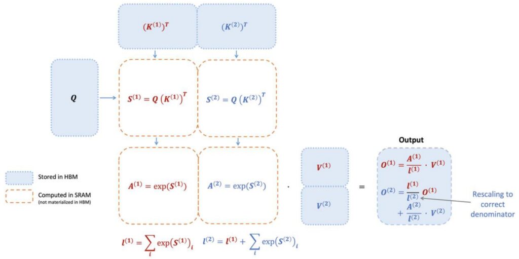
Single Pass Efficiency
The key insight is that while you need to process all tiles before you can output the final softmax, you only need to go through all the \(n^2\) tiles once. After completing this single pass through all tiles, you have all the components necessary to directly output the softmax without requiring recomputation. This is because you’ve already built up the normalizer terms – specifically \(L\) (the sum of all exponentiated terms) – which remains in shared memory after processing the last tile. With these components available, you can perform the final exponentiation and division to return all the required outputs.
The backward pass, while not covered in detail here, employs a crucial memory optimization strategy. Since storing activations would require \(n^2\) memory (which we want to avoid), the algorithm performs recomputation tile by tile during the backward pass. This approach prevents storing any \(n^2\) components during the forward pass computation, and similarly avoids storing \(n^2\) activations during backpropagation. Instead, activations are recomputed on the fly tile by tile when needed for gradient computation. This recomputation strategy is a key trick that makes the memory-efficient backward pass possible, while the actual gradient computation follows standard procedures, just executed tile by tile. This completes our understanding of how FlashAttention achieves its remarkable memory efficiency while maintaining computational accuracy.
15. Course Summary
Hardware Optimization Recap
As we wrap up our deep dive into hardware optimization, I hope you’ve seen how all the pieces I talked about regarding tiling, coalescing, and re-computation come together to give you flash attention and all these really cool optimizations that make your transformers go much faster. To recap for the whole lecture, hardware is fundamentally the thing that has powered all of the language models we have today. If you really want to leverage your hardware effectively, you have to understand and engage with the low-level details—all the major systems advances really build upon the concepts I’ve taught today.
🔴 The Critical Insight: Memory Movement
The current GPU scaling plot is really the one you should remember—it really incentivizes and encourages you to think about memory movement. Memory movement is the bottleneck in all of this. You don’t want to just think about reducing the number of FLOPS, though that’s important too. You really have to think about how to make your memory movements more efficient.
Summary – The Path to Optimal Performance
Finally, if you have to do a certain amount of computation, the way to optimize things is to optimize your data movement to avoid as much movement from high bandwidth memory or global memory as possible. You want to reduce that and have everything in the very, very fast shared memory. This approach leads to good performance on algorithms like flash attention and represents the key insight for modern hardware optimization that will serve you well as you build and deploy your own models.
This post is written based on Large Language Models From Scratch Lecture 5. Stanford University.