LLMs Scratch #004: Mixture of Experts (MoE) Models: The Architecture Powering 2025’s Best AI Systems
🎯 What You’ll Learn
This comprehensive guide takes you from MoE fundamentals to state-of-the-art implementations like DeepSeek V3. You’ll understand why sparse architectures outperform dense models at every compute scale, master the critical routing mechanisms that determine expert selection, and learn the training techniques that make these complex systems work. We’ll examine real benchmark results from Llama 4, Grok, and DeepSeek, explore load balancing challenges and solutions, and walk through the complete evolution of DeepSeek’s architecture from V1 to V3. Whether you’re building production systems or understanding frontier AI, this is the essential knowledge you need.
Complete Tutorial Overview
Part 1: Introduction to Mixture of Experts
- MoE Fundamentals and Motivation — What MoE models are, dense vs sparse architectures, computational efficiency
- MoE Performance Results — Western and Chinese model benchmarks, historical adoption challenges
Part 2: MoE Architecture and Routing Mechanisms
- Core MoE Architecture — General structure, MLP vs attention routing, design questions
- Routing Functions and Methods — Token choice, expert choice, top-\(k\) implementation details
- Recent Routing Innovations — DeepSeek fine-grained experts, shared experts, configuration studies
Part 3: MoE Training Methods and Challenges
- Training Approaches — Non-differentiable routing, RL methods, stochastic approximations
- Load Balancing and Expert Allocation — Heuristic losses, DeepSeek balancing, auxiliary loss-free training
- Training Challenges and Solutions — Expert parallelism, stochasticity issues, stability and overfitting
Part 4: Advanced MoE Techniques and Case Studies
- Model Upcycling Techniques — Dense to MoE conversion, MiniCPM and Qwen examples
- DeepSeek MoE Evolution — V1 to V3 architecture progression, sigmoid gating
- Complete MoE Implementation — Multi-Head Latent Attention, Multi-Token Prediction, summary
Part 1: Introduction to Mixture of Experts
Understanding the fundamentals and real-world performance
1. MoE Fundamentals and Motivation
What Are Mixture of Experts Models
Let’s start by understanding what Mixture of Experts (MoE) models actually are and why they’ve become absolutely critical in 2025 thanks to widespread adoption across the industry. This year has brought tremendous developments in MoE architectures, and we’ll explore everything from the fundamentals to cutting-edge systems like DeepSeek V3 to understand what makes state-of-the-art open-source architectures tick.
The MoE Landscape in 2025
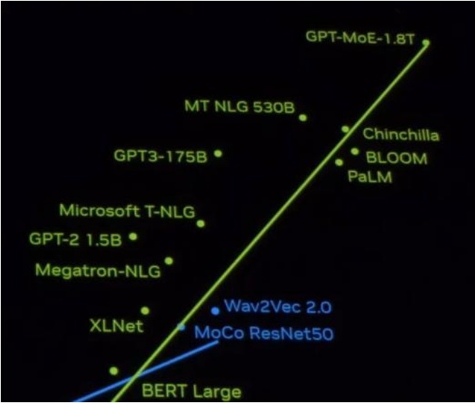
The landscape has shifted dramatically. There was that amusing leaked video suggesting GPT-4 might actually be “GPT-MoE-1BT,” and now major players like Grok, DeepSeek, and Llama 4 have all embraced mixture of experts architectures. At this point, the advantages of MoE over dense architectures are crystal clear: at almost any compute scale, training a well-implemented mixture of experts model will outperform a dense model.
Key insight: This makes MoE essential knowledge for anyone trying to build the best possible model within their computational budget.
🔴 Common Misconception About “Experts”
Despite its name, Mixture of Experts is quite different from what you might initially imagine. You’d naturally think there are specialized experts for different domains—like a coding expert, an English expert, or experts for other languages—but that mental model is completely wrong.
MoE is actually a sophisticated architecture featuring multiple sub-components called “experts” that are activated sparsely during computation. The real action happens in the MLPs (Multi-Layer Perceptrons).
💡 The Key Architectural Insight
Here’s the key insight: MoE and non-MoE architectures are nearly identical in all components except one crucial difference.
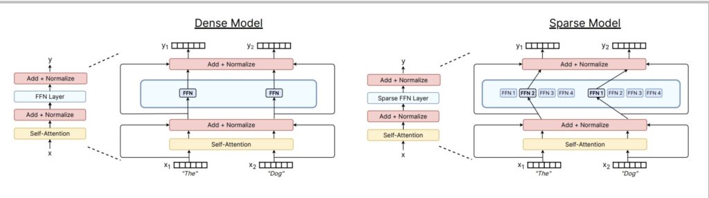
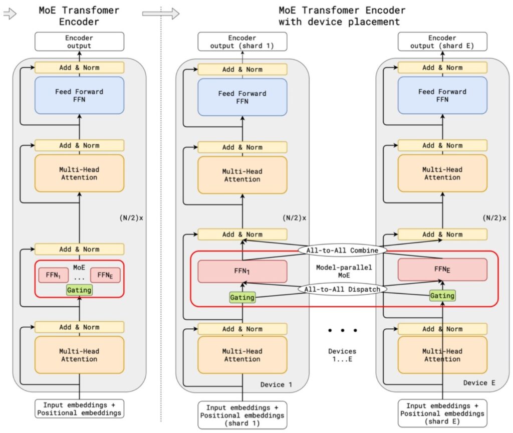
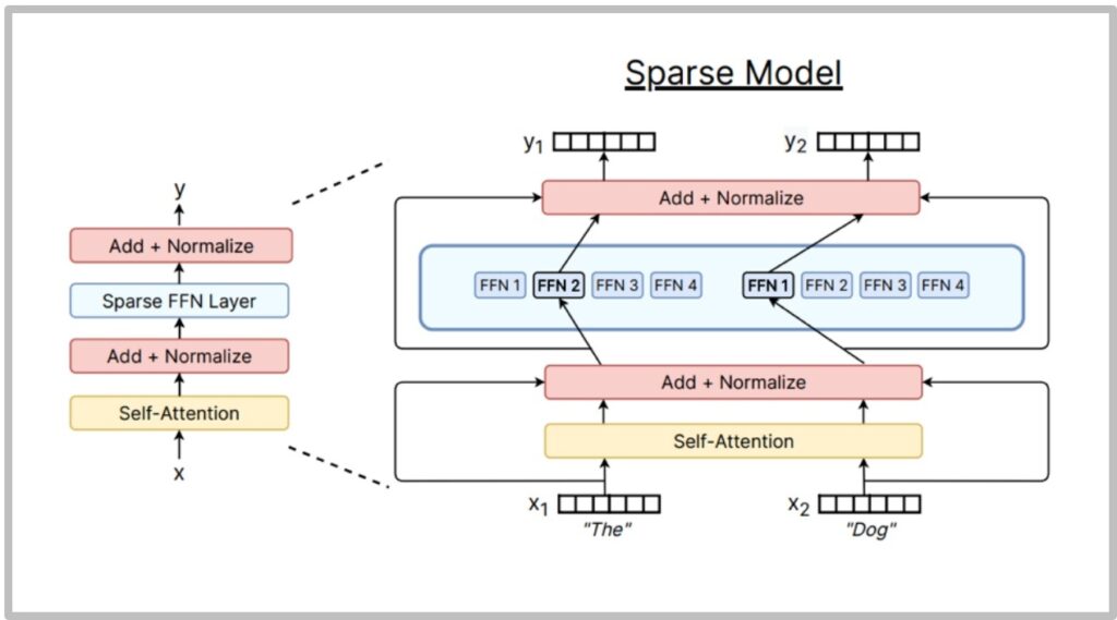
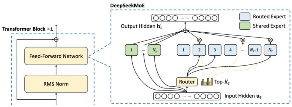
Looking at a standard transformer’s components—self-attention and feed-forward networks (FFNs)—the magic happens when we transform that single large FFN block. In a dense model, you have one big feed-forward component doing all the work. In a sparse MoE model, we split or copy this FFN into multiple smaller networks, then add a router that selectively activates only some of these experts during each forward pass.
The Beauty of Computational Efficiency
The beauty of this approach lies in its computational efficiency. If the system sparsely activates experts—say, picking just one expert per forward pass, where each expert matches the size of the original dense FFN—then the FLOP count remains identical between dense and MoE models.
You’re performing the same matrix multiplications during inference, but now you have significantly more parameters without increasing computational cost. If you believe that model performance benefits from having more parameters to memorize facts about the world, this architecture is incredibly compelling.
Reasons for MoE Popularity Growth
The theoretical advantages I just described are backed by compelling empirical evidence.
Empirical Evidence: More Experts = Better Performance
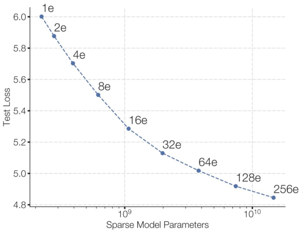
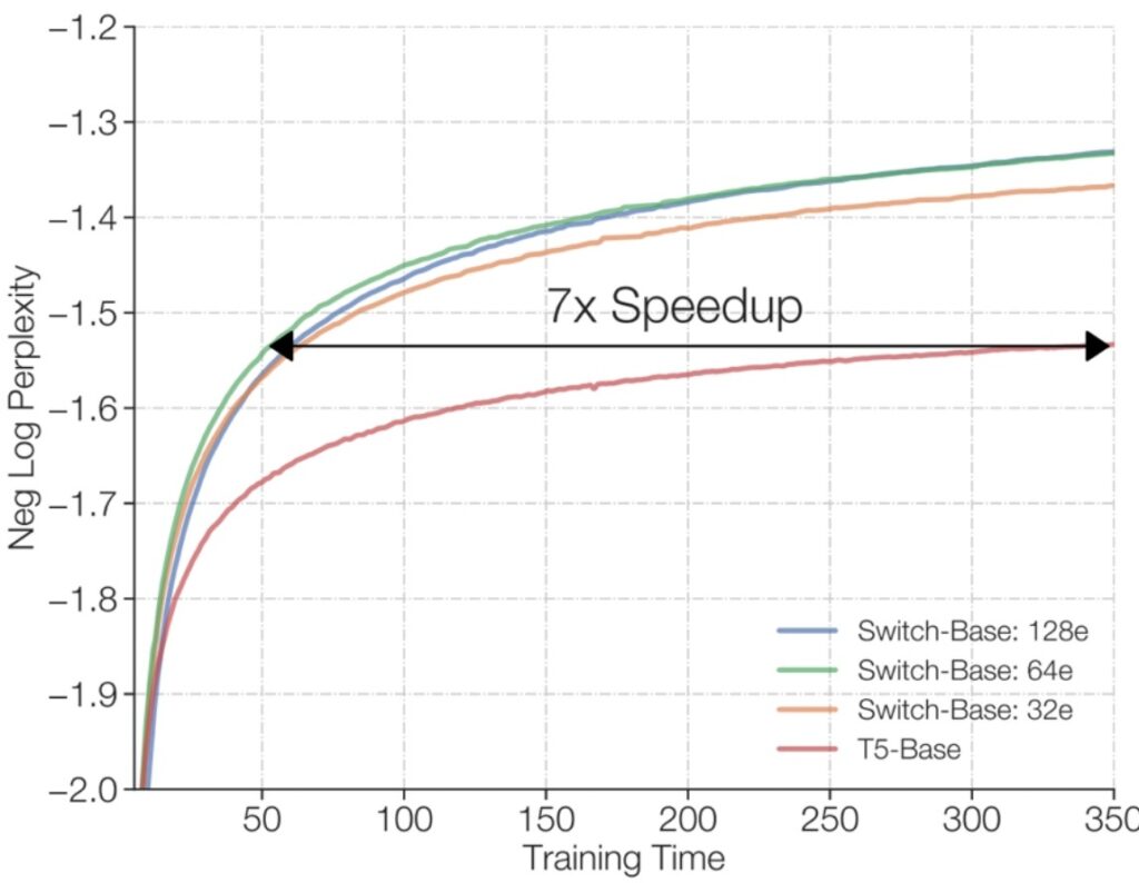
One of the most convincing demonstrations of MoE effectiveness comes from Fedus et al. (2022), where they show that if you match your training flops—using the same amount of compute for training—the training loss of your language model keeps decreasing as you increase the number of experts. More experts simply perform better.
💡 The Trade-off to Consider
Of course, experts aren’t free—you need to store memory for these experts, and when you implement parallelism, you have to handle routing data into 256 separate experts, creating systems complexities. But if you’re only thinking about flops, this creates a great situation where you have the same computational cost but get significantly better test loss.
Modern Validation: AI2’s Olmo Paper
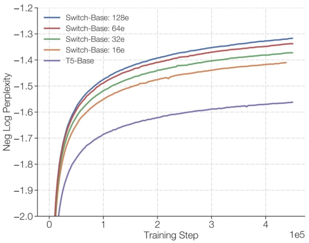
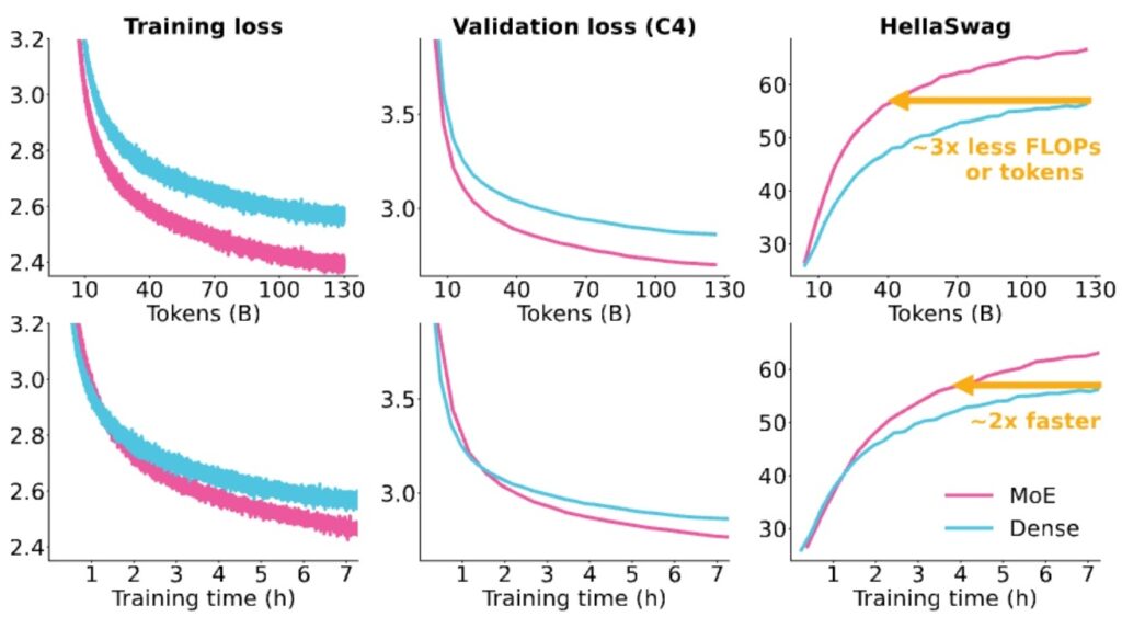
You might wonder if this 2022 result holds true for modern architectures at modern scales—and it absolutely does. AI2’s excellent Olmo paper conducted careful ablations and controlled comparisons between dense versus MoE architectures, seeing exactly the same patterns.
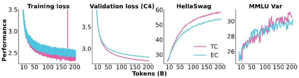
The results show a \(7\times\) speedup from having many experts, and in the Olmo comparison, the MoE model (shown in pink) significantly outperforms the dense T5-Base model, with training loss decreasing much more rapidly for MoE than for dense architectures.
🔴 The Systems Complexity Price
While we pay a price in systems complexity, at the flops level this looks very compelling. One drawback is the significant systems complexity required to make MoE efficient—which is why it’s not the standard architecture taught in introductory courses. However, when implemented properly, especially with each expert living on a separate device for efficient data routing, you can put all your flops to productive use.
Expert Parallelism: A New Axis of Scaling
Another major systems benefit is that MoEs provide an additional axis of parallelism called expert parallelism. When you need to distribute your model across many devices, experts offer a natural cutting point—you can place each expert on a different device and simply route tokens to the appropriate device for computation.
This has made MoEs particularly popular for scaling really large models. Interestingly, while MoEs were developed at Google and adopted by many frontier labs, much of the open research initially came from Chinese groups like Qwen and DeepSeek. Only recently have Western open source groups and companies like Meta (with Llama’s MoE architecture) begun extensive MoE work.
2. MoE Performance Results
Western Model MoE Results
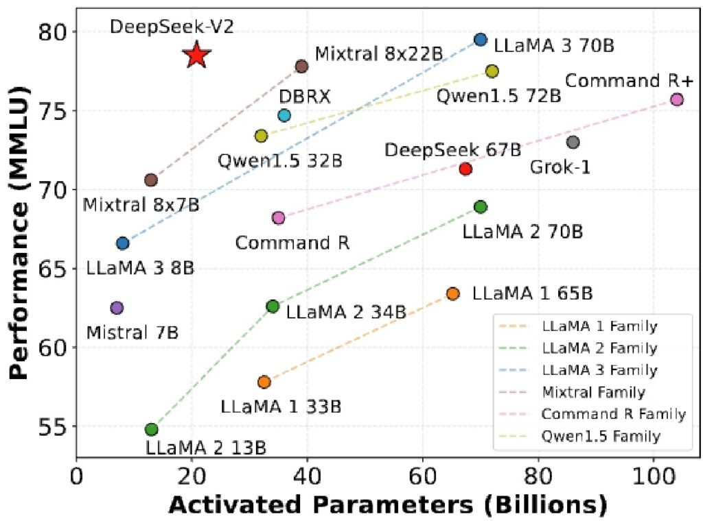
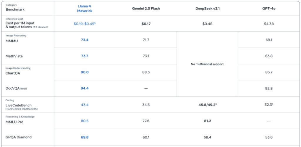
Let’s examine how Mixture of Experts architectures have transformed the landscape of high-performance AI models. With the latest release of Llama 4, we’re seeing continued innovation in sparse MoE designs that deliver exceptional performance while maintaining computational efficiency.
The Current State of MoE Models
What’s particularly noteworthy is that MoEs now represent most of the highest-performance open models available today, and they’re remarkably quick in their inference capabilities. Much of the foundational work in this area has come from Chinese research groups, particularly Qwen and DeepSeek, who have conducted extensive benchmarking and evaluation studies.
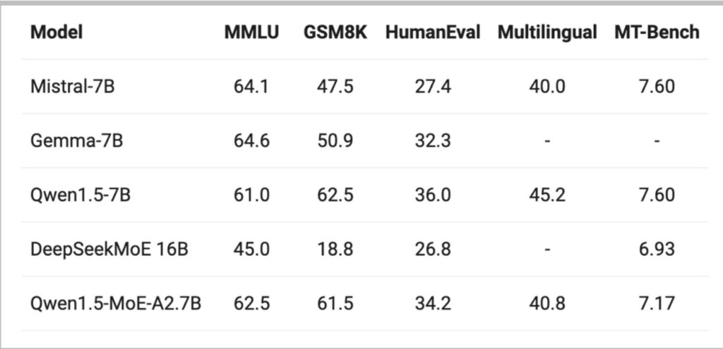
💡 Qwen’s Upcycling Innovation
Qwen 1.5 stands out as one of the first models to demonstrate large-scale, well-tested, and thoroughly documented MoE implementation. Their approach was particularly innovative—they developed a clever technique to upcycle an existing Qwen 1.5 dense model into a mixture of experts architecture.
This upcycling approach represents a significant breakthrough in model development efficiency, allowing researchers to leverage existing dense model weights and transform them into more capable sparse architectures.
Chinese Model MoE Results
Building on the foundational work we just discussed, one of the most clever architectural innovations in recent years has been the technique of taking a dense model and transforming it into a Mixture of Experts (MoE).
Dense to Sparse: A Paradigm Shift
This approach demonstrates significant gains in compute efficiency while actually decreasing the total number of parameters relative to traditional dense models. This represents a fundamental shift in how we think about model scaling and efficiency.
🔴 DeepSeek’s Foundational Contributions
DeepSeek, which has now become famous but wasn’t quite as well-known when these foundational papers were first emerging, conducted some of the most important MoE work in the open source world. A significant portion of understanding modern MoE architectures involves tracing the trajectory of DeepSeek’s innovations.
Their original DeepSeek MoE paper presents beautifully controlled comparisons examining what happens when you train a dense model with a particular amount of FLOPs, versus training a naive MoE without smart routing, versus using more sophisticated routing like the Switch MoE approach.
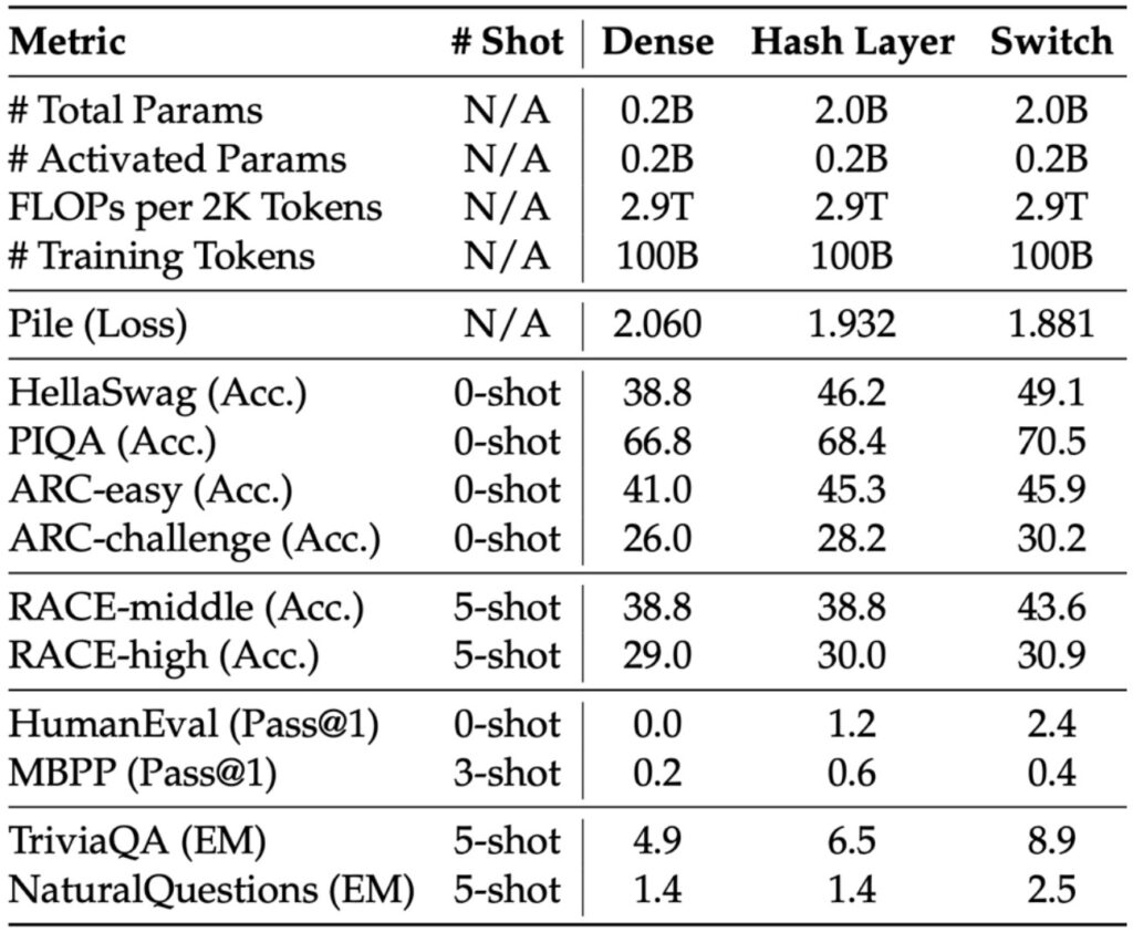
Consistent Pattern: Sparse Outperforms Dense
The results from these carefully controlled experiments reveal a consistent pattern: as you progress from dense to sparse architectures—moving from the leftmost to rightmost columns in their comparisons—you see benchmark metrics consistently improving for a fixed amount of computational budget.
Recent ablation work on MoEs has further reinforced that these architectures are generally beneficial across a wide range of applications and use cases.
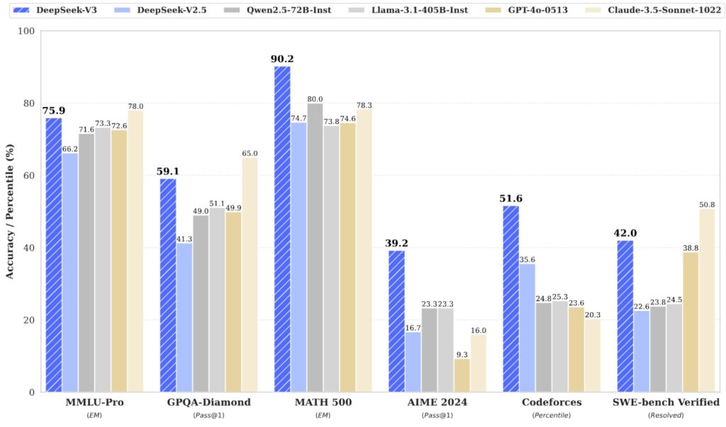
💡 DeepSeek V3: Engineering Excellence
While most people have probably heard of DeepSeek V3 by now, which represents the culmination of this entire line of research, those who had been following MoE developments would have known about DeepSeek long before V3 gained widespread popularity.
What’s particularly fascinating is that DeepSeek V3 is architecturally not very different from the earliest DeepSeek MoE models—they had essentially solved the core architectural challenges when they were still working with much smaller 2 billion parameter models. The real breakthrough with V3 was getting the engineering implementation right to create something that is genuinely remarkably good.
Historical Adoption Challenges
Given all these impressive results, there’s a natural question: why haven’t MoEs been more popular? Why isn’t it the standard thing we teach in NLP and language modeling classes?
🔴 The Complexity Problem
It’s just that they’re very complex and they’re very messy. The infrastructure is very complex, and the biggest advantages of MoEs really happen when you’re doing multi-node training—when you have to split up your models anyway, then it starts to make sense to shard experts across different devices. But until you get to that point, maybe MoEs are not quite as good.
Some of the earlier Google papers really talk about this trade-off where they say, actually, when you get these really big models that you have to split up, then experts become uniquely good.
The Non-Differentiability Challenge
If you think about it carefully, this decision of which expert you route tokens to is a very difficult thing to learn. In deep learning, we really like differentiable objectives—very smooth things that we can take gradients of.
Routing decisions are not differentiable, because we have to pick and commit to a particular expert. So if we’re doing that, we’re going to have a very tricky optimization problem. And the training objectives to make that work are either heuristic and/or unstable.
Part 1 Key Takeaways
- MoE = Sparse FFN activation: Replace one large FFN with multiple smaller experts + router
- Same FLOPs, more parameters: Computational cost stays constant while capacity increases
- \(7\times\) training speedup: Empirically validated across multiple studies (Fedus 2022, Olmo)
- Expert parallelism: Natural distribution of experts across devices for large-scale training
- Chinese leadership: DeepSeek and Qwen pioneered much of the open MoE research
- Adoption barriers: Systems complexity and non-differentiable routing remain challenges
Part 2: MoE Architecture and Routing Mechanisms
Understanding the core structure and how tokens find their experts
3. Core MoE Architecture
General MoE Structure and Variations
Now let’s dive into the core architecture of MoE models. What do Mixture of Experts (MoE) models actually look like? The classic MoEs that you should think of are where you take the densely connected layers—the feed-forward networks (FFNs)—and you split them up or copy them, creating sparse routing decisions among them. The fundamental idea is to replace the traditional MLP components with multiple expert networks that can be selectively activated based on the input.
The Classic MoE Pattern
The standard approach is straightforward: you have a router of some kind, and you route to different MLPs or expert networks. This raises several critical design questions that we need to address throughout this section.
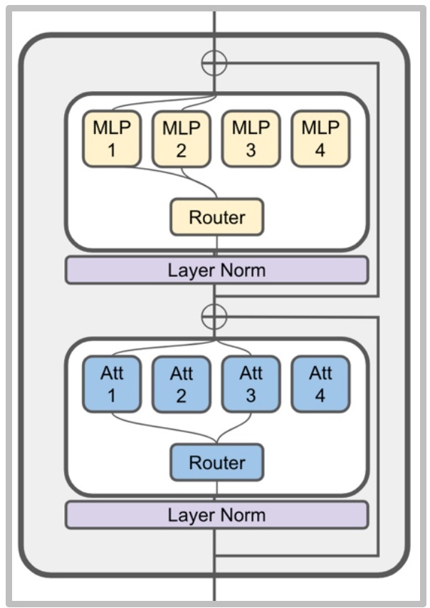
💡 What About MoE Attention?
You could also have a sparsely routed attention layer, and there have been a couple of papers and releases that have taken this approach. However, it’s actually quite rare to see this in major model releases.
This approach is reportedly much more unstable and very difficult to train consistently. There haven’t been many ablations to confirm this, but certainly, there haven’t been many people training those kinds of models with MoE attentions.
Critical Design Questions
The standard approach raises several critical design questions that we need to address:
- How do we route? The routing function is obviously an important choice that determines which experts get activated for which inputs.
- How many experts should we have, and how big should each expert be? These are fundamental architectural decisions that affect both model capacity and computational efficiency.
- How do we train this router? This involves dealing with what appears to be a non-differentiable objective that seems very difficult to train effectively.
🔴 The Training Challenge
The final and perhaps most challenging question is: how do we train this router? This involves dealing with what appears to be a non-differentiable objective. These are very important design questions, and we’re going to go through each one in detail, hopefully covering the design space of all these MoE approaches.
If you’re interested in understanding a broad overview of MoEs, at least circa 2022, there’s a really nice survey or review paper by Fedus et al. from 2022 that covers a lot of these fundamental concepts and variations.
4. Routing Functions and Methods
Routing Function Overview and Types
Now that we understand the basic architecture of Mixture of Experts models, let’s dive into their most critical component: the routing function. When sequences come into the system, these tokens need to be assigned to specific experts, but crucially, not all experts will process every token. This sparse routing is the fundamental advantage of MoEs.
Three Primary Routing Strategies
There are three primary routing strategies we can employ:
- Token Choice: Each token develops a preference ranking for different experts, and we select the top \(k\) experts for each token.
- Expert Choice: Works in reverse—each expert ranks tokens by preference and selects the top \(k\) tokens to process, which provides excellent load balancing across experts.
- Global Assignment: Involves solving a complex optimization problem to ensure balanced mapping between experts and tokens.
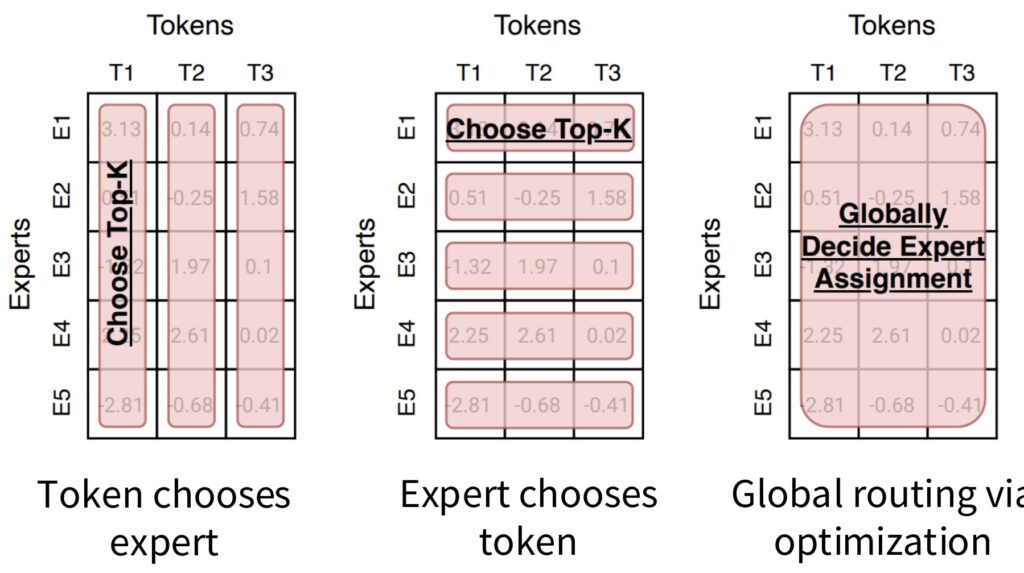
Token Choice Dominates Modern MoEs
Despite the theoretical appeal of different routing mechanisms, almost all modern MoEs have converged on token choice top-\(k\) routing. In the early days, researchers explored the entire spectrum of routing possibilities, but major releases consistently adopt this single approach.
💡 How the Router Works
The routing mechanism itself is surprisingly lightweight. When a token represented by vector \(\mathbf{x}\) enters the system through the hidden residual stream, the router simply multiplies \(\mathbf{x}\) by a weight matrix \(W\) and applies an activation function like sigmoid to generate scores.
This creates a vector-vector inner product operation, similar to attention mechanisms. The routing function depends on both the token’s position and its hidden state after processing with position embeddings.
The Choice of \(k\)
The choice of \(k\) represents a crucial hyperparameter with interesting trade-offs. While \(k=1\) might seem optimal for efficiency, early MoE papers argued that \(k \geq 2\) provides valuable exploration benefits—if we always exploit the best expert, we miss opportunities to discover potentially better alternatives.
Key insight: The second-best expert in \(k=2\) routing offers exploration information that can improve overall performance. However, increasing \(k\) directly multiplies computational cost: \(k=2\) doubles the FLOPs compared to \(k=1\).
Top-K Routing Methods
Building on our understanding of routing fundamentals, let’s dive deeper into top-\(K\) routing methods in mixture of experts (MoE). The earliest MoE papers argued that when \(K > 2\), you get valuable exploration benefits.
🔴 Why \(K = 2\) Became Standard
If you’re doing \(K = 1\), you might always be exploiting the best expert and never discover other potentially useful options. But when \(K = 2\), that second expert can provide exploration information. This is why \(K = 2\) became the canonical choice and remains very popular today, though it does double the computational cost (FLOPs).
Top-\(K\) Routing in Practice
Top-\(K\) routing is the dominant approach used in most MoE implementations:
- Switch Transformer: \(K=1\)
- GShard, Grok, Mixtral: \(K=2\)
- Qwen, DBRX: \(K=4\)
- DeepSeek: \(K=7\)
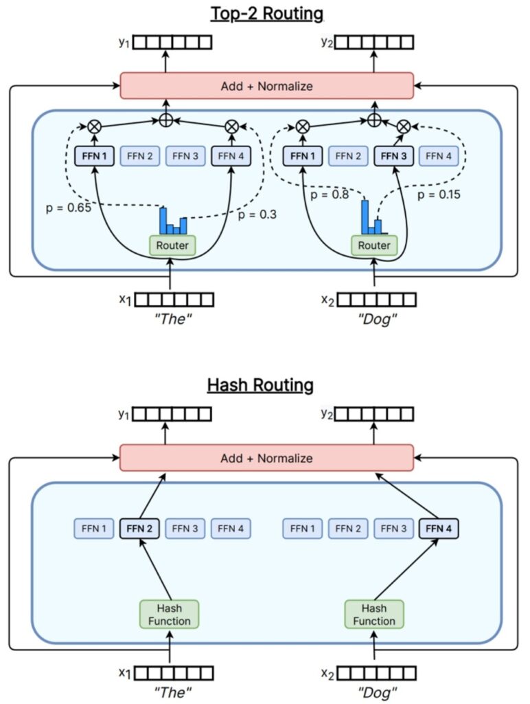
The mechanism works by taking residual stream inputs \(X\) and feeding them into a router—essentially an attention-like operation with a linear inner product followed by softmax. The router selects the top-\(K\) most highly activated experts, and their outputs are then gated and combined.
💡 Surprising Finding: Hash Routing Works Too
Interestingly, research has shown that you don’t even need sophisticated routing at all. You can use simple hashing functions to map inputs \(X\) onto experts, and even without any semantic information, hashing-based MoEs still provide significant gains—which is quite remarkable.
This suggests that much of the benefit comes from the increased model capacity rather than intelligent routing decisions.
Alternative Approaches (Largely Abandoned)
While top-\(K\) routing dominates current practice, researchers have explored more sophisticated approaches:
- Reinforcement Learning: Some early MoE work used RL to learn routing behavior, recognizing that routing choices are discrete decisions well-suited to RL optimization. However, this approach has largely been abandoned due to prohibitive computational costs and stability issues.
- Linear Assignment / Optimal Transport: Elegant approaches using linear assignment problems have been proposed, but their computational overhead outweighs their practical benefits.
Detailed Top-K Implementation
Let’s now examine the specific top-\(k\) routing implementation that almost everyone has converged to. This is the router that’s used in DeepSeek V1 to V2, and models like Qwen and Grok do almost exactly this.
The Standard Top-\(K\) Router Equations
The process begins with inputs \(\mathbf{u}^l\) from the residual stream. To process this through our MoE, we first determine which experts are going to be activated:
$$\mathbf{h}_t^l = \sum_{i=1}^N \left( g_{i,t} \text{FFN}_i \left( \mathbf{u}_t^l \right) \right) + \mathbf{u}_t^l$$
$$g_{i,t} = \begin{cases} s_{i,t}, & s_{i,t} \in \text{Topk}(\{s_{j,t} | 1 \leq j \leq N\}, K), \\ 0, & \text{otherwise}, \end{cases}$$
$$s_{i,t} = \text{Softmax}_i \left( \mathbf{u}_t^{lT} \mathbf{e}_i^l \right)$$
Understanding the Equations
How we determine expert activation is very similar to attention. We take our \(\mathbf{u}\), which is our residual stream input, and compute inner products with the \(\mathbf{e}_i\)’s (expert embeddings).
This becomes like a weighted selection operation over \(K\) different (or actually \(N\) different) FFNs. The \(\mathbf{u}^l\) at the very end is the residual stream—we’re adding back the inputs because we want an identity connection through it.
🔴 Why Is the Router So Simple?
A natural question arises: why does the router have such a basic parameterization? What happens if you put more weights in your router?
The complex answer is that systems concerns weigh heavily. If you’re using a lot of FLOPs to make routing decisions, you have to pay for those FLOPs, and you need to get performance improvements that justify the routing overhead.
There are also really big limits to how well you can route because the learning process for routing is actually pretty dicey. The only thing you have is if you use top-two, then you can compare the two things that you have—but that’s a very indirect way to be learning your affinity.
💡 DeepSeek’s Innovation: Shared + Fine-Grained Experts
One of the great innovations of the DeepSeek MoE, which was very quickly adopted by other Chinese MoE releases, is the idea of both a shared expert and fine-grained experts.
This architectural innovation addresses the routing limitations while maintaining computational efficiency—a topic we’ll explore in depth in the next section.
Part 2 Key Takeaways
- MoE = Replace FFN with routed experts: Standard approach applies MoE to MLPs, not attention
- Three routing strategies: Token choice (dominant), expert choice, global assignment
- Top-\(K\) is universal: \(K=2\) most common, balancing exploration vs computation
- Router is simple by design: Complex routers don’t justify their FLOP overhead
- Hash routing works: Benefits come from capacity, not just intelligent routing
- DeepSeek innovations: Shared + fine-grained experts address routing limitations
5. Recent Routing Innovations
DeepSeek and Chinese Model Variations
Now let’s explore some of the most impactful recent innovations in routing architectures. The basic mixture-of-experts (MoE) structure that was originally proposed takes your dense architecture and essentially copies the experts over.
The Vanilla MoE Starting Point
In this case, if you have top-\(k\) routing with \(k=2\), you’re going to have twice the activated parameters as your original dense model. So you take your MoE and copy it over and activate \(k=2\). This is what you might think of as the vanilla or basic MoE that you might start with.
Key insight: People realized fairly quickly that having lots of experts is good, and the logical next step beyond having lots of experts is wanting lots of experts without paying the parameter cost for having lots of experts.
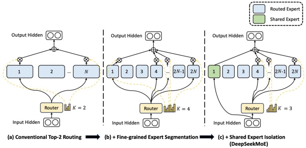
DeepSeek’s Fine-Grained Expert Innovation
DeepSeek basically argued that the right thing to do was to cut the expert up into smaller pieces. Remember the golden rule is to have your hidden layer and then multiply that by four to give you your projection layer. Now what you would do is instead of multiplying by four, you might multiply by two. So now you have smaller matrices, more fine-grained experts, and you can have twice as many of them.
💡 Scaling Fine-Grained Experts
You can take that logic much more to the extreme—you can quadruple or multiply by eight, and keep decreasing the size of your projection dimension there. That’s fine-grained experts, though it doesn’t come for free, so you have to be very careful about how you structure these things.
Shared Experts for Common Processing
The other innovation that has been studied is having at least some MLP that can capture shared structure. Maybe there’s processing that always needs to happen no matter which token you’re processing.
In that case, it seems like a waste to do all this routing work and have parameters spread out everywhere when we can just have one shared or a few shared experts whose job it is to handle all of this shared processing that’s needed.
🔴 The Ablation Evidence
This setup of using fine-grained experts plus shared experts originally came out in DeepSeek MoE, though the original inspiration came from DeepSpeed MoE. Almost all of the open MoE releases since DeepSeek have adopted some sets of these innovations, because it’s quite clear that especially fine-grained experts is just really, really useful—that’s a no-brainer at this point.
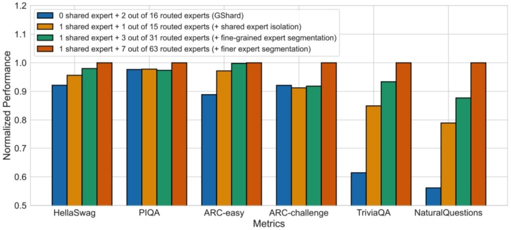
The ablation in the DeepSeek MoE paper shows:
- Blue bar (G-shard): Very basic vanilla implementation
- Orange bar (one shared expert): Big boost on some tasks
- Green bar (fine-grained experts): Further boosts
- Composing all differences: Quite the big boost overall
Expert Configuration Studies
Independent research has provided valuable validation and refinement of these DeepSeek innovations.
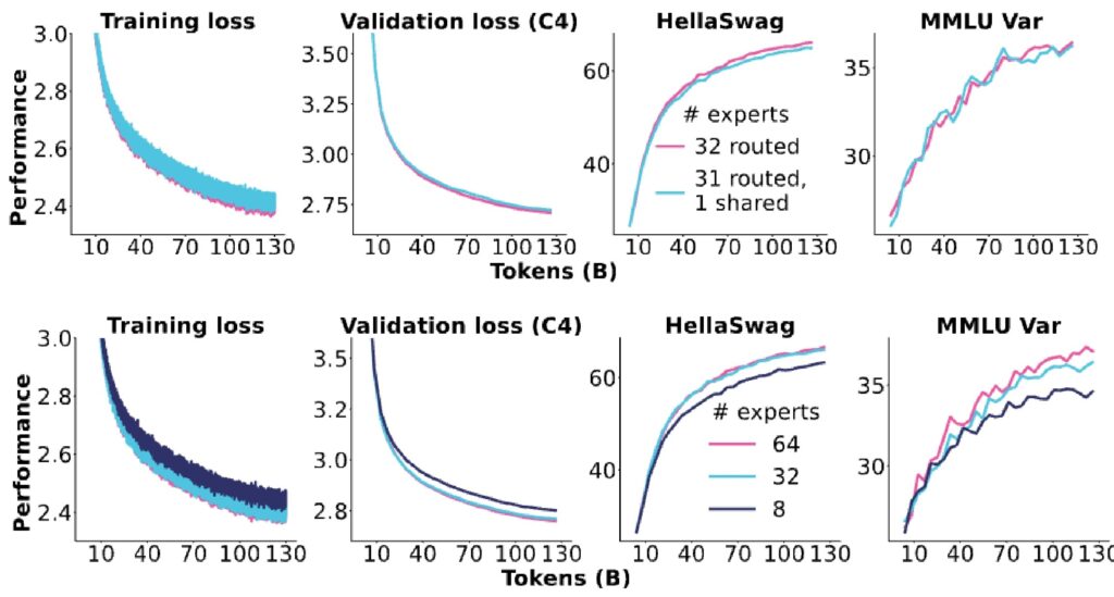
Independent Validation Results
Looking at the experimental results, we see very clear trends in losses and other metrics showing improvements going from 8 to 32 to 64 experts. Fine-grained experts demonstrate significant gains, while shared experts (shown in purple versus teal) don’t really show any meaningful improvements, at least in this particular setup.
Interesting finding: They end up going with no shared experts, even though the DeepSeek paper seemed to show more gains. This finding is somewhat mixed given this third-party replication of these ideas, suggesting that the benefits of shared experts may be more context-dependent than initially thought.
Common Configurations That Have Emerged
Looking at recent releases and the patterns that have developed, we can trace an interesting evolution. Some early Google papers like GShard, Switch Transformer, and ST-MoE had really large numbers of routed experts, often implemented in LSTMs and other architectures. There was then a period focused on 8 to 16 experts with models like DBRX and Grok using two active experts.
💡 The DeepSeek MoE v1 Configuration
DeepSeek MoE v1 introduced what became the prototypical configuration:
- 64 total experts (fine-grained)
- 6 actively routed
- 2 shared experts
- Each expert 1/4 the size of a normally sized expert
Modern Configuration Trends
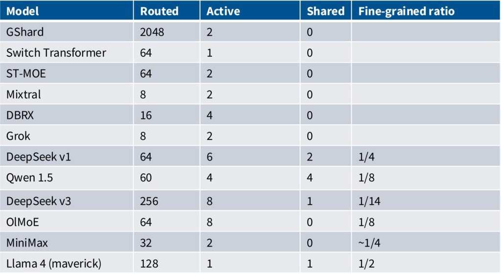
Following DeepSeek’s lead, we see models like Qwen 1.5, DeepSeek V3, and MiniMax—primarily Chinese MoEs—adopting essentially the same approach. While the specific numbers differ, they all use fine-grained experts and often include shared experts, staying very similar to the original DeepSeek MoE configuration.
The ratio column represents how much each expert is sliced relative to a standard dense configuration. For example, DeepSeek with a 1/4 ratio and 64 experts essentially has 16 normally sized stacks, giving them roughly double the FLOPs of a dense equivalent with six routed experts active at any time.
There seems to have been a period where Chinese companies experimented with many shared experts, but people have generally moved back to zero or one shared expert, as the ablations don’t clearly show that even one shared expert is particularly useful.
6. Training Approaches
MoE Training Overview
When it comes to training Mixture of Experts models, we encounter a pretty gnarly challenge.
🔴 The Fundamental Training Dilemma
We cannot afford to turn on all the experts during training because doing so would force us to pay the full computational cost of every expert in the model. Imagine having a model that’s suddenly 256 times more expensive to train—that’s a complete non-starter from a practical standpoint.
This means we absolutely need training-time sparsity to make MoE models feasible.
The Non-Differentiability Problem
This requirement for sparse training creates a significant technical hurdle: sparse gating decisions are inherently non-differentiable. This transforms our training problem into something resembling a reinforcement learning challenge, which is considerably more complex than standard backpropagation.
We’re now dealing with discrete routing decisions that can’t be optimized through traditional gradient-based methods.
Three Approaches to Non-Differentiable Gating
To tackle this non-differentiable gating problem, researchers have developed several approaches:
- Reinforcement Learning: Treating routing decisions as actions in an RL framework
- Bandit-Inspired Methods: Incorporating randomization and exploration to discover effective expert assignments
- Heuristic Solutions: Adding specialized balancing loss terms that encourage more uniform expert utilization
Reinforcement Learning for MoEs
Let’s start by examining the reinforcement learning approach to solving this non-differentiable routing problem.
RL: Principled but Impractical
Reinforcement learning is probably one of the earliest and most principled approaches that people tried for mixture of experts. The logic is straightforward: when you have a non-differentiable routing decision, you can think of that as a policy and throw RL at it to solve the problem.
Unfortunately, while RL via REINFORCE does work, it’s not so much better that it’s a clear win over simpler alternatives.
🔴 Why RL Failed for MoE Routing
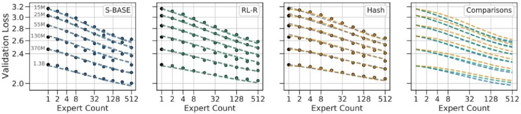
There’s a paper by Clark et al. in 2020 that explored various scaling-related questions in MoEs and included an RL baseline using the REINFORCE baseline approach. But unfortunately, their results show it’s not really that much better than using something as simple as hashing for routing decisions.
What’s particularly interesting is that Clark and colleagues were really focused on benchmarking against something called S-BASE (a linear assignment method), and that approach handily beats doing RL. The fundamental issue is that RL might be the “right solution” in principle, but the gradient variance and complexity means it’s pretty finicky to use in practice.
As far as I know, no one at scale has really used an RL-based approach to optimize these gating decisions.
Stochastic Approximation Methods
Given these limitations with pure RL approaches, what has been done much more at scale is stochastic approximations of various kinds, where you might add perturbations to make the routing differentiable.
Gaussian Noise Perturbations
Here’s an example from Shazeer in 2017, one of the early MoE papers. We start with our original linear affine transformation, which is identical to what we were doing before—basically computing our inputs \(x\) and a learned weight for each gate. But now we jitter it a little bit by adding noise sampled from a normal distribution, and then pick a \(W_{noise}\) scale that’s learned.
$$G(x) = \text{Softmax}(\text{KeepTopK}(H(x), k))$$
$$H(x)_i = (x \cdot W_g)_i + \text{StandardNormal}() \cdot \text{Softplus}((x \cdot W_{noise})_i)$$
$$\text{KeepTopK}(v, k)_i = \begin{cases} v_i & \text{if } v_i \text{ is in the top } k \text{ elements of } v \\ -\infty & \text{otherwise} \end{cases}$$
💡 Exploration-Exploitation Trade-offs
This parameter controls how much noise to inject into the process, and you can think of this as a stochastic exploration policy. By manipulating \(W_{noise}\) in particular ways, like annealing it down, you can control the exploration-exploitation trade-offs.
When you’re adding noise, each expert might randomly get some other tokens that it wasn’t expecting to get, which leads to experts that are less specialized but maybe a bit more robust. The stochasticity also means that you don’t get as much specialization, and that leads to loss of efficiency.
Multiplicative Jitter (Fedus et al. 2022)
There’s another approach where people multiply the router logits with a multiplicative perturbation to get less brittle experts. Stochastic jitter was explored in Fedus et al 2022, which does a uniform multiplicative perturbation for the same goal of getting less brittle experts.
if training:
    # Add noise for exploration across experts
    router_logits += mtf.random_uniform(
        shape=router_logits.shape,
        minval=1-eps,
        maxval=1+eps
    )

# Convert to float32 for stability
router_logits = mtf.to_float32(router_logits)

# Probabilities for each token of what expert it should be sent to
router_probs = mtf.softmax(router_logits, axis=-1)
🔴 Stochastic Routing: Largely Abandoned
However, this jitter process was later removed in Zoph et al 2022 because they found it just didn’t work as well as some of the heuristic loss-based approaches. These stochastic routing tricks were tried in a couple of the early Google papers, but I think that approach has generally been abandoned by most people training these mixture of experts models.
Sections 5-6 Key Takeaways
- Fine-grained experts: Slice experts smaller (1/4 size) to get more experts without parameter cost
- Shared experts: Handle common processing, but benefits are context-dependent
- DeepSeek config: 64 experts, 6 active, 2 shared, 1/4 ratio became the template
- Training challenge: Sparse gating is non-differentiable, requires special techniques
- RL approaches: Principled but impractical—not better than simple hashing
- Stochastic jitter: Explored but largely abandoned in favor of heuristic losses
- Expert collapse: Without balancing, one expert dominates and others die
Part 3: MoE Training Methods and Challenges
Load balancing, expert parallelism, and overcoming training instabilities
7. Load Balancing and Expert Allocation
Heuristic Balancing Losses
Now that we understand the fundamental routing mechanisms in mixture of experts models, we need to address a critical challenge: ensuring tokens are distributed evenly across experts.
The Key Trick: Balancing Losses
Loss balancing is really the key trick to get out of the token allocation problem in mixture of experts models. This is the loss that mostly everyone actually uses to train MoEs, originally introduced in the Switch Transformer from Google in 2022.
$$\text{loss} = \alpha \cdot N \cdot \sum_{i=1}^{N} f_i \cdot P_i$$
$$f_i = \frac{1}{T} \sum_{x \in B} \mathbf{1}\{\arg\max p(x) = i\}$$
$$P_i = \frac{1}{T} \sum_{x \in B} p_i(x)$$
Understanding the Vectors \(f\) and \(P\)
So what are these vectors exactly?
- \(f_i\): For each expert, the fraction of tokens that were actually allocated to expert \(i\). Think of this as a probability vector telling you what fraction of tokens in your batch were routed to expert \(i\).
- \(P_i\): The fraction of router probability that was intended for expert \(i\)—the original softmaxed routing decision.
So \(P_i\) measures the intended probability from the router, while \(f_i\) captures the actual routing decision made by the top-k method.
💡 How the Gradient Works
One interesting aspect is what happens when you take the derivative of that loss with respect to \(p\). Since this is a linear function with respect to \(p_i\), you’ll see that the strongest down-weighting action happens on the experts with the biggest allocations.
It’s actually proportional to the amount of tokens that you get—so you’re going to be pushed downwards more strongly if you’ve got more tokens. This is the basic behavior of this loss, and almost everybody uses this kind of \(f \cdot p\) trick to try to balance tokens across different units.
DeepSeek Balancing Approaches
Building on these foundational balancing concepts, let’s explore how DeepSeek has innovated with more sophisticated approaches.
Per-Expert and Per-Device Balancing
The first approach to balancing in DeepSeek is per-expert balancing per batch, where each batch ensures experts get an even number of tokens. This uses exactly the same \(f \cdot p\) inner product structure as before.
Beyond balancing across experts, you might also want to consider systems concerns since you’re going to shard your experts onto different devices. This leads to another loss with essentially the same structure, but measuring which tokens go to which devices rather than which experts.
$$\mathcal{L}_{\text{ExpBal}} = \alpha_1 \sum_{i=1}^{N’} f_i P_i$$
$$\mathcal{L}_{\text{DevBal}} = \alpha_2 \sum_{i=1}^{D} f_i’ P_i’$$
DeepSeek V3’s Breakthrough: Auxiliary Loss-Free Balancing
DeepSeek V3 actually innovates significantly here—and I don’t think I’ve seen this before. It’s one of the first things in the MoE world that doesn’t actually come from Google. They’ve gotten rid of the expert balancing term entirely and instead take their softmax scores and add a little fudge factor \(B_i\), where \(B_i\) is a per-expert bias score.
$$g’_{i,t} = \begin{cases} s_{i,t}, & s_{i,t} + b_i \in \text{Topk}(\{s_{j,t} + b_j | 1 \leq j \leq N_r\}, K_r), \\ 0, & \text{otherwise}. \end{cases}$$
💡 Online Learning for Expert Biases
Expert \(i\) might get up-weighted or down-weighted—if an expert isn’t getting enough tokens, it gets a higher \(B_i\) allowing it to grab more tokens. They learn \(B_i\) through a simple online gradient scheme:
- Measure at each batch what each expert is getting
- If experts aren’t getting enough tokens → add learning rate \(\gamma\) to \(B_i\)
- If getting too many tokens → subtract \(\gamma\), making that expert slightly less attractive
🔴 Not Fully Auxiliary Loss-Free
They call this auxiliary loss-free balancing, and if you read the DeepSeek V3 paper—which all of you should because it’s really nice—they make a big deal about how this makes training so stable and wonderful.
But then you keep reading the section, and they’re like, “actually, we decided that for each sequence maybe we still want to be balanced, and this doesn’t work well enough, so we’ve added the heuristic loss back!”
So they do have something called the complementary sequence-wise auxiliary loss that is basically exactly the auxiliary loss they decided they needed to balance load at a per-sequence level rather than per-batch level. It’s not fully auxiliary loss-free as they’d like you to believe, but this approach of setting up per-expert bias and using online learning is still quite innovative.
Important Implementation Detail
An important detail is that you only use the \(B_i\) values to make routing decisions—you don’t actually send them over as part of your gating weights.
Regarding whether MoE performance would be better without system optimization concerns: per-expert balancing isn’t really a systems concern. You still want to do this because without it, you’ll find issues with expert utilization. The device-level balancing is more about systems optimization, but the fundamental expert balancing remains important for model performance regardless of hardware considerations.
Impact of Load Balancing Removal
To understand why load balancing is so critical, let’s examine what happens when we remove it entirely.
🔴 Expert Collapse Without Balancing
One of the most compelling pieces of evidence for the importance of load balancing comes from a really nice ablation study that shows exactly what happens when you remove this mechanism.
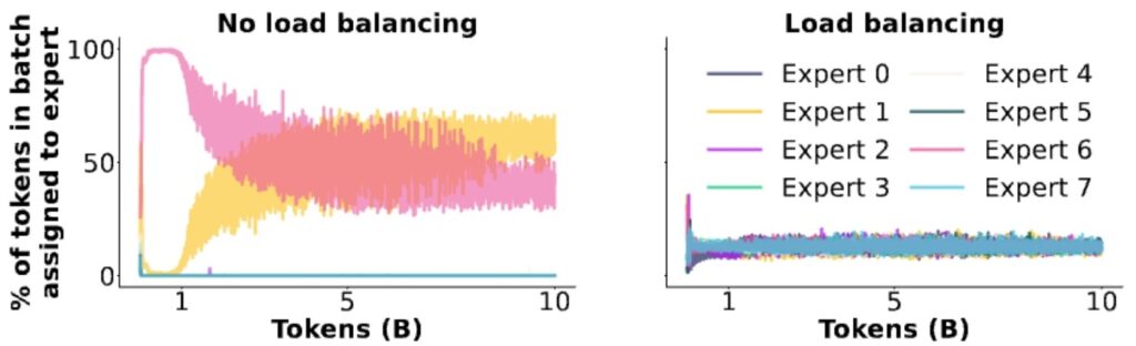
What they find is that early on in training, the model just picks one or two experts, and all the other experts essentially die—the router never sends anything to them. So you’re just wasting memory at that point, and you’ve effectively lost performance for free by getting a smaller model.
Visualizing Expert Death
The ablation results provide a striking visualization of this problem. Looking at the expert assignment patterns, if you don’t implement load balancing, you see that the pink and yellow experts just take over, consuming about 50% of the tokens while all the other experts remain dead and do nothing.
You’ve essentially wasted six out of eight experts and unintentionally created a two-expert mixture of experts model. While this might still be better than a dense model because at least you have two experts working, you could have done much better by properly utilizing all your experts.
8. Training Challenges and Solutions
Systems Complexity and Expert Parallelism
Let’s start by examining the systems challenges that come with implementing Mixture of Experts models.
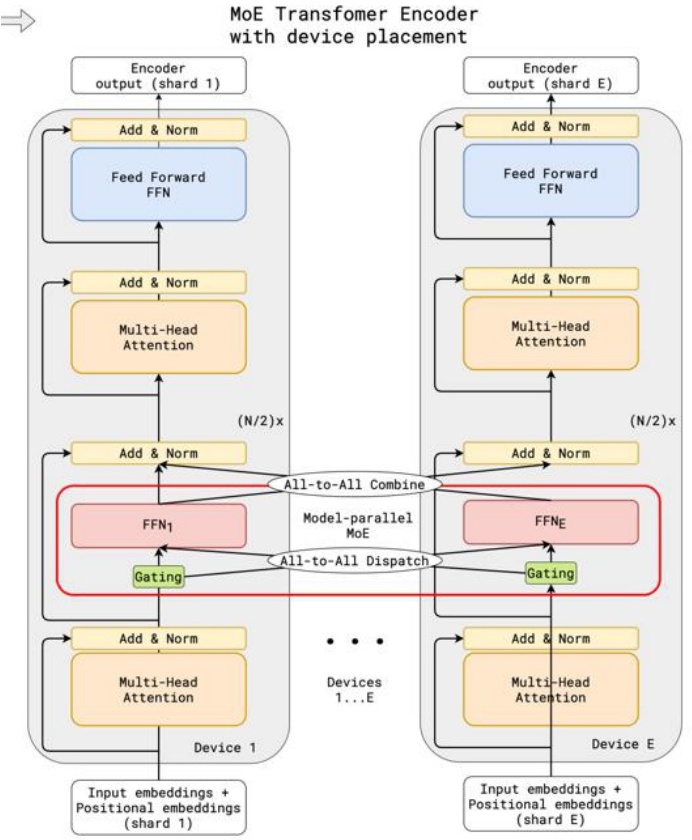
Expert Parallelism: Elegant Distribution
One of the most compelling aspects of MoEs is how elegantly they can be deployed across distributed computing devices. The key concept here is expert parallelism, which involves strategically placing one or just a few experts onto each individual device. This approach creates a natural distribution of computational workload that can scale effectively across multiple processing units.
The Token Processing Workflow
When you’re actually processing a token through this system, the workflow becomes quite interesting:
- Router Decision: First, you hit the router, which makes the crucial decision about which experts should handle this particular token.
- All-to-All Dispatch: After the router picks the relevant experts, you orchestrate a collective communication call (typically all-to-all) that sends tokens to their designated devices.
- FFN Computation: The appropriate feed-forward networks compute their outputs on each device.
- Gather and Combine: Another collective communication call gathers and integrates the results.
💡 Economics of Expert Parallelism
The economics of this approach really depend on whether your feed-forward computations are substantial and “beefy” enough to justify the overhead costs of this expert parallelism communication pattern.
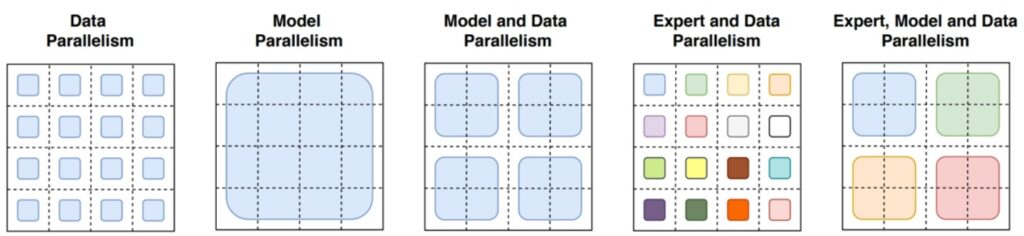
What makes expert parallelism particularly valuable is that it represents another powerful form of parallelism that you can add to your computational toolkit—beyond traditional data or model parallelism approaches.
Model Stochasticity Issues
Building on the complexity of distributed expert systems, there’s actually a fascinating source of randomness inherent in Mixture of Experts that’s worth exploring.
🔴 Token Dropping: A Hidden Source of Randomness
In MoE architectures, tokens get routed to different experts that live on separate devices, and when you’re processing batched queries, these tokens can end up distributed unevenly across experts.
Imagine you have a batch to process with multiple experts available, but for whatever reason, this particular batch really loves expert number three—like all the tokens get routed to expert number three. The problem is that the device hosting expert number three doesn’t have enough memory to handle all those tokens simultaneously.
How Token Dropping Works
This leads to what people call token dropping, which happens at both training and inference time. You often have what’s called a load factor that controls the maximum number of allowed tokens per expert.
When the router allocates too many tokens to a single expert, you simply drop those excess tokens—either for system memory reasons or because you’re worried that expert might dominate during training.
When a token gets dropped: It receives zero computation from the MLP layer and just passes through via the residual connection.
💡 Cross-Batch Effects
This means if your token got dropped, you’ll get a different result than if it hadn’t been dropped, and crucially, this depends on who else is in your batch.
MoEs can thus induce stochasticity at both training and inference time, creating cross-batch effects that you normally never think about during inference. This might explain some mysterious phenomena—like why GPT-4’s API initially gave different responses even with temperature set to zero, which many speculated could be related to non-deterministic routing patterns in MoE models.
Stability and Overfitting Challenges
The stability issues we just discussed become particularly acute in certain training scenarios.
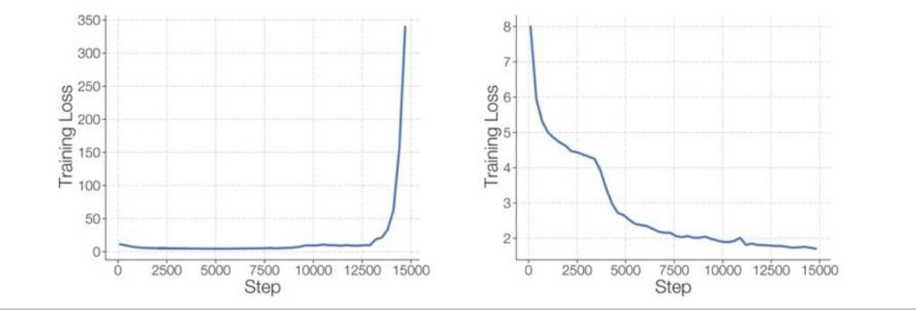
🔴 MoEs Can Blow Up
MoEs have this unfortunate property where they’ll sometimes just blow up on you, particularly when you try to fine-tune them. This instability has been a major concern in the field, with researchers like Barrett and others dedicating entire papers to making MoEs more stable.
The main culprit, as usual, is the softmax function in the router—that’s always where you want to be afraid.
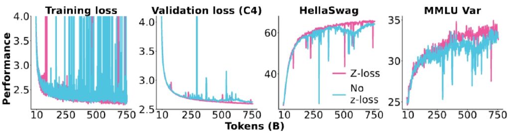
The \(Z\)-Loss Solution
To combat this, practitioners do all router computations in float32 for extra safety, and sometimes add an auxiliary \(Z\)-loss term:
$$L_z(x) = \frac{1}{B} \sum_{i=1}^{B} \left( \log \sum_{j=1}^{N} e^{x_j^{(i)}} \right)^2$$
💡 How \(Z\)-Loss Works
The \(Z\)-loss works by taking the log of the sum of exponentiated values in the softmax, squaring that, and adding it as an extra loss term. This keeps the normalizer values near one, which is excellent for stability.
Interestingly, this is actually one of the earlier applications of \(Z\)-loss before it became more popular for general model training. You can really see the effects in practice—if you remove the \(Z\)-loss from your router function, you’ll observe giant loss spikes in your validation loss where the model goes a bit crazy for a few iterations before getting pulled back.
The Fine-Tuning Overfitting Problem
The overfitting problem becomes particularly pronounced when fine-tuning MoEs on smaller datasets. In the earlier days of MoE research, back in the BERT and T5 era when fine-tuning was the dominant paradigm, researchers observed significant overfitting in sparse models.
You can see this clearly in the large gap between training and validation performance—sparse models show much worse generalization compared to dense models. This makes sense when you consider that you’re fine-tuning these gigantic parameter models on relatively small datasets.
Solutions to Overfitting
Several solutions have emerged to address these overfitting concerns:
- Alternating Architecture: Design MoEs so that not every layer is a MoE layer—alternate between dense layers and MoE layers, then fine-tune only the dense layers
- Massive Data: Simply use massive amounts of data (DeepSeek used 1.4 million training examples)
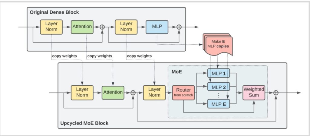
- Upcycling: Start with a pre-trained dense model, copy MLP layers with perturbations, initialize router from scratch, then continue training
Part 3 Key Takeaways
- Balancing loss (\(f \cdot P\)): The key trick—penalize experts that get too many tokens
- DeepSeek V3 innovation: Per-expert bias \(B_i\) with online learning (not fully loss-free though)
- Expert collapse: Without balancing, 1-2 experts dominate and others die
- Expert parallelism: Natural distribution across devices via all-to-all communication
- Token dropping: Creates cross-batch stochasticity at training AND inference
- \(Z\)-loss: Keeps router softmax stable, prevents loss spikes
- Fine-tuning overfitting: Solve with alternating layers, massive data, or upcycling
Continue to Part 4 for Upcycling, DeepSeek Evolution, and Complete Implementation →
Part 4: Advanced MoE Techniques and Case Studies
Upcycling, the complete DeepSeek evolution, and building state-of-the-art MoE systems
9. Model Upcycling Techniques
Dense to MoE Conversion Methods
One of the most cost-effective approaches to creating Mixture of Experts models is through a technique called upcycling, where you initialize the MoE directly from a pre-trained dense model.
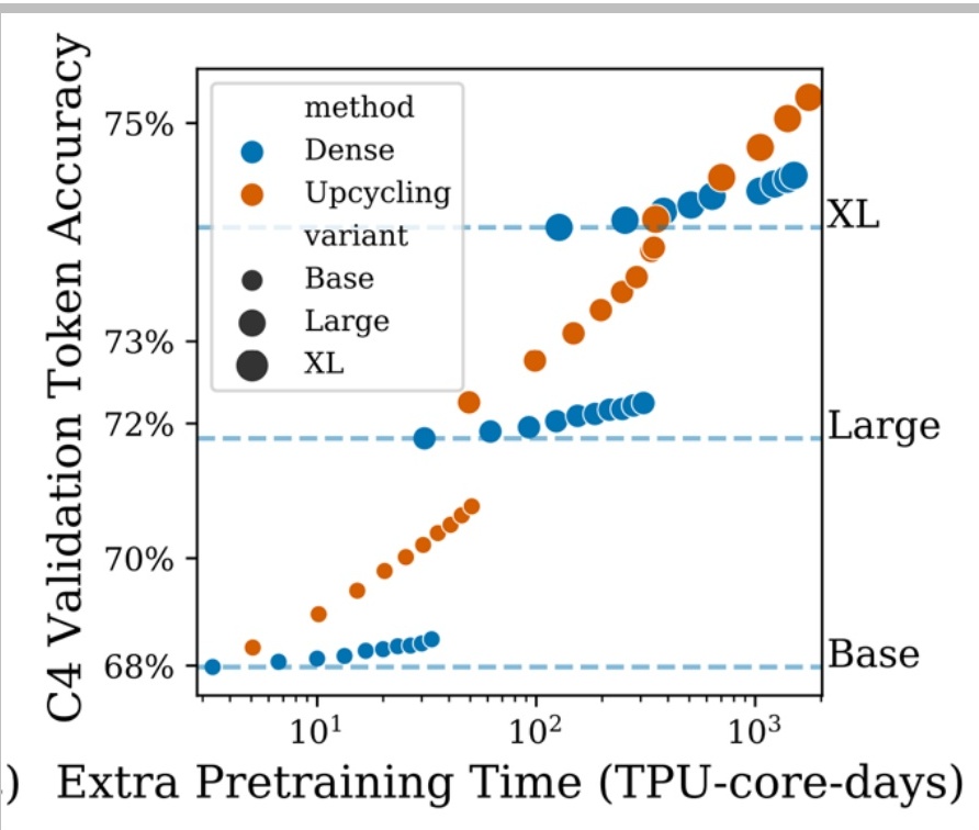
Why Upcycling Matters
This method has proven to be incredibly valuable because it allows you to leverage all the knowledge and representations that have already been learned during the expensive dense training phase. Rather than starting from scratch with a sparse architecture, upcycling provides a smart initialization strategy that can dramatically reduce the computational cost of obtaining a high-quality MoE model.
The Efficiency Advantage
The beauty of MoE models lies in their inference efficiency—not every expert MLP needs to be active during inference time, which means you can effectively get the benefits of a much larger parameter model without actually having to train that massive model from scratch.
This sparse activation pattern is what makes MoE architectures so appealing for scaling up model capacity while keeping computational costs manageable.
MiniCPM Upcycling Example
A great concrete example of successful upcycling comes from MiniCPM, a Chinese open LLM that basically tried to build really good small language models.
💡 MiniCPM’s Configuration
They actually succeeded at taking a dense model and upcycling it into a Mixture of Experts (MoE) architecture. Their approach uses a simple MoE configuration:
- Top-k = 2
- 8 experts
- ~4B active parameters
- ~520B training tokens
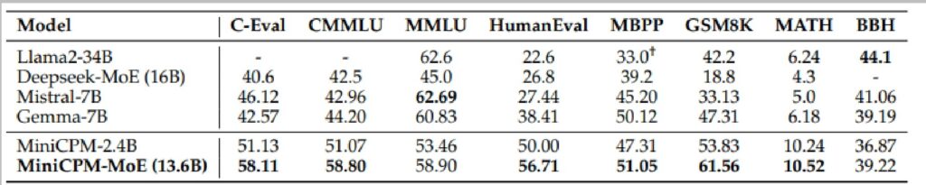
Benchmark Results
Looking at Table 6 with the benchmark results of MiniCPM-MoE, you can see that their numbers get significantly better in the last two rows. Going from the dense model to the MoE, they get a pretty non-trivial bump in performance across multiple evaluation metrics.
The table shows comparisons with other models like Llama2-34B and Qwen1.5-7B, demonstrating the robustness of their improvements.
Qwen MoE Initialization Success
As I mentioned at the start of the lecture, one of Qwen’s earliest and most successful attempts at mixture of experts involved taking one of their existing dense models and building what they called an “upcycled MoE.”
Remarkable Efficiency Gains
This approach yielded fairly significant performance gains, allowing them to achieve models on par with their 7B parameter models using only a 2.7 billion parameter active model—a remarkable efficiency improvement that demonstrates the power of the MoE architecture.
Qwen MoE Configuration
The specific implementation of Qwen MoE was initialized from their Qwen 1.8B model and employed:
- Top-k = 4 routing strategy
- 60 experts total
- 4 shared experts across all tokens
This configuration strikes an interesting balance between computational efficiency and model capacity—by activating only the top 4 most relevant experts for each input, the model maintains a relatively small active parameter count while having access to the specialized knowledge distributed across all 60 experts.
💡 Challenging Traditional Assumptions
What makes this result particularly compelling is how it challenges our traditional understanding of the relationship between model size and performance.
The Qwen team demonstrated that through careful architectural choices and expert specialization, a model with significantly fewer active parameters could match the performance of much larger dense models, opening up new possibilities for efficient large language model deployment and inference.
10. DeepSeek MoE Evolution
DeepSeek Architecture Evolution
To wrap up our exploration of mixture of experts architectures, let’s walk through the DeepSeek MoE evolution and hopefully give you a sense of how modern high-performance open source systems develop.
Understanding DeepSeek V3
I want you to understand the DeepSeek V3 architecture setup and all the changes they made, because it’s an excellent example of iterative improvement. You’ll also appreciate that architectures don’t change that dramatically—DeepSeek V1 basically nailed the core architecture, and subsequent versions refined the details rather than revolutionizing the approach.
DeepSeek MoE V1: The Foundation
The original DeepSeek MoE was a 16 billion parameter model with 2.8 billion active parameters, using:
- 2 shared + 64 fine-grained experts
- 4-6 active at a time
- Standard top-k routing (softmax before top-k selection)
- Auxiliary loss balancing terms at expert and device levels
$$\mathbf{h}_i’ = \mathbf{u}_i + \sum_{j=1}^{N_s} \text{FFN}_j^{(s)}(\mathbf{u}_i) + \sum_{j=1}^{N_r} g_{i,j} \cdot \text{FFN}_j^{(r)}(\mathbf{u}_i)$$
$$g_{i,j} = \begin{cases} s_{i,j}, & s_{i,j} \in \text{Topk}(\{s_{i,l} | 1 \leq l \leq N_r\}, K_r) \\ 0, & \text{otherwise} \end{cases}$$
$$s_{i,j} = \text{Softmax}_j(\mathbf{u}_i^T \mathbf{e}_j)$$
$$\mathcal{L}_{\text{Expert}} = \alpha_1 \sum_{i=1}^{N_r} f_i P_i$$
🔴 DeepSeek V2: Massive Scale + Device-Limited Routing
When DeepSeek moved to V2, they scaled dramatically to 236 billion parameters with 21 billion active, keeping the core architecture identical but adding clever systems optimizations.
The key innovation was addressing the communication cost problem of fine-grained experts. Instead of naively routing to top-K experts across all devices, they introduced a two-stage process:
- First selecting top-M devices with highest affinity scores
- Then performing top-K selection within those M devices
This device-limited routing significantly controls communication costs when scaling to gigantic model sizes.
V2 Communication Balancing Loss
V2 also introduced communication balancing loss to handle both input and output communication costs. For each expert, tokens must be routed in (input communication) and results must be returned to their original devices (output communication).
$$\mathcal{L}_{\text{ComBal}} = \alpha_3 \sum_{i=1}^{D} f_i^{\text{in}} \cdot f_i^{\text{out}}$$
DeepSeek V3: The Current State-of-the-Art
Finally, DeepSeek V3 reached 671 billion parameters with 37 billion active, maintaining the same core MoE architecture but introducing some particularly interesting refinements:
- Normalized gate to one with sigmoid instead of softmax
- Auxiliary loss-free training with dynamic expert bias terms
- Sequence-wise auxiliary loss for inference-time robustness
- Removed communication loss (showing thoughtful design choices)
$$\mathbf{h}_t’ = \mathbf{u}_t + \sum_{i=1}^{N_s} \text{FFN}_i^{(s)}(\mathbf{u}_t) + \sum_{i=1}^{N_r} g_{i,t} \cdot \text{FFN}_i^{(r)}(\mathbf{u}_t)$$
$$g_{i,t}’ = \frac{s_{i,t}}{\sum_{j=1}^{N_r} s_{j,t}}$$
$$s_{i,t} = \text{Sigmoid}(\mathbf{u}_t^T \mathbf{e}_i)$$
DeepSeek V3 Sigmoid Gating
Building on the architectural evolution we just covered, DeepSeek V3 introduces some particularly interesting modifications to their mixture of experts architecture.
From Softmax to Sigmoid
They’ve made a key change by normalizing the gate to one and moving the softmax normalization operation up in the process. However, instead of using exponential gating decisions, they’re actually using sigmoids, which provides a softer and more nicely behaved operation than the traditional softmax approach.
While these changes represent refinements to the system, conceptually this still operates as the same top-K routing decision we’ve seen before.
$$g_{i,t}’ = \begin{cases} s_{i,t}, & s_{i,t} + b_i \in \text{Topk}(\{s_{j,t} + b_j | 1 \leq j \leq N_r\}, K_r), \\ 0, & \text{otherwise}. \end{cases}$$
💡 Thoughtful Design: Adding AND Removing
DeepSeek V3 maintains the top-K improvement from previous versions, which seems like a clever idea worth keeping. However, they haven’t simply added features—they’ve also removed some elements, such as the communication loss.
This shows a thoughtful approach to architecture design where they’re willing to jettison components that may not be providing sufficient value.
11. Complete MoE Implementation
Additional Components for DeepSeek V3
Now that we’ve covered the core MoE architecture, let’s explore some additional innovations that DeepSeek V3 brings to the table.
Multi-Head Latent Attention (MLA)
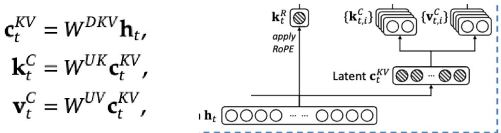
You actually already know all the ingredients needed to understand DeepSeek’s approach to optimizing the KV cache. While we previously discussed GQA and MHA as inference optimizations that reduce the number of heads, the DeepSeek folks take a different approach by projecting the heads into a lower dimensional space.
The Latent Compression Idea
The basic idea is to express the Q, K, V as functions of a lower-dimensional “latent” activation. Instead of generating the Ks and Vs directly from the input hidden states \(h_t\), they first generate a low dimensional compressed version \(c\) that’s smaller and easier to cache.
$$c_t^{KV} = W^{DKV} h_t$$
$$k_t^C = W^{UK} c_t^{KV}, \quad v_t^C = W^{UV} c_t^{KV}$$
$$c_t^Q = W^{DQ} h_t, \quad q_t^C = W^{UQ} c_t^Q$$
💡 The Clever Matrix Merge Trick
The benefits are clear: when KV-caching, we only need to store \(c_t^{KV}\), which can be much smaller than the original high-dimensional \(h_t\).
You might worry about computational overhead from the extra matrix multiply \(W^{UK}\), but here’s the clever part—this matrix can be merged into the Q projection through simple associativity. Since we’re going to compute \(q \cdot k\) in the attention operation anyway, and \(q\) itself has a projection matrix, we can merge \(W^{UK}\) and the Q matrix together into one operation, avoiding any extra computational cost.
🔴 RoPE Conflicts with MLA
However, there’s a subtle complexity: RoPE conflicts with MLA-style caching. The issue is that RoPE rotation matrices \(R_q\) and \(R_k\) get in between the query projection and the latent vector up-projection matrix, preventing us from reordering the matrix multiplies.
Their solution is to have a few non-latent key dimensions that can be rotated, working around this incompatibility while maintaining the benefits of the compressed representation.
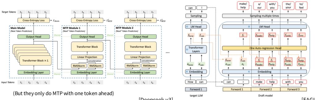
Multi-Token Prediction (MTP)
The final innovation is Multi-Token Prediction (MTP), a minor change to their loss function where they predict multiple tokens in parallel.
Normally, you shift inputs left by one to predict the next token, but with MTP, they take the hidden state and pass it through a very lightweight one-layer transformer that can predict further into the future. This allows the model to predict not just the next token, but tokens multiple steps ahead.
$$h_t^k = M_k[\text{RMSNorm}(h_t^{k-1}); \text{RMSNorm}(\text{Emb}(t_{t+k}))]$$
$$h_{1:T-k}^k = \text{TRM}_k(h_{1:T-k}^{k-1})$$
$$P_{t+k+1}^k = \text{OutHead}(h_t^k)$$
💡 MTP in Practice
However, somewhat disappointingly, they only implement MTP with one token ahead, despite having diagrams showing how it could work for many tokens. Still, these technical innovations showcase the sophisticated engineering that goes into modern MoE systems.
MoE Summary and Key Concepts
As we wrap up our deep dive into MoE architectures, it’s worth reflecting on why Mixture of Experts have now emerged as a cornerstone technology for building and deploying high-performance, large-scale systems.
The Fundamental Insight: Sparsity
The fundamental insight behind MoEs is their ability to leverage sparsity—the recognition that you don’t need all parameters active all the time, and not all inputs require the full computational power of the entire model.
This sparse activation pattern allows MoEs to scale efficiently while maintaining performance, making them particularly attractive for resource-constrained environments.
The Primary Challenge: Discrete Routing
The primary technical challenge in MoEs lies in discrete routing, which is arguably one of the main reasons why MoEs didn’t immediately gain widespread adoption when first introduced.
The prospect of having to optimize discrete top-k routing decisions can be quite daunting from an optimization perspective. However, what’s remarkable is that heuristic approaches to this routing problem somehow seem to work effectively in practice, despite the theoretical complexities involved.
💡 The Bottom Line
Today, there’s substantial empirical evidence demonstrating that MoEs are not just theoretically sound but practically effective, especially in FLOP-constrained settings.
The accumulated research and real-world deployments have shown that MoEs represent a cost-effective approach to scaling neural networks. This combination of theoretical elegance and practical utility has positioned MoEs as a fundamental architecture choice for modern large-scale machine learning systems.
🎯 Complete Guide Key Takeaways
- MoE = Sparse FFN activation: Same FLOPs, more parameters, better performance
- Top-K routing dominates: \(K=2\) most common, token choice over expert choice
- Fine-grained experts: Slice experts smaller (1/4 size) for more experts without parameter cost
- Balancing loss is essential: Without it, experts collapse to 1-2 dominant ones
- DeepSeek innovations: Per-expert bias, sigmoid gating, device-limited routing
- \(Z\)-loss for stability: Keeps router softmax from exploding
- Upcycling works: Convert dense models to MoE for efficiency gains
- MLA for KV cache: Compress to latent space, merge matrices cleverly
- Expert parallelism: Natural distribution across devices via all-to-all communication
- Heuristics work: Despite non-differentiable routing, practical solutions succeed
The Evolution Summary
| Model | Total Params | Active Params | Key Innovation |
|---|---|---|---|
| DeepSeek V1 | 16B | 2.8B | Fine-grained + Shared experts |
| DeepSeek V2 | 236B | 21B | Device-limited routing |
| DeepSeek V3 | 671B | 37B | Sigmoid gating + MLA + MTP |
Thank You for Reading!
This guide covered the complete landscape of Mixture of Experts architectures—from fundamentals to state-of-the-art implementations. MoE has evolved from a research curiosity to the dominant architecture powering the world’s most capable AI systems. Whether you’re building your own models or understanding frontier AI, these concepts are now essential knowledge.
Resources: DeepSeek V3 Paper • Fedus et al. 2022 Survey • Olmo MoE Paper • Switch Transformer
These lecture notes are designed according to Lecutre 4- Large Language Models from Scratch 2025 – Stanford University – YouTube.