LLMs from Scratch #002 PyTorch Fundamentals: Building Efficient Language Models from Scratch

PyTorch Fundamentals: Building Efficient Language Models from Scratch
🎯 What You’ll Learn
In this comprehensive guide, we’ll explore the fundamental building blocks of PyTorch for language model development. You’ll learn how to account for memory usage across different floating-point representations, understand tensor operations and their computational costs, master efficient data movement between CPU and GPU, and develop the mindset of resource accounting that’s essential for training large-scale models. This is the practical foundation you need before diving into transformer architectures.
Tutorial Overview
- Memory Accounting: Understanding Tensors and Data Types
- Floating Point Representations: From FP32 to BF16
- Compute Fundamentals: Moving Between CPU and GPU
- Tensor Operations: Views, Strides, and Memory Efficiency
- Matrix Multiplications and Batched Operations
- Einops: Named Dimensions for Better Code
- Computational Cost: Counting FLOPs
1. Why Efficiency Matters: A Napkin Math Exercise
Before we dive into the technical details, let’s motivate why understanding resource accounting is crucial. Here’s a real-world question: how long would it take to train a 70 billion parameter dense transformer model on 15 trillion tokens using 1,024 H100 GPUs?
Example 1: Training Time Calculation
Question: How long would it take to train a 70B parameter model on 15T tokens on 1024 H100s?
# Step 1: Calculate total FLOPs needed
total_flops = 6 * 70e9 * 15e12

# Step 2: Determine hardware specs
h100_flop_per_sec = 1979e12 / 2  # Theoretical peak / 2
mfu = 0.5  # Model FLOPs Utilization

# Step 3: Calculate FLOPs available per day
flops_per_day = h100_flop_per_sec * mfu * 1024 * 60 * 60 * 24

# Step 4: Divide to get training time
days = total_flops / flops_per_day
# Result: ~144 days
The factor of 6 comes from the computational cost of both forward and backward passes through the model. The H100 has a theoretical peak of 1979 teraFLOP/s (divided by 2 for the precision we’re using), but we assume an Model Flops Utilization – MFU of 0.5—real-world efficiency is typically around 50% of theoretical peak.
💡 Example 2: Maximum Model Size
Question: What’s the largest model you can train on 8 H100s using AdamW (naively)?
# Step 1: Calculate available memory
h100_bytes = 80e9  # 80GB per H100

# Step 2: Account for memory per parameter
# 4 bytes: parameters
# 4 bytes: gradients
# 8 bytes: optimizer state (AdamW stores two momentum terms)
bytes_per_parameter = 4 + 4 + (4 + 4)

# Step 3: Calculate maximum parameters
num_parameters = (h100_bytes * 8) / bytes_per_parameter
# Result: ~40 billion parameters
Caveat: This rough calculation doesn’t account for activations, which depend on batch size and sequence length and can consume significant memory.
📝 Note: This is a rough back-of-the-envelope calculation. These estimates help you get in the right ballpark before investing significant time and resources. As you’ll learn throughout this guide, the devil is in the details—but having these rough numbers in your head is invaluable for quick sanity checks.
🔴 The Efficiency Imperative
When these numbers get large, they directly translate into dollars. To be efficient in deep learning, you need to know exactly how many FLOPs you’re expending, how much memory you’re consuming, and where your bottlenecks are. This isn’t just academic knowledge—it’s the difference between a successful training run and burning through your compute budget with nothing to show for it.
The rest of this guide will teach you the mechanics and mindset needed to perform these calculations and optimize your models accordingly.
2. Memory Accounting: Understanding Tensors
Tensors are the fundamental building blocks in deep learning. They store everything: parameters, gradients, optimizer states, data, and activations. Understanding their memory footprint is the first step toward efficient model development. We have wrote a complete series on PyTorch so in case that you need to refresh your knowledge, have a look here. There are Deep Learning, both theoretical and practical hands on examples.
💡 Creating Tensors: Multiple Approaches
PyTorch provides several ways to create tensors depending on your needs:
import torch

# From existing data
x = torch.tensor([[1., 2, 3], [4, 5, 6]])

# Matrix of zeros
x = torch.zeros(4, 8)  # 4x8 matrix of all zeros

# Matrix of ones
x = torch.ones(4, 8)  # 4x8 matrix of all ones

# Random normal distribution
x = torch.randn(4, 8)  # 4x8 matrix of iid Normal(0, 1) samples

# Uninitialized memory
x = torch.empty(4, 8)  # 4x8 matrix of uninitialized values
Use empty() when you want to allocate memory but plan to fill it with custom initialization logic later:
import torch.nn as nn

# Custom initialization with truncated normal
x = torch.empty(4, 8)
nn.init.trunc_normal_(x, mean=0, std=1, a=-2, b=2)
For more details: Check the PyTorch documentation on tensors for a comprehensive reference.
The Basic Memory Formula
Memory usage for a tensor is remarkably simple:
Memory = Number of Elements × Size of Each Element
For example, a 4×8 matrix with float32 values contains 32 elements. Each float32 takes 4 bytes (32 bits ÷ 8). Therefore, the total memory usage is 32 × 4 = 128 bytes.
To put this in perspective, consider a single matrix from the feed-forward layer of GPT-3. With dimensions of approximately 12,288 × 49,152, using float32 representation, that’s one matrix consuming 2.3 gigabytes of memory. These matrices can get big fast.
Floating Point 32: The Default Standard
Float32, also known as FP32 or single precision, is the gold standard in computing and the default in PyTorch.
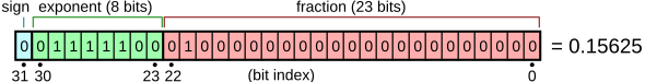
It uses 32 bits allocated as follows:
- 1 bit for sign
- 8 bits for exponent (providing dynamic range)
- 23 bits for fraction (providing resolution)
💡 Precision vs. Full Precision
You might hear float32 referred to as “full precision,” but this is context-dependent. If you’re talking to scientific computing researchers, they’ll point out they use float64 or higher. But in machine learning, float32 is generally the maximum you need—deep learning is “sloppy” in that sense, and the extra precision often doesn’t improve model performance.
3. Beyond Float32: Optimizing Memory with Lower Precision
Given that tensors can consume gigabytes of memory, and we’re working with models containing billions of parameters, there’s a natural desire to use less memory. The solution: lower-precision floating-point representations.
Float16: The Half-Precision Trade-off
Float16 Structure
Float16 (FP16 or half precision) uses only 16 bits, cutting memory usage in half:
- 1 bit for sign
- 5 bits for exponent (reduced from 8)
- 10 bits for fraction (reduced from 23)
The problem? Dynamic range suffers significantly. If you try to create a tensor with a value like 1e-8 in float16, it rounds to zero—you get underflow:
import torch

# Demonstrating underflow in float16
x_fp32 = torch.tensor([1e-8], dtype=torch.float32)
x_fp16 = torch.tensor([1e-8], dtype=torch.float16)

print(f"FP32: {x_fp32.item()}")  # Output: 1e-08
print(f"FP16: {x_fp16.item()}")  # Output: 0.0 (underflow!)
Float16 struggles with both very small and very large numbers, which can cause instability during training, especially for large models with many matrices.
BF16: The Deep Learning Solution
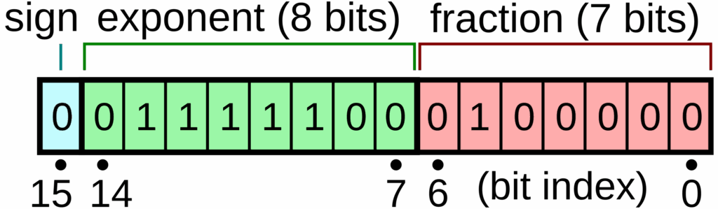
Brain Float 16 (BF16)
Developed in 2018, BF16 was specifically designed to address deep learning’s needs. The key insight: dynamic range matters more than resolution for neural networks.
Why BF16 Works Better
BF16 allocates its 16 bits differently than FP16:
- More bits for exponent: Same 8 bits as FP32
- Fewer bits for fraction: Only 7 bits instead of FP32’s 23
The result: BF16 uses the same memory as FP16 but maintains the dynamic range of FP32. The trade-off is worse resolution, but this doesn’t matter much for deep learning applications.
When you create a tensor with 1e-8 in BF16, you actually get a non-zero value—no more underflow issues:
import torch

# BF16 maintains dynamic range
x_fp32 = torch.tensor([1e-8], dtype=torch.float32)
x_bf16 = torch.tensor([1e-8], dtype=torch.bfloat16)

print(f"FP32: {x_fp32.item()}")   # Output: 1e-08
print(f"BF16: {x_bf16.item()}")   # Output: ~1e-08 (non-zero!)
FP8: Pushing the Limits Further
In 2022, Nvidia introduced FP8, using just 8 bits to represent floating-point numbers. With so few bits available, it’s quite crude, and there are two variants depending on whether you prioritize resolution or dynamic range. FP8 is only supported on H100 GPUs and later generations, making it less universally available.
💡 Practical Precision Guidelines
Float32: Safe default, higher memory usage, good for parameters and optimizer states
BF16: Typically used for computations during training—cast your parameters to BF16, run the forward pass, but maintain float32 for things that accumulate over time
Float16: Generally not recommended for deep learning anymore
FP8: Cutting edge, limited hardware support
Mixed Precision Training
You can become more sophisticated by analyzing your training pipeline and determining the minimum precision needed at each stage. For example, some practitioners use float32 for attention mechanisms to prevent instability while using BF16 for simple feed-forward matrix multiplications and gradient accumulation.
import torch

# Example: Mixed precision training pattern
params = torch.randn(1024, 1024, dtype=torch.float32)

# Cast to BF16 for forward pass computation
params_bf16 = params.to(dtype=torch.bfloat16)

# Run computations with BF16
output = some_computation(params_bf16)

# But keep optimizer states in float32 for accumulation
optimizer_state = torch.zeros_like(params)  # Stays in float32
🔴 The Accumulation Principle
Critical insight: Parameters and optimizer states need float32 because they’re accumulated over time. You can think of BF16 as something transitory—you cast your parameters to BF16, run your forward pass with that model, but the values you’re updating incrementally over thousands of iterations need higher precision.
4. Compute Fundamentals: CPU vs. GPU
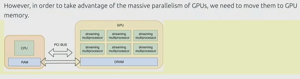
Understanding where your tensors live is just as important as understanding their size and precision. By default, PyTorch creates tensors on the CPU, which is a problem—if you’re not using your GPU, you’ll be orders of magnitude slower.
The Hardware Architecture
Your system has a CPU with its own RAM and a GPU with separate high-bandwidth memory (HBM). For example, an H100 GPU has 80 gigabytes of HBM. Moving data between CPU RAM and GPU memory requires explicit data transfer operations that take time.
The mental model: Always keep in your mind where each tensor resides. Just looking at a variable or code snippet won’t tell you—you need to track it explicitly. Consider using assertions in your code to document and verify tensor locations.
Moving Tensors to GPU
PyTorch provides straightforward methods for moving tensors and creating them directly on the GPU:
💡 Tensor Movement Patterns
import torch

# By default, tensors are on CPU
x = torch.randn(32, 32)
print(x.device)  # Output: cpu

# Method 1: Move existing tensor to GPU
x = x.to('cuda')
print(x.device)  # Output: cuda:0

# Method 2: Create directly on GPU
y = torch.randn(32, 32, device='cuda')
print(y.device)  # Output: cuda:0
Verification: Check memory allocation before and after tensor creation. For a 32×32 matrix of float32 values, you should see exactly 4,096 bytes (32 × 32 × 4) allocated:
import torch

# Check GPU memory allocation
memory_before = torch.cuda.memory_allocated()

# Create tensor on GPU
x = torch.randn(32, 32, device='cuda')

memory_after = torch.cuda.memory_allocated()
memory_used = memory_after - memory_before

print(f"Memory used: {memory_used} bytes")
# Expected: 4096 bytes (32 * 32 * 4)
🔴 The Data Transfer Problem
Critical point: Data movement between CPU and GPU is expensive. Whenever you have a tensor, you should always keep in your mind where it resides. Just looking at the variable or code won’t tell you—you need to track it explicitly. Consider using assertions in your code to document and verify tensor locations:
import torch

def forward(x, weight):
    # Document and verify tensor locations
    assert x.device.type == 'cuda', "Input must be on GPU"
    assert weight.device.type == 'cuda', "Weight must be on GPU"

    return x @ weight
Understanding Tensor Storage: Under the Hood
So what exactly is a tensor in PyTorch? Tensors are mathematical objects, but in PyTorch’s implementation, they’re actually pointers into allocated memory with metadata that describes how to access any element of the tensor.
5. Under the Hood: How Tensors Really Work
Tensors aren’t just mathematical objects—in PyTorch, they’re pointers into allocated memory with metadata that specifies how to index into that storage.
The Storage and Stride System
When you create a 4×4 matrix, PyTorch actually stores it as a long one-dimensional array. The tensor maintains metadata called “strides” that specify how to convert multi-dimensional indices into positions in that array.
For a 2D tensor, you have two strides:
- Stride 0: How many elements to skip when moving to the next row (e.g., 4 for a 4-column matrix)
- Stride 1: How many elements to skip when moving to the next column (typically 1)
To access element [1, 2], you calculate: position = 1 × stride[0] + 2 × stride[1] = 1 × 4 + 2 × 1 = 6

Views: Multiple Tensors, One Storage
This storage system enables a powerful feature: multiple tensors can share the same underlying storage with different views. This means you can create different ways of looking at the same data without copying it.
import torch

# Create a 2x3 matrix
x = torch.tensor([[1., 2, 3], [4, 5, 6]])
print("Original x:")
print(x)
# Output:
# tensor([[1., 2., 3.],
#         [4., 5., 6.]])

# Get row 0 - creates a view
y = x[0]  # @inspect y
assert torch.equal(y, torch.tensor([1., 2, 3]))
assert torch.equal(x.untyped_storage(), y.untyped_storage())  # Same storage!

# Get column 1 - creates a view
y = x[:, 1]  # @inspect y
assert torch.equal(y, torch.tensor([2, 5]))
assert torch.equal(x.untyped_storage(), y.untyped_storage())  # Same storage!

# View 3x2 matrix as 2x3 matrix - creates a view
x_reshaped = torch.tensor([[1., 2], [3, 4], [5, 6]])
y = x_reshaped.view(2, 3)  # @inspect y
assert torch.equal(y, torch.tensor([[1, 2, 3], [4, 5, 6]]))
assert torch.equal(x_reshaped.untyped_storage(), y.untyped_storage())  # Same storage!
💡 Common View Operations
Slicing rows: y = x[0] creates a view of the first row
Slicing columns: y = x[:, 1] creates a view of column 1
Transposing: y = x.transpose(1, 0) creates a transposed view
Reshaping: y = x.view(3, 2) reinterprets dimensions
Key point: None of these operations copy data. They all share the same underlying storage.
The Transpose Operation
import torch

x = torch.tensor([[1., 2, 3], [4, 5, 6]])

# Transpose the matrix
y = x.transpose(1, 0)  # @inspect y
print("Transposed y:")
print(y)
# Output:
# tensor([[1., 4.],
#         [2., 5.],
#         [3., 6.]])

assert torch.equal(y, torch.tensor([[1, 4], [2, 5], [3, 6]]))
assert torch.equal(x.untyped_storage(), y.untyped_storage())  # Same storage!
🔴 The Mutation Hazard
Critical warning: If you start mutating one tensor that shares storage with another, both tensors will be affected since they’re just different pointers into the same memory.
import torch

x = torch.tensor([[1., 2, 3], [4, 5, 6]])
y = x[0]  # View of first row

# Mutating x also mutates y!
x[0][0] = 100  # @inspect x, @inspect y
assert y[0][0] == 100  # y changed too!

print(f"x[0][0] = {x[0][0]}")  # 100
print(f"y[0] = {y[0]}")        # 100
This can lead to subtle bugs if you’re not careful about tracking which tensors share storage.
Contiguous vs. Non-Contiguous Tensors
Some views are “contiguous“—if you iterate through the tensor, you’re just walking through the underlying array in order. But some views, like transposed matrices, are non-contiguous. When you transpose, you’re now jumping around in memory as you traverse the logical tensor.
import torch

x = torch.tensor([[1., 2, 3], [4, 5, 6]])
y = x.transpose(1, 0)  # @inspect y

# Check if tensor is contiguous
assert not y.is_contiguous()

# Trying to view non-contiguous tensor will fail
try:
    y.view(2, 3)
    assert False  # Should not reach here
except RuntimeError as e:
    assert "view size is not compatible with input tensor's size and stride" in str(e)

# Solution: make it contiguous first
y_contiguous = x.transpose(1, 0).contiguous().view(2, 3)  # @inspect y_contiguous
assert not torch.equal(x.untyped_storage(), y_contiguous.untyped_storage())  # Different storage now!
Best Practices for Views
Views are free—they don’t allocate memory. Feel free to use them liberally to make your code more readable by defining different variables for different perspectives on your data.
However, remember that .contiguous() and .reshape() (which calls contiguous internally if needed) can create copies, so use them judiciously when memory is tight.
Key takeaway: Views are free, copying takes both (additional) memory and compute.
Element-wise Operations
These operations apply some function to each element of the tensor and return a new tensor of the same shape:
import torch

x = torch.tensor([1., 4, 9])

# Power operation
assert torch.equal(x.pow(2), torch.tensor([1, 16, 81]))

# Square root
assert torch.equal(x.sqrt(), torch.tensor([1, 2, 3]))

# Reciprocal square root (rsqrt): 1/sqrt(x_i)
assert torch.equal(x.rsqrt(), torch.tensor([1, 1/2, 1/3]))

# Addition (element-wise)
assert torch.equal(x + x, torch.tensor([2, 8, 18]))

# Multiplication (element-wise)
assert torch.equal(x * 2, torch.tensor([2, 8, 18]))

# Division (element-wise)
assert torch.equal(x / 0.5, torch.tensor([2, 8, 18]))
Triangular Matrices for Causal Attention
The triu() function takes the upper triangular part of a matrix, which is particularly useful for computing causal attention masks in transformers:
import torch

# Create a 3x3 matrix of ones
x = torch.ones(3, 3).triu()  # @inspect x

assert torch.equal(x, torch.tensor([
    [1, 1, 1],
    [0, 1, 1],
    [0, 0, 1]
]))
💡 Causal Attention Masks
This is useful for computing a causal attention mask, where M[i, j] is the contribution of token i to token j. In causal (autoregressive) language models, token i can only attend to tokens at positions ≤ i, which is exactly what the upper triangular pattern enforces.
6. Matrix Multiplications and Batched Operations
Matrix multiplication is the bread and butter of deep learning. While a basic matrix multiplication takes a 16×32 matrix times a 32×2 matrix to produce a 16×2 result, real machine learning applications operate on batches.
Basic Matrix Multiplication
import torch

# Basic matrix multiplication
x = torch.ones(16, 32)
W = torch.ones(32, 2)
y = x @ W

assert y.size() == torch.Size([16, 2])
Batched Operations
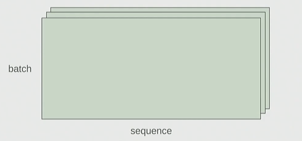
In language models, you typically process multiple examples simultaneously, and each example contains multiple tokens. Your tensors have dimensions like:
- Batch: Number of examples being processed together
- Sequence: Number of tokens in each example
- Hidden: Feature dimension for each token
The Batched Pattern
PyTorch handles batched matrix multiplications elegantly. When you multiply a 4D tensor with a 2D weight matrix, it automatically performs the matrix multiplication for every position in the batch and sequence dimensions.
import torch

# Batched matrix multiplication
# Shape: [batch, sequence, input_dim, hidden_dim]
x = torch.ones(4, 8, 16, 32)

# Weight matrix: [hidden_dim, output_dim]
W = torch.ones(32, 2)

# Matrix multiply across last dimension
y = x @ W

# Result: [batch, sequence, input_dim, output_dim]
assert y.size() == torch.Size([4, 8, 16, 2])
In this case, PyTorch iterates over the first 2 dimensions of x (batch and sequence) and performs the matrix multiplication W for each position, producing an output tensor with shape [4, 8, 16, 2].
🔴 The Dimension Tracking Problem
Traditional PyTorch code is hard to read:
import torch

# Traditional PyTorch code
x = torch.ones(2, 2, 3)  # batch, sequence, hidden
y = torch.ones(2, 2, 3)  # batch, sequence, hidden
z = x @ y.transpose(-2, -1)  # batch, sequence, sequence

# Easy to mess up the dimensions (what is -2, -1?)...
Is -2 the sequence dimension or the hidden dimension? You have to mentally track this, which becomes error-prone as code complexity grows.
Better Dimension Tracking with Jaxtyping
How do you keep track of tensor dimensions? One approach is to use type hints with jaxtyping to document dimension names:
💡 Jaxtyping for Documentation
from jaxtyping import Float
import torch

# Old way (no dimension names)
x = torch.ones(2, 2, 1, 3)  # batch seq heads hidden

# New (jaxtyping) way - dimensions are documented
x: Float[torch.Tensor, "batch seq heads hidden"] = torch.ones(2, 2, 1, 3)
Note: This is just documentation (no enforcement). The type annotation doesn’t actually verify the shapes at runtime, but it makes your code much more readable and self-documenting.
Understanding FLOPs and Computational Cost
Now that we can write clearer code with einops, let’s examine the computational cost of our operations. Understanding FLOPs (floating-point operations) is essential for reasoning about model training time and hardware requirements.
What is a FLOP?
Two Confusing Acronyms (Pronounced the Same!)
- FLOPs: floating-point operations (measure of computation done)
- FLOP/s: floating-point operations per second (also written as FLOPS), which is used to measure the speed of hardware
A floating-point operation (FLOP) is a basic operation like addition (x + y) or multiplication (x × y).
Hardware Performance: A100 and H100
💡 GPU Performance Numbers
# Peak performance specs
a100_flop_per_sec = 312e12  # 312 teraFLOP/s

# H100 with sparsity: 1979 teraFLOP/s
# H100 without sparsity: approximately 50%
h100_flop_per_sec = 1979e12 / 2  # ~990 teraFLOP/s in practice
Important note about sparsity: The asterisk (*) on H100 specs means “with sparsity”. This refers to a specific structured sparsity pattern where 2 out of 4 elements in each group of 4 must be zero. In practice, nobody uses this because it requires very specific model architectures. As the lecturer notes: “The marketing department uses it.”
🔴 Precision Matters
The FLOP/s you can achieve depends heavily on numerical precision:
- FP32 (32-bit floats): Really bad performance on modern GPUs – orders of magnitude slower
- FP16 (16-bit floats): Much better, the standard for training
- FP8 (8-bit floats): Even faster if you’re willing to accept lower precision
Modern deep learning almost never uses FP32 for training. If you’re running FP32 on an H100, you’re wasting money.
Intuitions: How Big Are These Numbers?
To calibrate your intuition about FLOPs:
- Training GPT-3 (2020): 3.14e23 FLOPs
- Training GPT-4 (2023): Speculated to take 2e25 FLOPs
- US Executive Order (now revoked in 2025): Any foundation model trained with ≥ 1e26 FLOPs must be reported to the government
Back-of-the-Envelope Calculations
Let’s do a simple calculation: how many FLOPs can we get from 8 H100s running for 2 weeks?
import torch

# 8 H100s for 2 weeks
# 60 and 60 : seconds and minutes
# 24 and 7 : hours and weeks
total_flops = 8 * (60 * 60 * 24 * 7) * h100_flop_per_sec  # @inspect total_flops
# Result: approximately 4.7e21 FLOPs
You can use these kinds of back-of-the-envelope calculations to estimate training time or compare computational budgets across different models.
Example: FLOPs for a Linear Model
Let’s work through a concrete example. Even a simple linear model gives us the building blocks for understanding more complex architectures.
import torch

# Setup
if torch.cuda.is_available():
    B = 16384   # Number of points
    D = 32768   # Dimension
    K = 8192    # Number of outputs
else:
    B = 1024
    D = 256
    K = 64

device = torch.device('cuda' if torch.cuda.is_available() else 'cpu')
x = torch.ones(B, D, device=device)  # Data matrix
w = torch.randn(D, K, device=device)  # Weight matrix
y = x @ w  # Linear model output
Question: How many FLOPs was that?
The Matrix Multiplication FLOP Formula
When you perform matrix multiplication, for every (i, j, k) triple, you:
- Multiply two numbers together (one multiplication)
- Add that result to an accumulator (one addition)
Therefore, the total FLOPs is:
# For matrix multiplication: x (B×D) @ w (D×K) = y (B×K)
actual_num_flops = 2 * B * D * K  # @inspect actual_num_flops
Formula to remember: For matrix multiplication, FLOPs = 2 × (product of all three dimensions)
That’s 2 × (left dimension) × (middle dimension) × (right dimension).
FLOPs of Other Operations
The FLOPs of other operations are usually linear in the size of the tensor:
- Element-wise operation on m×n matrix: O(m·n) FLOPs
- Addition of two m×n matrices: m·n FLOPs
💡 Key Insight
In general, no other operation you encounter in deep learning is as expensive as matrix multiplication for large enough matrices.
This is why most “napkin math” for deep learning models focuses exclusively on counting the matrix multiplications that the model performs. For large models, the cost of other operations (activations, layer norms, etc.) becomes negligible compared to the matrix multiplications.
When Other Operations Matter
Of course, there are regimes where your matrices are small enough that the cost of other operations starts to dominate. But generally, for the kinds of large-scale models we’re discussing, matrix multiplication is the bottleneck.
Interpretation
Understanding FLOPs gives you several useful capabilities:
- B is the number of data points: More data points = more compute
- (D·K) is the number of parameters: More parameters = more compute
- Training time estimation: If you know the FLOPs and your hardware’s FLOP/s, you can estimate training time
- Hardware budgeting: You can contextualize FLOP counts with model costs to plan computational budgets
9. Computing Gradients: The Backward Pass
When training neural networks, we need to understand not just the forward pass computation, but also the cost of computing gradients. Let’s explore how gradient computation affects our overall training budget.
Simple Linear Model Example
Consider a simple linear model where we take predictions and compute the Mean Squared Error (MSE) loss with respect to a target value of 5. While this isn’t a particularly interesting loss function, it’s illustrative for understanding gradient computation.
In the forward pass, you have your input x and weights w (which we want to compute gradients for). You make a prediction using a linear product, then calculate your loss. In the backward pass, you simply call loss.backward(), and the gradient—stored as a variable attached to the tensor—gives you exactly what you need.
Most people have computed gradients in PyTorch before, but let’s dig deeper into how many FLOPs are required for this operation.
Two-Layer Linear Network Analysis
Let’s examine a more complex scenario: a two-layer linear model. The architecture consists of:
- Input
xwith shape (b, d) - First weight matrix
w1with shape (d, d) - Hidden activations
h1 - Second weight matrix
w2transforming to k dimensions - Final output and loss computation
💡 Forward Pass FLOPs
For the forward pass, we need to:
import torch

# First layer: x @ w1 -> h1
h1 = x @ w1  # Requires 2 * b * d * d FLOPs

# Second layer: h1 @ w2 -> h2
h2 = h1 @ w2  # Requires 2 * b * d * k FLOPs
The total forward FLOPs equals two times the product of all dimensions in each matrix multiplication. In other words, it’s approximately two times the total number of parameters in this case.
Backward Pass Complexity
The backward pass is more involved. We need to compute gradients with respect to multiple variables: h1, h2, w1, and w2.
Chain Rule for Gradient Computation
For w2, we apply the chain rule. The gradient with respect to w2 involves computing the gradient of the loss with respect to h2, then multiplying by h1:
import torch

# Gradient with respect to w2 using chain rule
# w2_grad = h1.T @ (loss_grad_h2)
w2_grad = torch.sum(h1 * loss_grad_h2, dim=0)
This gradient computation essentially looks like a matrix multiplication, so the same FLOP calculation applies: 2 × b × d × k.
However, this is only the gradient for w2. We also need to compute the gradient with respect to h1 to continue backpropagating to w1 and beyond.
🔴 Critical Insight: Backward Pass Cost
The backward pass requires approximately the same computational cost as the forward pass, if not more. For each parameter gradient we compute, we’re essentially performing operations similar to forward pass matrix multiplications. This means training (forward + backward) roughly doubles or triples your computational requirements compared to inference alone.
10. Parameter Initialization: Avoiding Training Instability
Proper parameter initialization is crucial for stable training. Let’s explore why naive initialization can cause problems and how to fix it.
The Problem with Naive Initialization
Consider initializing a weight matrix W (input_dim × hidden_dim) using a standard normal distribution:
import torch

# Naive initialization - seems innocuous
W = torch.randn(input_dim, hidden_dim)
output = input @ W
When you feed input through this layer, the output values grow as approximately the square root of the hidden dimension. For large models, this causes outputs to explode, making training very unstable.
💡 Xavier/Glorot Initialization
The solution is to rescale by the square root of the number of inputs:
import torch

# Proper initialization
W = torch.randn(input_dim, hidden_dim) / (input_dim ** 0.5)

# Now outputs remain stable
output = input @ W  # Values concentrate around Normal(0, 1)
This approach ensures that the output distribution remains stable regardless of model size. It’s known as Xavier initialization (or Glorot initialization, up to a constant) and has been extensively explored in deep learning literature.
Extra Safety: Truncated Normal
For additional stability, you might want to avoid the unbounded tails of the normal distribution. A common practice is to truncate values outside the range [-3, 3]:
import torch

# Truncated normal initialization
W = torch.randn(input_dim, hidden_dim) / (input_dim ** 0.5)

# Don't trust normal because it has unbounded tails
# Truncate to [-3, 3] to avoid large values
W = torch.clamp(W, -3, 3)
This prevents any extreme values from entering your network and potentially destabilizing training.
11. Building a Custom Model in PyTorch
Let’s put our knowledge into practice by building a simple deep linear network.
The “Cruncher” Model
We’ll create a custom model with multiple linear layers, each performing matrix multiplication without activation functions. It’s going to have d dimensions and multiple layers:
import torch
import torch.nn as nn

class Cruncher(nn.Module):
    def __init__(self, d, n_layers):
        super().__init__()
        # Create n_layers of d×d matrices
        self.layers = nn.ModuleList([
            nn.Linear(d, d) for _ in range(n_layers)
        ])
        # Final output layer
        self.head = nn.Linear(d, 1)

    def forward(self, x):
        # Pass through all layers
        for layer in self.layers:
            x = layer(x)
        # Apply final head
        return self.head(x)
The total number of parameters is: d² + d² + d = 2d² + d (for a 2-layer version with a 1-dimensional output).
💡 Using the Model
import torch

# Initialize model
d = 512
model = Cruncher(d=d, n_layers=2)

# Check parameter count
num_params = sum(p.numel() for p in model.parameters())
# Result: d² + d² + d = 2d² + d

# Move to GPU for faster computation
model = model.cuda()

# Generate random data and run forward pass
x = torch.randn(32, d).cuda()  # batch_size=32
output = model(x)

print(f"Output shape: {output.shape}")  # [32, 1]
12. Randomness and Reproducibility
Randomness appears in many places during neural network training, and managing it properly is essential for debugging and reproducibility.
🔴 Why Randomness Matters
Randomness shows up everywhere:
- Parameter initialization
- Dropout layers
- Data ordering and shuffling
- Data augmentation
When trying to reproduce a bug or compare different approaches, uncontrolled randomness can make it impossible to isolate what’s causing different behavior. Randomness can be annoying in some cases if you’re trying to reproduce a bug, for example.
Best Practice: Fixed Random Seeds
Always set fixed random seeds for reproducibility, and ideally use a different random seed for every source of randomness:
import torch
import numpy as np
import random

# Set all random seeds
torch.manual_seed(42)
np.random.seed(42)
random.seed(42)

# For CUDA operations
torch.cuda.manual_seed(42)
torch.cuda.manual_seed_all(42)  # For multi-GPU
Pro tip: Having a different random seed for every source of randomness is nice because then you can, for example, fix initialization or fix the data ordering, but vary other things. This gives you fine-grained control during debugging.
Determinism is your friend when you’re debugging. The ability to reproduce exact behavior makes it much easier to track down issues and verify fixes.
💡 Multiple Sources of Randomness
In code, there are many places where you can use randomness. Just be cognizant of which one you’re using. If you want to be safe, just set the seed for all of them:
- PyTorch’s random number generator
- NumPy’s random number generator
- Python’s built-in random module
- CUDA’s random number generator
13. Efficient Data Loading
For large-scale training, efficient data loading is critical. Language models often work with massive datasets that won’t fit in memory.
Memory-Mapped Files
In language modeling, data is typically a sequence of integers (output from a tokenizer) serialized into NumPy arrays. For massive datasets like Llama’s 2.8 terabytes of training data, you can’t load everything into memory at once.
The solution is np.memmap, which creates a memory-mapped file. You can sort of pretend to load it by using this handy function, which gives you essentially a variable that is mapped to a file:
import numpy as np

# Memory-mapped array - doesn't load entire file
data = np.memmap('huge_dataset.npy', dtype=np.int32, mode='r')

# When you try to access the data, it actually on-demand loads the file
batch = data[1000:1032]  # Only loads this slice
This gives you a variable that behaves like a NumPy array but is actually mapped to a file. When you access the data, it loads on-demand from disk, allowing you to work with datasets far larger than your available RAM.
Using that, you can create a data loader that samples data from your batch.
14. Optimizers: The Engine of Training
With our model defined, we need an optimizer to update parameters. Let’s explore the evolution of optimization algorithms.
Optimizer Family Tree
1. Stochastic Gradient Descent (SGD)
The simplest approach: compute the gradient on your batch and take a step in that direction, no questions asked.
2. Momentum
Dating back to classic optimization work by Nesterov, momentum maintains a running average of gradients and updates against this average instead of the instantaneous gradient. This helps smooth out noisy gradients.
3. Adagrad
Scales gradients by the average of squared past gradients. You scale the gradients by the average over the norms of your—or actually not the norms, but the square of the gradients. This gives different learning rates to different parameters based on their history.
4. RMSprop
An improved version of Adagrad that uses an exponential moving average rather than a flat average of squared gradients, preventing the learning rate from becoming too small.
5. Adam (2014)
The current standard, combining RMSprop and momentum. It maintains both a running average of gradients and a running average of squared gradients.
15. Implementing Custom Optimizers
Understanding how to implement optimizers helps demystify what’s happening during training. Let’s implement Adagrad from scratch.
💡 Adagrad Implementation
import torch
from torch.optim import Optimizer

class Adagrad(Optimizer):
    def __init__(self, params, lr=0.01, eps=1e-10):
        defaults = dict(lr=lr, eps=eps)
        super().__init__(params, defaults)

    def step(self):
        for group in self.param_groups:
            for p in group['params']:
                if p.grad is None:
                    continue

                # Access optimizer state for this parameter
                state = self.state[p]

                # Initialize sum of squared gradients if needed
                if 'sum_of_squares' not in state:
                    state['sum_of_squares'] = torch.zeros_like(p.data)

                # Get current gradient (assumed already calculated)
                grad = p.grad.data

                # Update sum of squared gradients (element-wise)
                state['sum_of_squares'] += grad ** 2

                # Put it back into the state
                g2 = state['sum_of_squares']

                # Update parameters
                # Divide by square root of accumulated squared gradients
                p.data -= group['lr'] * grad / (torch.sqrt(g2) + group['eps'])
How It Works
Parameter Groups: Parameters are organized by groups (e.g., layer0, layer1, final weights). Your parameters are grouped by, for example, you have one for the layer zero, layer one, and then the final weights.
State Dictionary: You can access a state dictionary that maps from parameters to whatever optimizer state you want to store (like sum of squared gradients for Adagrad).
Gradient Assumption: The gradient for each parameter is assumed to be already calculated by the backward pass before optimizer.step() is called.
Element-wise Operations: The squaring of gradients is an element-wise squaring of the gradient, and you put it back into the state. The division by the adaptive learning rate is also element-wise, meaning each parameter gets its own adaptive learning rate based on its history.
💡 Using the Custom Optimizer
import torch

# Create model and optimizer
model = Cruncher(d=512, n_layers=2).cuda()
optimizer = Adagrad(model.parameters(), lr=0.01)

# Define some data
x = torch.randn(32, 512).cuda()
y = torch.randn(32, 1).cuda()

# Forward pass
output = model(x)
loss = ((output - y) ** 2).mean()

# Compute gradients (backward pass)
loss.backward()

# Optimizer updates parameters
# This is where the optimizer actually becomes active
optimizer.step()

# Don't forget to zero gradients for next iteration!
optimizer.zero_grad()
These notes are based on Lecture 2 of Stanford’s CS336 (Spring 2025) by Tatsunori Hashimoto. Large Language Models from Scratch. Stanford, YouTube.
Key Takeaways
- Gradient Computation Cost: The backward pass requires approximately the same computational resources as the forward pass, effectively doubling or tripling your training FLOPs compared to inference.
- Initialization Matters: Use Xavier/Glorot initialization (dividing by √input_dim) to prevent activation magnitudes from exploding as models grow larger.
- Reproducibility is Essential: Always set random seeds for all sources of randomness. Determinism is your friend when debugging.
- Efficient Data Loading: Use memory-mapped files for large datasets that don’t fit in RAM, allowing on-demand loading.
- Optimizer Evolution: Modern optimizers like Adam combine momentum with adaptive learning rates, maintaining both running averages of gradients and squared gradients.
- State Management: Custom optimizers maintain state dictionaries to track optimizer-specific information (like sum of squared gradients) for each parameter.
With these practical PyTorch techniques, you’re equipped to build efficient, reproducible training pipelines for your deep learning projects!