#005 TF 2.0 An implementation of a Shallow Neural Network with tf.keras – Circles dataset
Highlights: In previous post we have talked about TensorFlow Wrappers and there we concluded that tf.keras is the most convenient way to build neural networks. Now we are going to implement one very simple network using this high-level API.
Tutorial Overview:
1. Imports and Dataset preparation
Let’s start with basic imports. Don’t worry if some things are not familiar with all of these libraries, we will use them only for some advanced visualization at the end.
The problem we will tackle within this post will be the classification of points in the Circle dataset. There are two ways to make such points, either by hand or using pre-existing functions from sklearn library. In order to create this artificial dataset we will show both ways.
After our dataset is created, we can visualize and check the shapes of our data. By scattering both classes and both train and test sets, we can see the graphical representation and how hard our problem will be to solve.
By looking at our graphical representation, we can see that the classes are clearly distinguished with not that much noise present.
2. Building a Neural Network
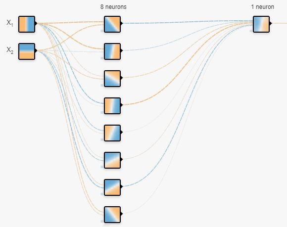
Now it is time to start using TensorFlow 2.0 in order to build our neural network. We will skip the theory part now. In case you need a refresher about neural nets, see here. The easiest way to do this is by using the Sequential API. The practice is to wrap it all up in some function, which we will also do here. After this, to create a network, we will just call that function. The good start for this problem will be the network with \(1\) hidden layer with \(8\) neurons and one output layer. The input data has two features, \(x\) and \(y\), so the input to this network will have the shape of \(2\). In Keras, the input layer itself is not a layer, but a tensor. It is the starting tensor we will send to the first hidden layer.

In tf.keras, Sequential model represents the linear stack of layers where in Dense layers all neurons between layers are connected with each other.
Here, we will use Adam optimizer. Nowadays, it is practically a default optimization algorithm which is used to train neural nets.
To make this work in Keras we need to compile a model. An important choice to make is the loss function. We use the binary_crossentropy loss because we have only two classes.
After training, we can use our model to make predictions. Evaluating the model on training and test sets will give us both loss and accuracy values.
3. Visualization
Let’s now visualize the outputs of our neural network. We can also see the exact value of weights and biases that our network learn over time. This can be done by using get_weights() function.
Now we can visualize the output of each neuron. This can be done by calculating the output by the following equation.

First we need to define our own activation functions for this. We will do this in order to visualize how our network decides how to do the classification.
Let us compute the output of each neuron in our network, step by step.
We can simplify the previous equations by using the vectorization principle.
Now we can visualize the output of each neurons.
A 3D representation can sometimes be very interesting. There we can see transition region where it is not clearly in which class points will be sorted.
If we want to rotate this, we can make use of the Plotly library.
In the next post we will learn how to perform classification using a shallow neural network on Moons dataset using tf.keras.