CamCal 006 Ideal vs Real Intrinsic Parameters
Highlights: Here, we are going to talk about intrinsic camera calibration. We will present the main difference between ideal and real intrinsic parameters, how to improve them, and how to combine them. Here we will also talk about camera parameters, which will be of great importance for further understanding.
Tutorial Overview:
- Intro
- Ideal vs Real Intrinsic Parameters
- Improving Intrinsic Parameters
- Combining Extrinsic and Intrinsic Calibration Parameters
- Other Ways
- Camera Parameters
1. Intro
So first, just to remind. As we said before, there are two parts of geometric calibration in general. The first transformation is from some arbitrary world coordinate system, to the camera system or the camera pose, and these was the extrinsic parameters. They mapped from world coordinates to camera coordinates.
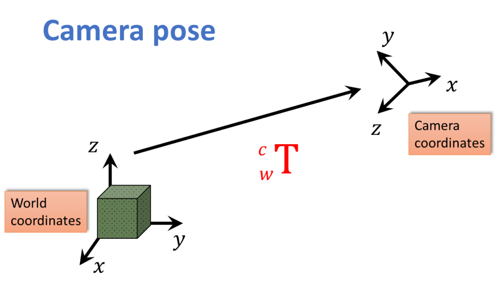
When we write it as \(_{W}^{C}\textrm{T} \) it takes you from the world, to the camera.
We expressed it in terms of homogeneous coordinates, where we had a world coordinate \(\overrightarrow{_{ }^{W}\textrm{p}} \), and it was homogeneous so there is a \(1 \) down there.
$$ \begin{bmatrix}\mid \\\overrightarrow{_{ }^{C}\textrm{p}}\\\mid \\\mid\end{bmatrix}=\begin{bmatrix}- & – & -\\ -& _{W}^{C}\textrm{R} &- \\ – & – &- \\ 0 & 0 & 0\end{bmatrix}\begin{bmatrix}\mid \\\overrightarrow{_{W}^{C}\textrm{t}}\\\mid \\ 1\end{bmatrix}\begin{bmatrix}\mid \\ \overrightarrow{_{ }^{W}\textrm{p}}\\ \mid \\ 1\end{bmatrix} $$
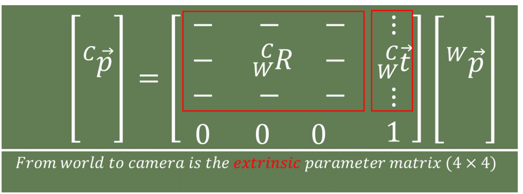
And we combine it with both the rotation component and the translation component to get the three dimensional point in camera coordinates.
So, that world to camera matrix referred to as the extrinsic parameters or the extrinsic parameter matrix. We also said that, that encodes six degrees of freedom, three translation, three rotation.
Here, we are going to talk about the second transformation which goes from the 3D camera coordinates to the 2D image coordinates or the 2D image plane. And these are referred to as the intrinsic parameters, and we will again come up with the intrinsic parameter matrix.
2. Ideal vs Real Intrinsic Parameters
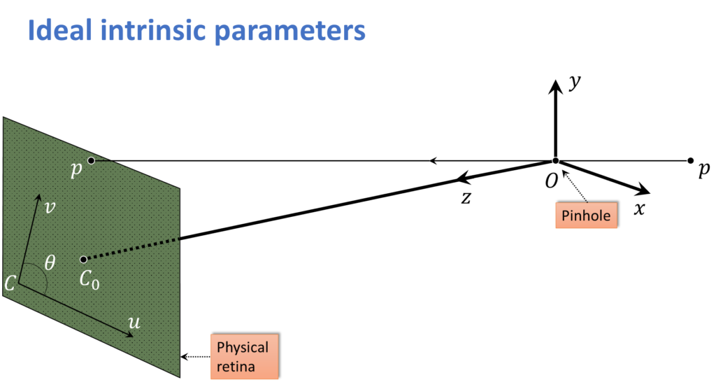
If you have read our previous posts, you might say, didn’t we already do this? We did the ideal perspective projection, where we said that some value \(u \) was just going to be the focal length times \(x \) divided by \(z \), and \(v \) was \(y \) divided by \(z \) multiplied by \(f \), as well.
$$ u = f\frac{x}{z} $$
$$ v = f\frac{y}{z} $$
So you might ask, aren’t we done? Well, no, because that would be in some idealized world. The first problem going back to here is, \(f \) might be in millimeters, so we might have a 10 millimeter lens, or a 50 millimeter lens, but the screen pixels, they are in some arbitrary coordinate. That depends upon exactly how many pixels we get per millimeter in the sensor.
Scale factors \(\alpha\) and \(\beta \)
So the first thing we need to do is to introduce an \(\alpha\) that is just going to scale that value, because we don’t really know what \(f \) is. Now sometimes people will give you \(f \), a focal length, in pixels, which is kind of a weird thing. But what they’re actually doing is, they are giving you this combined value that is sort of the conversion from millimeters to pixels times millimeters, just given to you in pixels. But basically, because they may be in some arbitrary units, we have a scale factor \(\alpha \). So that’s one degree of freedom.
But, who said the pixels are square? Now, it turns out pixels are more
And so now we are introducing \(\beta \). So now we have two degrees of freedom. But we are not done.
Offset
Next, well you remember we put the center of projection, when we were doing the ideal projection. We put the center of projection tight at the camera coordinates system. As if the image was taken so that \(\left ( 0,0 \right ) \) was right in the middle. But of course, we don’t have any guarantee of this. The image may have been cropped out of a section of the window. Or the location of the image actual sensor might not be lined up with the optical axis of the camera. So we have two offsets, \(u_{0} \) and \(v_{0} \) and now we are up to four degrees of freedom. Two scale factors and two offsets.
$$ u = \alpha \frac{x}{z} + u_{0} $$
$$ v = \beta \frac{y}{z} + v_{0} $$
And there is more. We are assuming that the \(u \) direction and the \(v \) direction are actually perpendicular. What if there is actually a little bit of a skew? So that is what is shown in this figure here.
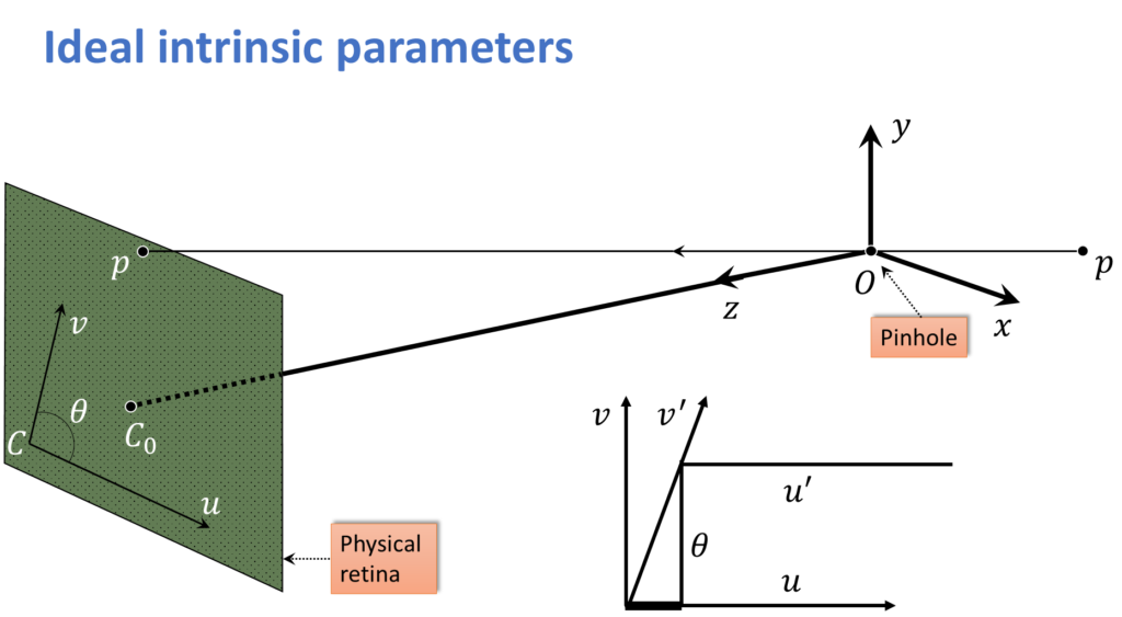
$$ {v}’sin(\theta) = v $$
$$ {u}’ = u – cos(\theta ){v}’ = u – cot(\theta )v $$
The idea is that the actual sampling of \(u \), \(v \) are not perpendicular, and they are off by some angle \(\theta\). So that is what these equations are showing you here. They are showing you the relationship between the \({v}’ \)which is measured and the actual \(v\) , the \({u}’ \)and the actual \(u \).
$$ u = \alpha \frac{x}{z} – \alpha cot(\theta )\frac{y}{z} + u_{0} $$
$$ v = \frac{\beta }{sin(\theta )}\frac{y}{z} + v_{0} $$
So this is the intrinsic parameter representation. And now we have an \(\alpha \) and \(\beta \), the two scale factors. That is two degrees of freedom. \(u_{0}\) and \(v_{0} \) for the two offsets. Plus \(\theta \) which is the skew.
3. Improving Intrinsic Parameters
This is pretty ugly, and we need to make it nicer, and we are going to do that through two ways.
$$ u= \alpha \frac{x}{z}-\alpha cot\left ( \theta \right )\frac{y}{z}+u_{0} $$
$$ v= \frac{\beta }{sin\left ( \theta \right )}\frac{y}{z}+v_{0}$$
First here we have those equations and the first thing you will notice is that we are dividing the \(x \) and the \(y \) with \(z \). And so that should tell us that intrinsic parameters in non-homogeneous coordinates. Next, we are going to move to homogeneous coordinates by putting this whole thing in a matrix formulation.
$$ \begin{bmatrix}z\times u\\z\times v\\z\end{bmatrix}= \begin{bmatrix}\alpha & -\alpha cot\left ( \theta\right ) & u_{0} & 0 \\ 0& \frac{\beta }{sin\left ( \theta \right )} & v_{0} & 0 \\ 0 & 0 & 1 & 0\end{bmatrix}\begin{bmatrix}x\\y\\z\\1\end{bmatrix} $$
So now we can express the whole thing in homogeneous coordinates. Notice that here we have $$\begin{bmatrix}z\times u\\z\times v\\z\end{bmatrix} $$ so later when we convert back from homogeneous to non-homogeneous, we divide by \(z \), and we get what we want. We have the \(\begin{bmatrix}x\\y\\z\\1\end{bmatrix} \) over here, and we have this matrix in the middle. So we can rewrite this as very simple equation where we have a three-dimensional point in the camera frames.
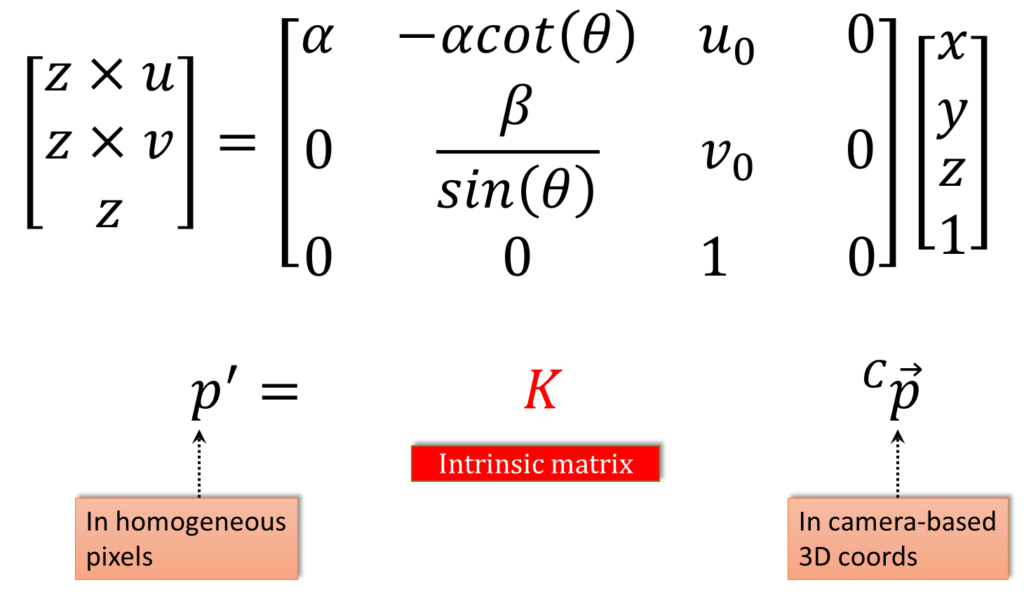
So remember, we have gone from some arbitrary world frame to the three-dimensional camera frame. And we go from that to the homogeneous pixel representation, like that, in the image. So the matrix that takes them from the camera to the image, that is the intrinsic matrix. Hence that matrix represents the intrinsic parameters. Now fortunately, we can make it look even nicer than this. The first thing to notice is that the last column of \(K \), when we write \(K \) as a \(3\times 4 \) matrix, the last column of \(K \) is zeros. And that doesn’t really do very much, so we can get rid of it. And then we can do even more.
Here we have our kinder, gentler intrinsics.
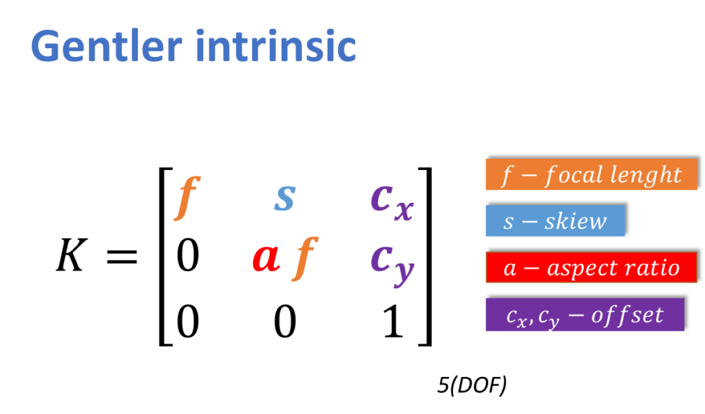
Or even simpler. We are going to remove that last column. And we have gotten rid of the explicit \(\theta\). We have \(f\), which is focal length, \(a \), which is aspect ratio, \(s\), which is for skew, and \(c_{x}\) and \(c_{y}\), are the offsets. Also, remember we said we can have two different scales. A scale for \(u \) and a scale for \(v\). Or what we can have is a focal length and a relative scale between the two. Normally, we tend to think of it that way, as a focal length. That is the overall focal length of the image. And then, if there is a non-uniform relationship between the width and the height, we include that as an aspect ratio. And we are up to five degrees of freedom.
Now, it turns out, this can get even easier. And the way it gets really easy is we assume, if we have square pixels, if there is no skew, and if the optical center is actually in the middle.
$$ K= \begin{bmatrix}f & 0 & 0\\ 0 & 0 & f\\0 & 0 &1\end{bmatrix} $$
Then we have no \(a \), we have no \(s \), we have no \(c_{x} \) and no \(c_{y} \). All we have left is \(f \) which is the only degree of freedom left. So when we are doing a calibration, sort of a lightweight calibration, what we will do is we will just search for \(f \), assuming that our optical axis is in the middle, assuming there is no skew, and assuming that our pixels are square.
4. Combining Extrinsic and Intrinsic Calibration Parameters
So now we found the intrinsic matrix, and also earlier we found the extrinsic matrix. Now we can combine them to get the total camera calibration that goes from a world point all the way through the camera coordinate to the image. So we write down our two equations here. We have our intrinsic:
$$ \overrightarrow{{p}’}= K\overrightarrow{_{ }^{C}\textrm{p}} $$
And our extrinsic:
$$ \begin{bmatrix}\mid \\\overrightarrow{_{ }^{C}\textrm{p}}\\\mid \\\mid\end{bmatrix}=\begin{bmatrix}- & – & -\\ -& _{W}^{C}\textrm{R} &- \\ – & – &- \\ 0 & 0 & 0\end{bmatrix}\begin{bmatrix}\mid \\\overrightarrow{_{W}^{C}\textrm{t}}\\\mid \\ 1\end{bmatrix}\begin{bmatrix}\mid \\ \overrightarrow{_{ }^{W}\textrm{p}}\\ \mid \\ 1\end{bmatrix} $$
This equation relates the world point, to the camera point. \(\overrightarrow{_{ }^{W}\textrm{p}} \) is the world three dimensional coordinates transformed by the extrinsic matrix, becomes the camera three dimensional coordinates, which is used also in the intrinsic equation. Then that is converted to pixels directly.

One thing to note here, is that our world coordinate system, is a four vector, it is a homogeneous. And we get out of four vector, but as we said before, for our \(K\), instead of using the \(3\times 4 \), we can use the \(3\times 3\), in which case we just use the \(\begin{bmatrix}x\\ y\\ z\end{bmatrix}\) of the point in the 3D camera space. We don’t have to use the whole $$ \begin{bmatrix}x\\ y\\ z\\ 1\end{bmatrix} $$ That is basically saying that this \(K\) can be thought of as a \(3\times 4\), or a \(3\times 3\). And when it is a \(3\times 3\), we don’t have to have that \(1\) on the bottom there.
So, putting these two equations together, what we have is we take a world point, we combine it with our extrinsic.
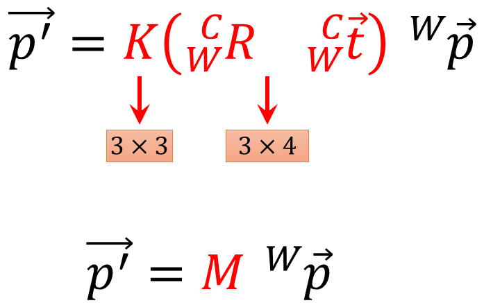
$$ \overrightarrow{{p}’}= K\left ( _{W}^{C}\textrm{R}\times \overrightarrow{_{W}^{C}\textrm{t}} \right ) \overrightarrow{_{ }^{W}\textrm{p}} $$
$$ \overrightarrow{{p}’}= M\times\overrightarrow{_{ }^{W}\textrm{p}} $$
So, this is a \(3\times 4 \) matrix which gets us out of three dimensional vector. And then we combine that with our intrinsic matrix, and that get us our homogeneous image coordinates. So this is a three vector. This whole thing can be written as a single matrix \(M \).
5. Other Ways to Write the Same Equation
Now we just need to write that, \(M \) in a slightly different way, because it is the way that we are actually going to make use of when we solve for this thing.
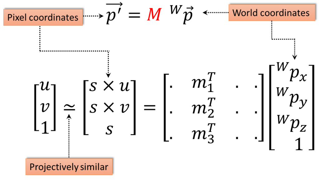
$$ \begin{bmatrix}u\\v\\1\end{bmatrix}\simeq \begin{bmatrix}s\times u\\ s\times v\\s\end{bmatrix}= \begin{bmatrix}. &m _{1}^{T} &. & .\\. & m _{2}^{T} & . & .\\. &m_{3}^{T} &. & .\end{bmatrix}\begin{bmatrix}_{ }^{W}\textrm{p}_{x}\\_{ }^{W}\textrm{p}_{y}\\ _{ }^{W}\textrm{p}_{z}\\ 1\end{bmatrix} $$
So, here we have the same equations written out. You see, we have the world coordinates mapped through \(M \), gives us the homogenous pixel coordinates. And what we have done, we have taken this \(M \) matrix, which, remember, is a \(3\times 4 \)and we have also introduced something new here. We are using \(s \) as a scale, instead of \(z \), and so we have \(s\times u \), \(s\times v\) and \(s\).
To get out \(u \) and \(v \), we just divide by \(s \). And we have put this little operator \(\simeq \) and it is what is known as projectively similar. So you will notice that this vector before and this vector after the operator are exactly the same except for a scale factor. The vector on the left multiplied by \(s \), gives you the vector on the right. And remember, in homogeneous coordinates or using the projective, those two vectors are essentially the same, because when we use their values, we divide out by the left, by the last, component. So, that is what is referred to as projectively similar, so that is also introduced here.
$$ u= \frac{m_{1}\times \overrightarrow{P}}{m_{3}\times \overrightarrow{P}} $$
$$ v= \frac{m_{2}\times \overrightarrow{P}}{m_{3}\times \overrightarrow{P}} $$
The way we recover \(u \) and \(v \) is, we divide the dot product, the dot of the vector of the point \(p \) in the world with the first row, divided by that dot product with the third row, that is what is right here. And then to get the \(v \) value, we do the same thing, but now with the second row.
So basically, what we have to find when we are going to do camera calibration, is, we have to find those \(m \) elements.
6. Camera Parameters
So finally, we can talk about full camera parameters or camera and calibration matrix. The camera and its matrix \(M \), and sometimes it is called \(\Pi \), as we know, is described by several parameters:
- Translation \(T \) of the optical center from the origin of world coordinates.
- Rotation \(R \) of the coordinate system.
- Focal length and aspect, (\(f \), \(a \)). Pixels or pixel size \(\left ( s_{x},s_{y} \right ) \). A principle point, that is the offset \(\left ( {x}’_{c},{y}’_{c} \right ) \). And skew \( \left ( s \right ) \).
- And in this slide, the blue parameters are called the extrinsics and the red are the intrinsics.
$$ x\simeq \begin{bmatrix}sx\\sz\\s\end{bmatrix}= \begin{bmatrix}\ast & \ast & \ast & \ast \\ \ast & \ast & \ast &\ast \\ \ast & \ast & \ast &\ast\end{bmatrix}\begin{bmatrix}X\\ Y\\Z\\1\end{bmatrix}= MX $$
And we can put the whole thing together, we want to find this as a sort of a single matrix. \(M \) is going to be built up of all of the effects of our parameters, and so that looks like this.

$$ M= \begin{bmatrix}f & s &{x}’_{c} \\ 0 & af &{y}’_{c} \\0 & 0 & 1\end{bmatrix}\begin{bmatrix}1 & 0 & 0 &0 \\0 & 1 &0 & 0\\ 0& 0 & 1 &0\end{bmatrix}\begin{bmatrix}R_{3\times 3} & 0_{3\times 1}\\0_{1\times 3} & 1\end{bmatrix}\begin{bmatrix}I_{3\times 3} & T_{3\times 1}\\0_{1\times 3}&1\end{bmatrix}$$
What this says is that \(M\) is a combination of translation, this is extrinsic, and rotation. So now we have the point in the 3D camera coordinate system. Project, this is just the extraction of the \(x \), \(y \), and \(z \), and then we combine that with the intrinsics. And we are up to 11 degrees of freedom. Five for the intrinsics, three for the rotation, three for the translation. That equation there, that \(M \), that is the full camera calibration matrix.
Summary:
Altogether we have covered all the things which we will need for camera calibration in practice. In the next post, we are going to talk more about code and we will show in practice how this works.